SU(4) spin-orbit critical state in one dimension

Abstract

Effect of quantum fluctuations concerned with the orbital degrees of freedom is discussed for the model with SU(4) symmetry in one dimension. An effective Hamiltonian is derived from the orbitally degenerate Hubbard model at quarter filling. This model is equivalent to the Bethe soluble SU(4) exchange model. Quantum numbers of the ground state and the lowest branch of excitations are determined. The spin-spin correlation functions are obtained numerically by the density matrix renormalization group method. It shows a power-law decay with oscillations of the period of four sites. The period originates from the interference between the spin and orbital degrees of freedom. The exponent of the power-law decay estimated from the finite size data is consistent with the prediction by the conformal field theory.

I Introduction

Recently the role of the orbital degrees of freedom in strongly correlated electron systems is attracting growing interest. The increase of this attention is stimulated by the progress in the experimental studies of transition metal and rare earth compounds such as ${\rm{LaMnO_{3}}},{\rm{CeB_{6}}}$, and ${\rm{TmTe}}$, which show various interesting properties associated with the orbital degrees of freedom.

In the 1970’s Kugel and Kohmskii[2] and Inagaki[3] studied an orbitally degenerate model to understand the magnetic structures of transition metal compounds within the mean field theory. They concluded that if orbitals ordered antiferromagnetically, then spins ordered ferromagnetically, and vice versa. Recently Shiina, Shiba, and Thalmeier[4] have studied similar models in connection with a quadrupolar ordering of CeB₆ and discussed the phase diagram under an external magnetic field neglecting quantum fluctuations.

In the case of ${\rm{LaMnO_{3}}}$, the orbital ordering temperature, ${{T_{O}}}$ ($\sim$ 775 K), is much higher than the Néel temperature, ${{T_{N}}}$ ($\sim$ 141 K), so the mean field theoretical approaches are considered to be a good starting point. On the other hand, for ${\rm{CeB_{6}}}$, ${{T_{O}}}$ ($\sim$ 3.4 K) is the same order as ${{T_{N}}}$ ($\sim$ 2.3 K) and thus the interplay between spin and orbital quantum fluctuations may be important. Therefore it is necessary to consider the effects of quantum fluctuations more seriously beyond the mean field theory.

Before considering the effects of the orbital degrees of freedom, we briefly summarize the properties of the one-dimensional single orbital Hubbard model for comparison. In the limit of strong correlation at half filling, the model is reduced to the spin-1/2 antiferromagnetic (AF) Heisenberg model with SU(2) symmetry. This model is well known as a typical quantum critical system. The ground state of this model is singlet ($[1^{2}]$ in Young’s diagram representation) and the elementary excitations are gapless and triplet ($[2^{1}]$), so-called des Cloizeaux-Pearson modes[5]. These results are consistent with the Lieb-Schultz-Mattis theorem,[6, 7] which states that the half-integer-$S$ spin chain, which has the translational and rotational symmetries, either has a singlet ground state with gapless excitations or has a finite gap with degenerate ground states, corresponding to spontaneous breaking of the parity.

In the present paper we study an effective model of an orbitally degenerate Hubbard model in one dimension. By the density matrix renormalization group (DMRG) method and exact diagonalization (Lanczos method), we find a quantum critical state at the SU(4) symmetric point, which originates from the strong interplay between spin and orbital quantum fluctuations in one dimension.

II Model

We start from the one-dimensional orbitally twofold degenerate Hubbard model with Hund rule coupling between the two orbitals at the same site. This is the simplest model which possesses orbital degrees of freedom. Hamiltonian of this model is given by

$$H = {H_{t}}^{\prime}+H_{U}+H_{J}$$ (1)

$$= \sum_{i\alpha\alpha^{\prime}\sigma}\left(-t^{\alpha\alpha^{\prime}}_{i,i+1}c^{\dagger}_{i\alpha\sigma}c_{i+1\;\alpha^{\prime}\sigma}+{\rm{H.c}}\right)$$ (4)

$$+\frac{U}{2}\sum_{i\alpha\alpha^{\prime}\sigma\sigma^{\prime}}\Big{\{}n_{i\alpha\sigma}n_{i\alpha^{\prime}\sigma^{\prime}}\left(1-\delta_{\alpha\alpha^{\prime}}\delta_{\sigma\sigma^{\prime}}\right)\Big{\}}$$

$$-J\sum_{i}\left(2{\vec{S}}_{i1}\cdot{\vec{S}}_{i2}+\frac{1}{2}\right),$$

where $c^{\dagger}_{i\alpha\sigma}$ ($c_{i\alpha\sigma}$) denotes an electron creation (annihilation) operator with orbital $\alpha$(=1,2) and spin $\sigma$ at the $i$th site, and $n_{i\alpha\sigma}$ is $c^{\dagger}_{i\alpha\sigma}c_{i\alpha\sigma}$. ${\vec{S}}_{i\alpha}$ denotes electron spin operator with orbital $\alpha$ at the $i$th site. Concerning the hopping matrix elements, the nearest neighbor hopping between the same type of orbitals is assumed, $t^{\alpha\alpha^{\prime}}_{i,i+1}=t\delta_{\alpha\alpha^{\prime}}$. The simplest system which shows this property is illustrated in Fig. 1: the $p_{x}$ and $p_{y}$ orbitals along a chain parallel to the $z$ axis. We are interested in the case where $t$, $U$, and $J$ are positive.

To study the region of strong correlation, we consider the limit of $U,J\gg t$ at quarter filling. In this case charge degrees of freedom are suppressed and the system becomes a Mott insulator. The effective Hamiltonian obtained by the usual second order perturbation is

$$H_{{\rm{eff}}}=\sum_{i}\Bigg{\{}\frac{4t^{2}}{U}\left({\vec{S}}_{i}\cdot{\vec{S}}_{i+1}-\frac{1}{4}\right)\left(2{T}^{z}_{i}\cdot{T}^{z}_{i+1}+\frac{1}{2}\right)$$ (5)

$$+ \frac{4t^{2}}{U+J}\left({\vec{S}}_{i}\cdot{\vec{S}}_{i+1}-\frac{1}{4}\right)\left({\vec{T}}_{i}\cdot{\vec{T}}_{i+1}-2{T}^{z}_{i}\cdot{T}^{z}_{i+1}+\frac{1}{4}\right)$$ (6)

$$+ \frac{4t^{2}}{U-J}\left({\vec{S}}_{i}\cdot{\vec{S}}_{i+1}+\frac{3}{4}\right)\left({\vec{T}}_{i}\cdot{\vec{T}}_{i+1}-\frac{1}{4}\right)\Bigg{\}}\quad,$$ (7)

where

$${\vec{S}}_{i}\equiv\frac{1}{2}\sum_{\alpha\sigma\sigma^{\prime}}\left(c^{\dagger}_{i\alpha\sigma}{\vec{\tau}}_{\sigma\sigma^{\prime}}c_{i\alpha\sigma^{\prime}}\right)$$

are the spin operators and

$${\vec{T}}_{i}\equiv\frac{1}{2}\sum_{\sigma\alpha\alpha^{\prime}}\left(c^{\dagger}_{i\alpha\sigma}{\vec{\tau}}_{\alpha\alpha^{\prime}}c_{i\alpha^{\prime}\sigma}\right)$$

are the pseudospin operators which describe the orbital degrees of freedom. In the above equations ${\vec{\tau}}$ are the Pauli spin matrixes.

As a first step, we consider the case with the highest symmetry by taking the $J\rightarrow 0$ limit. Then $H_{\rm{eff}}$ becomes, neglecting a constant term,

$$H_{\rm{eff}}=K\sum_{i}P^{(S={1}/{2})}_{i,i+1}\cdot P^{(T={1}/{2})}_{i,i+1},$$ (8)

where $K\equiv 2t^{2}/U$, $P_{i,i+1}^{(S={1}/{2})}\equiv 2{\vec{S}}_{i}\cdot{\vec{S}}_{i+1}$+1/2, and $P_{i,i+1}^{(T={1}/{2})}\equiv 2{\vec{T}}_{i}\cdot{\vec{T}}_{i+1}$+1/2. $P_{i,i+1}^{(S={1}/{2})}$ and $P_{i,i+1}^{(T={1}/{2})}$ are the spin-1/2 and the pseudospin-1/2 exchange operators between the $i$th and ($i$+1)-th sites, respectively.

Since the Hamiltonian (8) exchanges both $S$ and $T$ spins at the same time, the spin and orbital degrees of freedoms are combined into the SU(4) spin (denoted by ${\vec{S}}_{i}^{({3}/{2})}$) and $H_{\rm{eff}}$ is described by using spin-3/2 exchange operators as follows:

$$H_{\rm{SU(4)}}=K\sum_{i}P^{(S={3}/{2})}_{i,i+1},$$ (9)

where

$$P^{(S={3}/{2})}_{i,i+1}= \frac{2}{9}({{\vec{S}}^{({3}/{2})}_{i}}\cdot{{\vec{S}}^{({3}/{2})}_{i+1}})^{3}+\frac{11}{18}({{\vec{S}}^{({3}/{2})}_{i}}\cdot{{\vec{S}}^{({3}/{2})}_{i+1}})^{2}$$

$$-\frac{9}{8}({{\vec{S}}^{({3}/{2})}_{i}}\cdot{{\vec{S}}^{({3}/{2})}_{i+1}})-\frac{67}{32}.$$

The Hamiltonian clearly has the SU(4) symmetry. We call this Hamiltonian the SU(4) exchange Hamiltonian.

The exact ground state energy and the dispersion relations of the SU(4) exchange Hamiltonian have been already obtained by the application of the Bethe ansatz technique to the higher spin-chain problems[8]. In this paper, we investigate this model as the coupled spin and orbital system with the strongest orbital quantum fluctuations. It is worth noting that the SU(4) exchange Hamiltonian may play a similar role as the SU(2) AF Heisenberg model for the single orbital Hubbard model. The assumptions that the hoppings of electrons are possible only between the same orbitals and the vanishing $J$ produce this SU(4) symmetry, independently of the strength of the Coulomb repulsion $U$. Generally speaking, in real materials the Hund rule coupling $J$ is not small. However, an understanding of the most symmetric case will be important for future studies of less symmetric cases corresponding to a finite $J$.

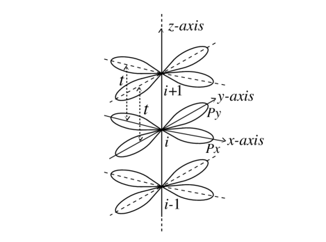
FIG. 1.: A one-dimensional Hubbard model with twofold degenerate orbitals at each site.

III Ground state and excitations

To understand the physics of the present model, let us consider $S$ and $T$ spins as classical spins. The spin configurations where every adjacent two, either $S$ or $T$, spins point the opposite direction have the lowest energy. Thus the classical ground state energy is zero and the degeneracy of the ground states is macroscopic in the classical theory. This situation is different from usual orbital and/or spin orderings discussed so far. Thus it is essential to examine the properties of Hamiltonian (9) by unbiased methods.

First, we calculate the ground state energy ($E_{g.s.}$) by the DMRG method[9] in the subspace of $(S_{tot}^{z},T_{tot}^{z})$=(0,0), where $S_{tot}^{z}\equiv\sum_{i}S_{i}^{z}$ and $T_{tot}^{z}\equiv\sum_{i}T_{i}^{z}$. We take $K=1$ as the energy unit and use here the open boundary conditions (OBC) to obtain sufficient accuracy by the DMRG method. The obtained results are shown in Fig. 2, which shows that the ground state energy per site ($E_{g.s.}/N$) and the surface energy are equal to $-$0.825 and 0.35(3), respectively. This ground state energy is, of course, consistent with that obtained by the Bethe ansatz, $E_{g.s.}/N\simeq-0.825\,12$ [8].

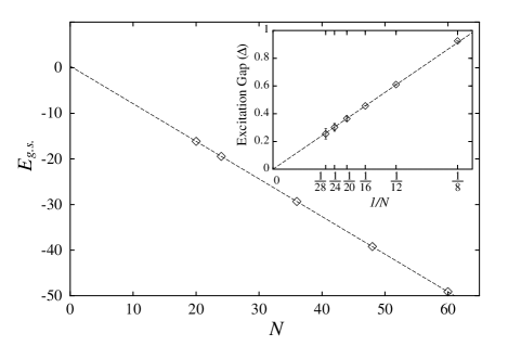
FIG. 2.: Ground state energy as a function of $N$. The numerical errors, which are estimated from the truncation errors in the DMRG calculation, are less than 0.01%. The broken lines represent the linear fitting; $E_{g.s.}=-0.825\times N+0.35(3)$. The inset shows the excitation gap ($\Delta$) as a function of $1/N$. Error bars are estimated from the truncation errors in the DMRG calculation. The dotted line represents the linear fitting, $\Delta=7.3/N$

In Fig. 2 the ground state energies are plotted only for $N=4n$, for which the minimum energy in the subspace of $(S_{tot}^{z},T_{tot}^{z})$=(1,1) is different from $E_{g.s.}$. From Table I it is seen that the subspace $(S_{tot}^{z},T_{tot}^{z})$=(0,0) is included in every irreducible representation, but $(S_{tot}^{z},T_{tot}^{z})$=(1,1) belongs to any irreducible representation except for $[1^{4}]$. Thus it is concluded that the ground state belongs to the $[1^{4}]$ irreducible representation in the Young’s diagram notation. Similarly, by calculating the ground state energies with changing $(S_{tot}^{z},T_{tot}^{z})$, it is found that for $N=4n+2$ the ground states belong to either $[2^{3}]$ or $[2^{2}1^{2}]$, which are degenerate 10- and 6-fold, respectively (see Table I).

These quantum numbers can be understood from the point of view of maximum antisymmetrization. That is, the irreducible representations thus obtained for the ground states are compatible with the simple fact that the more antisymmetric part one irreducible representation has, the lower is its ground state energy in the subspace, because the Hamiltonian (9) is the sum of SU(4) exchange operators. To avoid complications coming from the degenerate ground states, we consider the systems of $N=4n$ in the following. In this case the ground state belongs to the $[1^{4}]$ and is a singlet. Since the Lieb-Schultz-Mattis theorem applies to this model, the excitations are expected to be gapless, provided that no other symmetry is broken, in the same way as the spin-1/2 AF Heisenberg model with SU(2) symmetry.

To estimate the excitation energy, we calculate the ground state energy and the first excited state energy by using the DMRG method for $N\geq 20$ and by the exact diagonalization (Lanczos method) for $N\leq 16$. We determine the ground state energy and the first excited energy by the minimum energies of the states whose quantum numbers $(S_{tot}^{z},T_{tot}^{z})$ are specified: $(0,0)$, $(1,1)$, etc. It is found that the first excited state belongs to $[2^{1}1^{2}]$.

Though the DMRG is more suitable for OBC than periodic boundary conditions (PBC), here we apply the PBC in order to study the properties in the bulk limit. When we use the OBC, we get lower excitation energies than those shown in the inset of Fig. 2, but they correspond to excitations at the surfaces rather than those in bulk. From the inset of Fig. 2 we can conclude that the excitation gap $(\Delta)$ goes to zero as $\Delta\sim 7.3/N$.

In order to examine the properties of the excitations in more detail, we calculate the dispersion relation by using the Lanczos method with the use of translational symmetry for the systems with the PBC. Figure 3 shows that the excitation spectrum has a “bactrian camel” structure and shows softening at $q=\pi/2$. This structure is also known by the Bethe ansatz results [8]. Corresponding to the softening at $q=\pi/2$, the correlation functions would show a characteristic feature, namely, oscillatory behaviors with a period of four, which we will discuss in the next section.

Figure 3 shows that height of the left hump is always lower than that of the right one. To consider a possible reason, we determine the irreducible representation of each state for $N=8$ and $12$. Quantum numbers assigned for each $q$ point in the dispersion curves are shown in Fig. 3 by the SU(4) Young’s diagram representations. In these finite size calculations, the state at $q=\pi/2$ and left part of the two humps always belongs to $[2^{1}1^{2}]$ and the right one to $[3^{1}1^{1}]$. From Table I, the first excited states at $q=\pi/2$ consist of the coupled spin and orbital excitations in addition to the pure spin and orbital excitations and have the $15\!\times\!2$-fold degeneracy in total. The difference of the height of the two humps may be attributed to the difference of the irreducible representations of the two humps. In fact, the left (lower) hump belongs to the irreducible representation which has a more antisymmetric part than that of the right (higher) one. In the bulk limit, however, we expect that the two parts, $0<q<\pi/2\,$ and $\,\pi/2<q<\pi$, converge to the same dispersion relation as is known by the Bethe ansatz solution[8].

TABLE I.: Irreducible representations of the SU(4) symmetry given by Young’s diagrams (YD) and their relations to $(S_{tot},T_{tot})$ and $S^{(3/2)}_{tot}$ representations[9], where $S_{tot}$, $T_{tot}$, and $S^{(3/2)}_{tot}$ are the magnitudes of the ${\vec{S}}_{tot}\equiv\sum_{i}{\vec{S}}_{i}$, ${\vec{T}}_{tot}\equiv\sum_{i}{\vec{T}}_{i}$, and ${\vec{S}}^{(3/2)}_{tot}\equiv\sum_{i}{\vec{S}}^{(3/2)}_{i}$, respectively. Here $\nu$ is the degeneracy of each representations.

YD	$\nu$	$(S_{tot},T_{tot})$	$S^{(3/2)}_{tot}$
$[1^{4}]$	1	(0,0)	0
$[2^{1}1^{2}]$	15	(0,1)$\oplus$(1,0)$\oplus$(1,1)	1$\oplus$2$\oplus$3
$[2^{2}]$	20	(0,0)$\oplus$(1,1)$\oplus$(0,2)$\oplus$(2,0)	0$\oplus$2$\oplus$2$\oplus$4
$[3^{1}1^{1}]$	45	(0,1)$\oplus$(1,0)$\oplus$(1,1)$\oplus$(1,2)$\oplus$(2,1)	1$\oplus$1$\oplus$2$\oplus$3$\oplus$3$\oplus$4$\oplus$5
$[4^{1}]$	35	(0,0)$\oplus$(1,1)$\oplus$(2,2)	0$\oplus$2$\oplus$3$\oplus$4$\oplus$6
$[2^{2}1^{2}]$	6	(1,0)$\oplus$(0,1)	0$\oplus$2
$[2^{3}]$	10	(0,0)$\oplus$(1,1)	1$\oplus$3

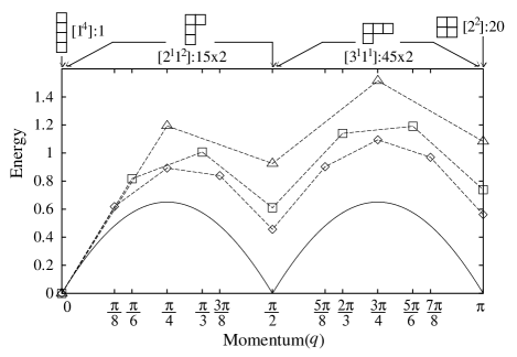
FIG. 3.: Dispersion relations. The symbols $\triangle$, $\Box$, and $\Diamond$ represent data for $N=8$, 12, and 16, respectively. Young’s diagrams (YD) show the irreducible representations. The numbers accompanied by YD show the degeneracy and $\times 2$ represents the same weight from $q$ and $-q$. The solid line represents the Bethe ansatz result[7].

IV Correlation Functions

Now we move on to the behaviors of the correlation functions, $\langle{S}^{z}_{i}\cdot{S}^{z}_{i+j}\rangle_{g.s.}$, where $\langle\cdots\rangle_{g.s.}$ denotes expectation values for the ground state. Since Hamiltonian (8) has rotational symmetry with respect to both $S$ and $T$ spins, we consider only $z$ components of spins.

We use the OBC to get better accuracy in the DMRG calculations, but in this case we must keep in mind that the data contain the effects from boundaries. $\langle S^{z}_{i}\cdot S^{z}_{i+j}\rangle_{g.s.}$ shows an oscillatory behavior with a period of four as a function of $j$. But the correlation functions also vary with a period of four with respect to $i$. That is, $\langle S^{z}_{i}\cdot S^{z}_{i+j}\rangle_{g.s.}$ is equal to $\langle S^{z}_{i+4}\cdot S^{z}_{i+4+j}\rangle_{g.s.}$ for any $i,j$.

This behavior is caused by the standing wave with a period of four originating from the open boundaries. To remove such an artifact due to the OBC, we average $\langle S^{z}_{i}\cdot S^{z}_{i+j}\rangle_{g.s.}$ for one period with respect to $i$. Thus we define an approximate bulk correlation function as follows:

$$\langle S^{z}_{i}\cdot S^{z}_{i+j}\rangle_{bulk}\equiv\frac{1}{4}\sum_{k=0}^{3}\langle{S}^{z}_{i+k}\cdot{S}^{z}_{i+k+j}\rangle_{g.s.}\quad.$$ (10)

After this averaging procedure, we get the natural behavior of the correlation functions as shown in Fig. 4 .

Because the results discussed in the previous section show that this model is gapless, we try to fit the envelope of $\langle S^{z}_{i}\cdot S^{z}_{i+j}\rangle_{bulk}$ data with a power-law function ( $j^{-\alpha}$) by the least mean square method and get critical exponent $\alpha$ equal to 1.80 or 1.55 depending on using either the upper ($j=12,$ 16, and 20) or the lower ($j=14$, 18, and 22) data. We did not use the data of $j=24,26$ and $28$, because these sites are too close to the boundary. Due to finite size effects, the value of $\alpha$ depends on how to fit, but $\alpha$ is always between 1.5 and 2.0. From these results, we conclude that the asymptotic form of the correlation function is given by

$$\langle{S}^{z}_{i}\cdot{S}^{z}_{i+j}\rangle_{bulk}\sim\frac{\cos{(\frac{\pi}{2}j)}}{j^{\alpha}};\quad\alpha=1.5-2.0,$$ (11)

in the bulk limit.

Of course, $\langle S^{z}_{i}\cdot S^{z}_{i+j}\rangle_{bulk}$ is equal to $\langle T^{z}_{i}\cdot T^{z}_{i+j}\rangle_{bulk}$, because of the symmetry of Hamiltonian (8) concerning the exchange between ${{\vec{S}}}$ and ${{\vec{T}}}$. Furthermore, $\langle S^{z}_{i}\cdot T^{z}_{i+j}\rangle_{bulk}$ always equals zero as is easily shown by the Wigner-Eckart theorem. In fact, the calculated values of $\langle S^{z}_{i}\cdot T^{z}_{i+j}\rangle_{bulk}$ are almost zero, and the numerical errors for the values of $\langle S^{z}_{i}\cdot S^{z}_{i+j}\rangle_{bulk}$ may be estimated from these values, which are less than $1\%$ even at the farthest site from $i$.

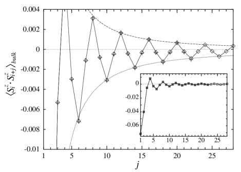
FIG. 4.: Correlation functions ($\langle S^{z}_{i}\cdot S^{z}_{i+j}\rangle_{bulk}$) for the systems with $N=48$ ($+$) and $60$ ($\Diamond$). Broken and dotted lines are $0.144/j^{1.80}$ and $-0.108/j^{1.55}$, which are the results of the least mean square fitting using the upper and lower data, respectively. Numerical errors, which are estimated from the values of $\langle S^{z}_{i}\cdot T^{z}_{i+j}\rangle_{bulk}$, are less than 1%. The inset shows the entire form of the correlation functions. The symbols $\times$ and $\Box$ represent data for $N=48$ and $60$, respectively, but they overlap nearly perfectly.

Next we study the structure factor defined by

$$S^{z}(q)\equiv\sum_{j=-N/2+3}^{N/2-2}\langle S^{z}_{i}\cdot S^{z}_{i+j}\rangle_{bulk}\cdot e^{-iqj}\quad.$$ (12)

As is seen in Fig. 5, $S^{z}(q)$ has a characteristic cusp structure at $q=\pi/2$. This result is consistent with the softening at $q=\pi/2$ in the dispersion relation. By Fourier transformation of Eq. (11), the analytic form of $S^{z}(q)$ is given by

$$S^{z}(q)\sim S^{z}(q=\frac{\pi}{2})-\frac{\pi}{2}\frac{|q-\frac{\pi}{2}|^{\alpha-1}}{{\it{\Gamma}}(\alpha)\sin{\frac{\alpha-1}{2}\pi}}+O\left(q-\frac{\pi}{2}\right)$$ (13)

around $q=\pi/2$, when $1<\alpha<3$. If $\alpha$ is greater than 2, Eq. (13) does not show any cusp structure at $q=\pi/2$. So $\alpha$ must be less than $2$, since we clearly see the cusp structure of $S^{z}(q)$ which becomes sharper as the system size is increased.

By the SU(4) conformal field theory, the critical exponent of the SU(4) spin correlation functions with $q=\pi/2$ oscillations is obtained to be 3/2[11], which is consistent with the present numerical result. Although the correlation functions discussed in this paper are the $S$-spin correlation functions but not the SU(4) spin correlation functions, we can show that the exponent is the same for the two correlation functions.

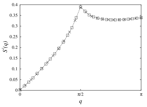
FIG. 5.: Fourier transformation of the correlation function for the systems with $N=60$ ($\Box$) and $N=48$ ($\times$).

V Conclusions and discussions

In conclusion, we have studied the quantum critical state for the coupled spin-orbit system. The quantum numbers of the ground state and the lowest branch of the excitations are determined. Furthermore, the spin-spin correlation functions are obtained explicitly for the first time by the DMRG method. It shows a power-law decay with a period of four, which originate from the interference between the spin and orbital degrees of freedom. The exponent of the asymptotic behavior is consistent with the prediction by the conformal field theory.

In this paper we have investigated only the most symmetric model, but it is more realistic to consider a model with lower symmetry corresponding to a finite $J$. In such a case the effective Hamiltonian is given by the $S$-spin isotropic and $T$-spin Ising-type Hamiltonian (7), whose properties are not yet fully understood.

Related to the SU(4) model, several models with lower symmetries have been studied[12, 13, 14]. Kawano and Takahashi[13] discussed $S$-spin isotropic and $T$-spin $XY$-type Hamiltonians to study the three-leg antiferromagnetic Heisenberg ladder and showed that such a model is gapfull and has exponentially decaying correlation functions. Kolezhuk and Mikeska[14] studied a special SU(2)$\times$SU(2) symmetric Hamiltonian $\sum_{i}({\vec{S}}_{i}\cdot{\vec{S}}_{i+1}+3/4)({\vec{T}}_{i}\cdot{\vec{T}}_{i+1}+3/4)$ and showed that this model is also gapfull.

It may be possible to study the properties of these models in a unified way by introducing different type of anisotropies from the SU(4) symmetric point. For this purpose, it is highly desirable to develop an analytic theory around this symmetric point.

REFERENCES

- [1] Present address: Institute of Applied Physics, University of Tsukuba, Tsukuba 305, Japan.
- [2] K. I. Kugel and D. I. Khomskii, Sov. Phys. JETP 37, 725 (1973) [Zh. Eksp. Teor. Fiz. 64, 1429 (1973)].
- [3] S. Inagaki, J. Phys. Soc. Jpn. 39, 596 (1975).
- [4] R. Shiina, H. Shiba, and P. Thalmeier, J. Phys. Soc. Jpn. 66, 1741 (1997).
- [5] J. des Cloizeaux and J. J. Pearson, Phys. Rev. 128, 2131 (1962).
- [6] E. H. Lieb, T. Schultz, and D. J. Mattis, Ann. Phys. (N.Y.) 16, 407 (1961).
- [7] I. Affleck and E. H. Lieb, Lett. Math. Phys. 12, 57 (1986).
- [8] B. Sutherland, Phys. Rev. B 12, 3795 (1975).
- [9] S. R. White, Phys. Rev. Lett. 69, 2863 (1992).
- [10] X. Hamermesh, Group Theory, (Addison-Wesley, Reading, MA, 1962).
- [11] I. Affleck, Nucl. Phys. B 265, 409 (1986).
- [12] N. Shibata, M. Sigrist, and E. Heeb, Phys. Rev. B 56, 11084 (1997).
- [13] K. Kawano and M. Takahashi, J. Phys. Soc. Jpn. 66, 4001 (1997).
- [14] A. K. Kolezhuk and H.-J. Mikeska, Phys. Rev. Lett. 80, 2709 (1998).
- [15] Y. Q. Li, Michael Ma, D. N. Shi, and F. C. Zhang, cond-mat/9804157 .