Formation of helical states in wormlike polymer chains

Abstract

We propose a potential for wormlike polymer chains which can be used to model the low-temperature conformational structures. We successfully reproduced helix ground states up to 6.5 helical loops, using the multicanonical Monte Carlo simulation method. We demonstrate that the coil-helix transition involves four distinct phases: coil(gaslike), collapsed globular(liquidlike), and two helical phases I and II (both solidlike). The helix I phase is characterized by a helical structure with dangling loose ends, and the helix II phase corresponds to a near perfect helix ordering in the entire crystallized chain.

The structure of $\alpha$-helices is one of the most common conformations occurring in biological molecules such as proteins. It is this unique structure that acts as the building block for much more complicated tertiary structures [1]. In 1959, Zimm and Bragg proposed a mean-field model for the coil-helix transition that was based on the thermodynamics of a known sequence of pairing residues[2]. A tremendous number of theoretical works have been published since then and the basic approaches are derivatives or alterations of the original Zimm-Bragg treatment [3, 4]. Most recent numerical attempts to study the problem are based on more realistic potentials at the atomic level for helix-forming polypeptides, concentrating more on finding the ground state structure [5], than on the thermodynamics at finite temperatures (see, however, Ref. [6]).

From the statistical-physics perspective, it is desirable to start from a simple theoretical model of general characteristics, in the same sprite as recent models for double stranded semiflexible polymers [7], for low-temperature lattice homopolymers [8] and for polymer chains containing dipolar segments [9]. By ignoring the specifics of the amino acids, most proteins can be viewed as wormlike polymer chains. One can then ask simple questions such as, what are the minimum conditions required for a wormlike polymer chain to reproduce a helix ground state? What are the characteristics of the so-called coil-helix transition in comparison with the predictions of a Zimm-Bragg-type theory, and how different is it from the coil-collapsing transition in other polymeric molecules occurring near the theta temperature? From a polymer physics point of view, a related and inspiring question by itself is: what are the low temperature structures of a wormlike polymer chain in general?

There are two basic characteristics common to all wormlike chains: the existence of a finite persistence length, which prevents the polymer from folding as a sharp hairpin loop at scales smaller than the persistence length, and an excluded volume interaction between the monomers, which prevents polymer chains from collapsing into a point at low temperatures. For helix-forming wormlike polymers, a third basic characteristic must be included: a directionally biased attractive potential.

In the current approach we model wormlike polymers by fixing the bond angle $\theta$ between two adjacent polymer bonds of length $a$, and allowing the azimuthal angle $\phi$ rotate freely, as prescribed in the original freely rotating model [10]. Movement of monomers is realized by implementing a pivot algorithm [11], where a bond is chosen at random as a reference axis about which the entire polymer segment attached to this bond is rotated. The Metropolis method of sampling a canonical phase space is known to be ineffective for examining the possible conformational states at low temperatures, as a particular configuration could easily become trapped in a local energy minimum. To avoid this problem we have incorporated a multicanonical technique into the pivot algorithm, which involves reweighting the temperature as a function of energy, in order to produce a flat simulation histogram across the entire energy landscape [5, 12]. This approach allows the polymer to potentially visit all possible energy states and to tunnel through local energy minima. For a more detailed explanation of the multicanonical technique the reader is referred to Refs [6, 12].

The interaction energy between the monomers labeled $i$ and $j$ having a center-to-center distance $r_{ij}$ is proposed to have the simple form,

$${V}_{ij}=\cases{0&${\rm for~{}}\sigma\leq r_{ij}$\cr{-\epsilon[{\vec{u}}_{i}\cdot({\vec{r}}_{i}-{\vec{r}}_{j})]^{m}-\epsilon[{\vec{u}}_{j}\cdot({\vec{r}}_{i}-{\vec{r}}_{j})]^{m}}&${\rm for~{}}d\leq r_{ij}\leq\sigma$\cr\infty&${\rm for~{}}0\leq r_{ij}\leq d$\cr}$$ (1)

where $\vec{u}_{\rm i}$ is the cross product defined as

$$\vec{u}_{\rm i}=(\vec{r}_{\rm i}-\vec{r}_{\rm i-1})\times(\vec{r}_{\rm i+1}-\vec{r}_{\rm i}).$$

Here, $m$ represents the degree of directional bias in the potential, $d$ is the excluded-volume diameter, and $\sigma$ is the attractive-force range. The multicanonical technique is also an effective method to search for the ground states of a given potential. In an effort to answer the question of what type of potential is needed for the creation of a perfect helical ground state, the consequences of using various values of $m$ were examined. We found that for an isotropic interaction ($m=0$), the stable ground state structure is a disordered globular state with no particular relative directional ordering between the chain bonds. Thus, a directionalized interaction ($m\neq 0$) is obviously an essential condition for a helix-forming wormlike chain. We also found that weaker powers ($m=2,4$), would only produce a perfect helix ground state in short polymers; in longer polymers multiple bonds formed by spooling around a helix core i might give rise to an even lower energy. In a helix state, bonding effects should be maximized when all monomers siting directly on top of each other, demanding a strongly directionalized interaction potential as in known helix-forming polypeptides. As an illustration of some of the specific physical properties of a helix-forming wormlike chain, we report here the case of $m=6$ only. Numerical data collected on using other power $m$ will be reported elsewhere.

It is worth noting that our potential is not simply a function of the distance between the two involved monomers. The bonding preference also involves the directions of the bonds connected to these two monomers, which is an interesting effect in the transition to the helix states, similar to a protypical hydrophobic interaction in proteins. There are a number of other variables in the potential model. The diameter $d$ and constant $\sigma$ have been adjusted to have the values $3/2a$ and ${\sqrt{45/8}}a$, while the nearest neighbor interaction is ignored. The fixed bond angle $\theta$ is chosen to have a value of approximately $\pi/3$, corrected for the helical pitch to maintain six monomers per helix loop. These selections of values were based on the observation that under the current choice a stray end of the monomers cannot loop through an open core of a partially formed helical segment. We have also investigated the case of $\theta=\pi/5$, and found no major qualitative differenced in the physical properties to be examined below. This choice of potential, with the use multicanonical technique, was able to produce a perfect helical ground state relatively quickly (see Fig 1d) for various polymer lengths $N=13,19,26$ and $39$, showing that the helix ground state can be constructed with the above mentioned three conditions of a helix-forming wormlike chain.

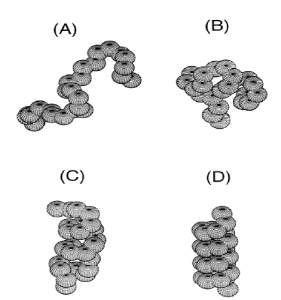
FIG. 1.: Snapshots of the configurations of a 26mer at various temperatures: (a) $k_{B}T/\epsilon=4$ (coil), (b) $k_{B}T/\epsilon=1.3$ (globular) (c) $k_{B}T/\epsilon=0.8$ (helix I) and (d) $k_{B}T/\epsilon=0.1$ (helix II). The size of the beads represents the actual hard-core interaction between non-adjacent monomers, and the attraction force range is ${\sqrt{5/2}}a$, where $a$ is the bond length. A highly directionalized potential with $m=6$ (see Eq. (1)) is used.

Therefore, a wormlike chain can have numerous types of ground states, which are dependent on the type of directional potential used. The construction a potential which produces a singular ground state of a desired conformation is possible, although not a trivial exercise. The use of multicanonical technique makes the search for these specific ground states simpler. Knowing that our model has an attainable perfect helix ground state, we have calculated the multicanonical reweighting function for the temperature range discussed below, which enable us to conduct measurements of physical quantities in the subsequent production runs. As a most effective measure for exploring the phase transition signatures, the specific heat capacity of the polymer chain was calculated by measuring the energy fluctuations

$$C_{v}/k_{B}={{\langle E^{2}\rangle-\langle E\rangle^{2}}\over{(k_{B}T)^{2}}}$$

The mean square radius of gyration,

$$<R_{\rm g}^{2}>=<{1\over N}\sum_{i=1}^{N}(\vec{r}_{\rm i}-\vec{r}_{\rm cm})^{2}>$$

where $\vec{r}_{\rm cm}$ is the center of mass vector, and the mean square end to end distance,

$$<R_{\rm end}^{2}>=<(\vec{r}_{\rm 1}-\vec{r}_{\rm N})^{2}>$$

were also calculated to characterize the spatial dimension the polymer chain. Finally we introduced three parameters to measure the degree of helicity within the chain. This is accessed in many references by examining the Ramachandran angles $\phi$ and $\psi$ which are parameters not present in our current model. Equivalent to the same treatment, the first helicity parameter, $H_{1}$, is based on an examination of the distance between the $i^{th}$ and $(i+3)^{th}$ monomers, which is calculated and evaluated as being in a helical or non-helical state, as the three connected bonds in the segment will be arranged in a very specific way when in the helix state. A window of allowed distances can then define a three-monomer segment as helical, and the average number of helical segments, $H_{\rm 1}$, can be measured. A second method of characterizing the degree of local helicity within the polymer involves summing the dot products of the adjoining cross products of connected bond vectors:

$$H_{\rm 2}={1\over N-2}\sum_{i=2}^{N-1}(\vec{u}_{\rm i}\cdot\vec{u}_{\rm i+1})$$

A third measurement is the correlation function $G(i)\equiv{\vec{u}_{i}}\cdot{\vec{u}}_{\rm mid}$, where $\vec{u}_{\rm mid}$ corresponds to the vector in Eq. (2) for the central monomer, characterizing the correlation of the helical ordering along the chain. Discussed below is the integrated correlation function,

$$H_{\rm 3}={1\over N-2}\sum_{i=2}^{N-1}(\vec{u}_{\rm i}\cdot\vec{u}_{\rm mid})$$

which represents the averaged correlation in the chain. These three parameters yield a global representation of the amount of helicity in the polymer.

Using the reweighting function from preliminary deterministic multicanonical runs, we performed a typical production run of $5\times 10^{8}$ pivot rotations with measurement made every 10 steps for rescaled temperatures $k_{B}T/\epsilon$ ranging from 0.1 to 5.0. Polymer chain lengths of 13,19,26, and 39 monomers were considered and the results are shown in Fig. 2.

Displayed in Fig. 2a, the scaled heat capacity curves shows a number of interesting features. The first and most obvious is the large peak near $kT/\epsilon=1.2$ corresponding to the transition to a helix state. The words describing what is meant by a helix state must be chosen carefully for the reason that there are two distinct helix states observed in this study. Figures 1b and 1c are typical configurations just before and after the transition. Corresponding to a significant increase in the three helical parameters measured for $N=19$ (Fig. 2c), a $C_{v}$ anomaly occurs at this temperature, confirming that the polymer is making a transition from a disordered (Fig. 1b) state to the more ordered helical state (Fig. 1c). The same sharp increase in $C_{v}$ was also predicted in the Zimm-Bragg theory [2, 1] and its variations, and in recent MC simulations by Okamoto and Hansmann [6]. Zimm and Bragg argued that this peak does not represent a second order transition in consistent with the known conclusion regarding the impossibility of phase transitions in a one dimensional system. However, one can also argue that a helix polymer is not strictly a one dimensional system. Our peaks in heat capacity curves continuously increase as $N$ grow, which show a similar behavior as heat capacity curves in a protypical second order phase transition, and qualitatively agree with the observation in a more realistic polypeptide model for shorter helical loops [6]. It would be interesting to further examine a possible finite size scaling in the $C_{v}$ peak values determined from our simulations. However, currently, the main obstacle to achieving this goal is the increasing computational time for larger $N$.

One of the most interesting features of Fig. 2a is the previously unknown second transition occurring in the neighborhood of scaled temperature $k_{B}T/\epsilon=0.3$. In a recent study of the phase transitions in isotropic homopolymers with specific ground states in a lattice model, Zhou et al. [8] have observed a similar transition, and have suggested that this is a solid-solid transition accompanying the crystallization of their polymers into the ground state. In the present case, our wormlike chains have the specifically constructed ground state of a perfect helix, and we believe that the second transition corresponds to the crystallization of the helix I state into a perfect helix II state. Above this transition we have observed that the chain is in a highly ordered helical structure only segmentally as demonstrated by Fig. 1c. In particular, the end portion of the polymer may not necessarily ordered. Even for the ordered segments, elongation motion and bending of the ordered segment as a whole would make the directional ordering weaker compared with the more tightly wound helix II. Thus, as the temperature continues to drop further, the few unbonded end segments arrange themselves into a perfect helical state (helix II), and in the mean time, the already existing helix segments crystallize to a near ground-state structure, shown in Fig. 1d. Such a crystallization transition has not been seriously modeled by previous theoretical studies, which usually treat the helix I to helix II transition as a smooth crossover with no anomalies in the heat capacity, as a result of influence by Zimm-Bragg’s original model [1, 2, 3, 4, 13]. The three lower curves in Fig. 2c are derivatives of the helical parameters, all showing a significant change in the slope corresponding to the low-temperature peak at the $C_{v}$ curve. To further confirm this crystalline transition we have examined individual local the helical parameters ${\vec{u}}_{i}\cdot{\vec{u}}_{i+1}$, which also show substantial changes before and after the helix I to helix II transition. As $N$ becomes large, the peak position in $C_{v}$ seems to be to move to higher temperatures, with the $C_{v}$ curves becoming flatter. Presently, we are unable to confirm these trends due to the large error bars associated with the low temperature behavior.

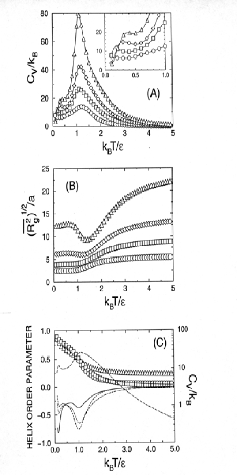
FIG. 2.: Variation of physical quantities as a function of scaled temperature $\tilde{T}=k_{B}T/\epsilon$. Triangles, diamonds, squares, and circles in Figs 2(a) and 2(b) corresponds to 39mers, 26mers, 19mers, and 13mers respectively. Only every tenth data point was plotted, and more data points are represented by the more smooth curves. The error bars of the $C_{v}$ curve are almost twice the size of the plotted symbols, and triple the size of the plotted symbols in the inset. Triangles, squares and circles in Fig 2(c) represents the helix parameters $H_{1}$ , $H_{2}$ and $H_{3}$ for the case of 19mers, respectively. The solid, short-dashed, and the dot-dashed curves represent $dH_{1}/d\tilde{T}$, $dH_{2}/d\tilde{T}$, and $dH_{3}/d\tilde{T}$ respectively. An overlay of the $C_{v}$ curve (to the right scale) is also shown by the long-dashed curve for reference.

Returning to Fig. 2a, we would like to point out a third feature of interest, which is the emergence of a shoulder in the larger polymers near $k_{B}T/\epsilon=2$, not easily detectable from Fig. 2a. This shoulder corresponds to a $\theta$ temperature collapsing of the polymer chain from a gyrated coil (“gaslike”) to a randomly collapsed globular state (“liquidlike”). This collapsing is a direct cause of the directionally averaged attractive potential between the monomers, creating globular states which have little helical ordering. In Fig. 2b, the radius of gyration curves shows a significant decrease near a transition temperature $k_{B}T/\epsilon=2$, as the signature of a collapsing transition in polymers. At lower temperatures, as helix states start to form, there is an increase in both $R_{g}$ and $R_{\rm end}$ (not shown). Such a turnover is actually a characterization of the helix formation, because in a large polymer, the ordered helix structure will be quite extended along the helix axis, forcing the monomers to have an average radius of gyration larger than that of a compact collapsed state. For shorter helices, the increase of polymer dimensions at low temperature does not exist, and the coil-globular and globular-helix I transitions merge to a single transition. Note that neither dimensional parameters show appreciable changes at the helix I-helix II transition, which is again consistent with our belief that the helix I to helix II transition merely involves the ordering of the end segments and tightening of the helix segments, with no significant structural rearrangement.

To summarize, we have described a simple model which can be used for examining the coil-helix transitions. To furnish a stable perfect helix ground state, one employs a strongly directionalized attractive potential. The coil-helix transition actually consists of three steps as the temperature is lowered. At high temperatures the polymer has a gaslike coil conformation which collapses into a liquidlike globular conformation with the relative bond directions still remain disordered. This state then makes a transition to a relatively well ordered “solid”-like helix I state, with a dramatic increase in bond direction correlation. Upon further cooling this conformation crystallizes to the very well ordered helix II state. It would be interesting to confirm that this transition indeed accompanies a $C_{v}$ anomaly experimentally in short polypeptide chains which are known to exhibit perfect helical ground states. We hope the current model will shed some light on analyzing experimental data in complimentary to a traditional Zimm-Bragg type physical picture. We believe that the current treatment can be modified with little effort to produce a variety of ground states, important to modeling other interesting transitions in biological systems.

It is a pleasure to acknowledge insightful conversations with B. Nickel, D. Sullivan and P. Waldron, the help of C.Z. Cai on plotting Fig. 1, as well as the financial support of this work by the Natural Sciences and Engineering Research Council of Canada. We would also like to thank M. Gingras for generous CPU time allocation on his Sun Enterprise 450 workstation.

REFERENCES

- [1] See, for example, D. Poland, H.A, Scheraga, Theory of Helix-Coil Transitions, Academic Press, New York, 1970; J.M. Scholtz and R.L. Baldwin, Annu. Rev. Biophys. Biomol. Struct. 21, 95 (1992)
- [2] B.H. Zimm, J.K., Bragg, J. Chem. Phys., 30, 271 (1959).
- [3] See, for example, K. Nagai, J. Phys. Soc. Jpn, 15, 407, (1961); S. Lifson, A. Roig, J. Chem. Phys., 34, 1963 (1961); V. Madison, J. Schellman, Biomolecules, 11, 1041 (1972); Also see reference cited in Ref. [1].
- [4] H. Qian and J. A. Schellman, J. Phys. Chem. 96, 3987 (1992); H. Qian, Biophysical Journal 67, 349 (1994).
- [5] S.-S. Sung, Biophys. Journal 68, 826 (1995); D.R. Ripoll, and H.A. Scheraga, Biopolymers 27, 1283 (1988); S.R. Wilson and W. Cui, Biopolymers, 29, 225 (1990); H. Kawai, Y. Okamoto, M. Fukugta, T. Nakazawa, and T. Kikuchi, Chem. Lett. 2, 1991; Y. Okamoto, Proteins Struct. Funct. Genet. 19, 14 (1994).
- [6] Y. Okamoto, U.H.E Hansmann, J. Chem. Phys. 99, 11276 (1995)
- [7] T.B. Liverpool, R.Golestanian, K. Kremer, Phys. Rev. Lett. 80 (2), 405 (1998)
- [8] Y. Zhou, C.H. Hall, M. Karplus, Phys. Rev. Lett. 77 (13), 2822 (1996)
- [9] M. Muthukumar, J. Chem. Phys. 104 (2), 691 (1995)
- [10] H. Yamakawa, Modern Theory of Polymer Solutions, Harper and Row, New Yrok, (1971).
- [11] N. Madras, A.D. Sokal, J. Stat. Phys. 50, 109 (1988)
- [12] U.H.E Hansmann, Y. Okamoto, Physica A 212, 415 (1994)
- [13] Upon re-examination of the transition curves, obtained by the real potential model of Okamoto and Hansmann [6], an emergence of a second peak is seen in their data, for which is known to be a strong helix former. However, there is no discussion given for its existence in Ref. [6].