Phase Behavior of Binary Fluid Mixtures Confined in a Model Aerogel

Abstract

It is found experimentally that the coexistence region of a vapor–liquid system or a binary mixture is substantially narrowed when the fluid is confined in a aerogel with a high degree of porosity (e.g. of the order of $95\%$ to $99\%$). A Hamiltonian model for this system has recently been introduced [1]. We have performed Monte–Carlo simulations for this model to obtain the phase diagram for the model. We use a periodic fractal structure constructed by diffusion-limited cluster-cluster aggregation (DLCA) method to simulate a realistic gel environment. The phase diagram obtained is qualitatively similar to that observed experimentally. We also have observed some metastable branches in the phase diagram which have not been seen in experiments yet. These branches, however, might be important in the context of recent theoretical predictions and other simulations.

Journal of Sol–Gel Science and Technology ??

?? ?? 1998

?? ??

1 Introduction

When a simple liquid or a binary mixture is confined in a porous material which has a very low density ($1$–$5\%$) of spatially fixed impurities, such as in an aerogel, the coexistence region in the phase diagram is substantially narrowed. This result has been obtained in a broad class of experimental studies, such as vapor–liquid coexistence of ⁴He[2] and Nitrogen[3], binary mixtures of isobutyric acid–water[4] and ³He–⁴He[5], etc. In all of these studies, the coexistence curve was shown to change dramatically when the system was confined in a low concentration silica aerogel.

Recent theoretical efforts have been aimed to understand the above mentioned behavior. These include mean–field type studies of the Random Field Ising model[6], a liquid state approach using the Ornstein–Zernike equations[7] and numerical simulations of a modified version of the Blume–Emery–Griffiths model[8]. A very successful approach was initiated by Donley and Liu[1]. In this reference, the authors introduce a free energy functional that takes into account the interactions that arise from the contact between the system molecules and the aerogel. By minimizing this free energy they obtain a coexistence curve which is in rough qualitative agreement with the experimental results. Moreover, the authors go beyond this mean field type approach by using a parametric form of the equation of state, combined with linear interpolation techniques. Although this new approach yields better results than the previous mean field treatment, it is not conclusive since other parametric models may give different results. Moreover, as the authors point out correctly, it is very important to study the role of the fluctuations.

In this paper, we go beyond the mean field approach and numerically determine the phase diagram of the model introduced in [1] by using Monte Carlo methods. In this model, one considers a scalar field $m({\bf r})$ and writes down a Hamiltonian which includes bulk terms plus surface terms coming from the interaction with the aerogel:

$${\cal H} = \int_{V}dV\left[\frac{\theta}{2}m^{2}({\bf r})+\frac{\chi}{4}m^{4}({\bf r})\right.$$ (1)

$$\left.-Hm({\bf r})+\frac{1}{2}|\nabla m({\bf r})|^{2}\right]$$

$$+\oint_{S}dS\left[-H_{1}m({\bf r})+\frac{{\cal G}}{2}m^{2}({\bf r})\right]$$

The bulk terms, the first volume integral, is the usual Ginzburg–Landau model for a scalar concentration field $m({\bf r})$ used in binary phase–transitions. The additional term given by the surface integral represents the superficial stress[9] in the neighborhood of gel. Here, the volume $V$ is the available volume for the fluid and the surface $S$ is the set of fluid points in contact with the gel. The parameters for this model are: $\theta$, which is related to the temperature; $\chi$ which sets the width of the coexistence curve; the external field (playing the role of the chemical potential) $H$; the surface field $H_{1}$; and the surface enhancement parameter ${\cal G}$.

We have performed Monte–Carlo simulations of the lattice version of the above Hamiltonian in order to find its phase diagram. We consider a three-dimensional simple cubic lattice with periodic boundary conditions. In this lattice, we simulate the presence of the aerogel by considering that $N_{G}$ out of the $L^{3}$ lattice sites belong to a gel structure generated in a way to be explained in detail later. We call these sites “gel sites”. In the remaining sites (the “field sites”) we consider the scalar variable $m_{i}$ ($i=1,\dots,N=L^{3}-N_{G}$) representing the fluid density field. The gradient term of eq.(1) is discretized in the usual way:

$$|\nabla m({\bf r})|^{2}\rightarrow\sum_{\mu=1}^{3}(m_{i}-m_{i_{\mu}})^{2}$$ (2)

where $(i_{1},i_{2},i_{3})$ stands for the set of right–nearest–neighbors sites to site $i$. However, the presence of the gel has the effect that in this expression for the gradient: only those neighbor sites which are actually field sites contribute to the sum. Accordingly, we introduce a set of indexes, $O_{i_{\mu}}$ defined to be equal to 1, when the site $i_{\mu}$ is a field site, or 0, when the site $i_{\mu}$ is a gel site. The gradient term becomes then:

$$|\nabla m({\bf r})|^{2}\rightarrow\sum_{\mu=1}^{3}O_{i_{\mu}}(m_{i}-m_{i_{\mu}})^{2}$$ (3)

For the sake of clarity in notation we have ordered the $N$ field points such that, from $1$ to $N_{B}$ we have “pure bulk” field sites (i.e. those which are not in contact with the gel) and from $N_{B}+1$ to $N$ we have $N_{S}$ “surface” field sites, (i.e. those in contact with the gel, $N_{S}=N-N_{B}$). With this convection in mind, the lattice version of the Hamiltonian (eq.(1)) can be written as:

$${\cal H} = \sum_{i=1}^{N}\left[tm_{i}^{2}+um_{i}^{4}-hm_{i}\right.$$ (4)

$$+\left.\frac{1}{2}\sum_{\mu=1}^{3}O_{i_{\mu}}(m_{i}-m_{i_{\mu}})^{2}\right]$$

$$+\sum_{i=N_{B}+1}^{N}\left[-h_{1}m_{i}+gm_{i}^{2}\right]$$

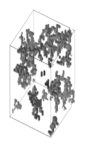
Figure 1: Three dimensional gel structure with a concentration of $4\%$, generated by a realization of the DLCA process, in a lattice with $L=32$ and periodic boundary conditions.

Where, $t$, $u$, $h$, $h_{1}$ and $g$ are parameters obtained by suitable rescaling of the continuum values $\theta$, $\chi$, $H$, $H_{1}$, ${\cal G}$, respectively. The gel sites in this lattice form a periodic fractal structure generated by a diffusion–limited–cluster–aggregation (DLCA) process[10, 11], which mimics the aggregation process that form silica gels. The algorithm proceeds as follows[12]:

Let us consider the starting configuration of the gel as a collection of aggregates (clusters) containing one particle each, the total number of particles is $N_{G}$. At a later time, one obtains a collection of $N_{a}$ aggregates, the $i$-th aggregate containing $n_{i}$ gel particles, so that

$$\sum_{i=1}^{N_{a}}n_{i}=N_{G}$$ (5)

The aggregates evolve in the following way: an aggregate $i$ is chosen at random according to a probability $p_{n_{i}}$ which depends on the number of particles $n_{i}$ that it contains, given by

$$p_{n_{i}}=\frac{n_{i}^{\alpha}}{\sum_{i}n_{i}^{\alpha}}$$ (6)

with $\alpha=-0.55$. Then a space direction is chosen at random among the six possible directions and the cluster is moved by one lattice step in that direction (we use periodic boundary conditions). If the cluster does not collide with any other cluster the algorithm continues by choosing again another cluster at random and moving it. If instead a collision occurs, the two colliding clusters merge into a new cluster formed by sticking together the colliding clusters. The process is repeated until a single cluster remains in the system. The resulting fractal dimension of the clusters is $D_{F}=1.9\pm 0.1$ which is close to the expected value $D_{F}=1/\alpha\approx 1.78$. In Fig.(1), we can see a picture of a fractal gel structure obtained using this DLCA process.

2 The method

We use the average value of the field as the order parameter $\langle M\rangle$:

$$\langle M\rangle=\left\langle\frac{1}{N}\sum_{i=1}^{N}m_{i}\right\rangle$$ (7)

Figure 2: Hysteresis loops, $\langle M\rangle$ versus $h$, for two cases: The gel case ($\diamond$) with a concentration of $c=4\%$ and the no gel case ($+$), both for a parameter value $t=-1.26$. The two vertical lines show the actual value $h$ where the transition take place, in each case, $h=-0.18$ in the gel case, and $h=0$ in the no gel case. Note the presence of little steps in the lower branch in the gel hysteresis loop.

where, for fixed gel structure, averages are performed with respect to the distribution ${\rm e}^{-{\cal H}}$. For a given gel structure representative configurations are obtained by the use of the Monte–Carlo method applied to the lattice Hamiltonian (4). We have used the simple Metropolis algorithm: a field value $m_{i}$ is proposed to change to a new value $m_{i}^{\prime}$ chosen randomly from a uniform distribution in $(m_{i}-\delta,m_{i}+\delta)$ for given $\delta$. The new value $m_{i}^{\prime}$ is accepted with a probability given by $\min[1,{\rm e}^{-\Delta{\cal H}}]$, with $\Delta{\cal H}={\cal H}^{\prime}-{\cal H}$ is the change in the Hamiltonian implied by the proposed change. The order parameter $\langle M\rangle$ is computed as an average over different field configurations. An additional average has been performed with respect to 10 different gel structures.

To find the phase diagram, i.e. the dependence on the “temperature” $t$ of the order parameter $\langle M\rangle$, we take fixed values for the system parameters $u$, $g$ and $h_{1}$, and vary the “temperature” $t$. For each value of the temperature $t$ we compute the hysteresis loop by using the Monte–Carlo method varying the external field $h$ from $+h^{0}$ to $-h^{0}$ and vice-versa. We first start at a sufficiently high value for $h^{0}$ (see later) and compute $\langle M\rangle^{0}$. Next, by keeping the same final configuration for the density field, the external field is lowered by an amount $\Delta^{0}$ to $h^{1}=h^{0}-\Delta^{0}$ and compute the corresponding value for the order parameter $\langle M\rangle^{1}$. Then the field is changed to $h^{2}=h^{1}-\Delta^{1}$ and so on until we arrive at $-h^{0}$. The process is reversed by increasing in a similar way the external field to reach again $+h^{0}$.

In order to determine accurately the hysteresis loop, we do not take a constant value for $\Delta^{i}$ but we take:

$$\Delta^{i}=\Delta^{0}\frac{\Delta^{i-1}}{\sqrt{(h^{i}-h^{i-1})^{2}+(\langle M\rangle^{i}-\langle M\rangle^{i-1})^{2}\alpha^{2}}}$$ (8)

where $\alpha$ is an additional scale control parameter. This means that we control the length along the hysteresis curve allowing us to have smooth hysteresis curves. Two typical results for the hysteresis loops are shown in Fig.(2) for the cases of no gel and a gel filling 4% of the lattice points. In the no–gel case, the hysteresis loop is symmetrical around $h=0$ and one can read directly the equilibrium values for $\pm\langle M\rangle$ by taking the values at $h=0$. When the gel is present, we determine the equilibrium values for $\langle M\rangle$ by demanding that the Gibbs free energy in the two phases is equal. The Gibbs free energy can be obtained by integration of the general relation[13]:

$$\langle M\rangle=-\frac{\partial G}{\partial h}$$ (9)

By integrating along the upper curve of the hysteresis loop we obtain:

$$G^{(1)}(h)=G(h^{0})-\int_{h^{0}}^{h}\langle M\rangle dh$$ (10)

whereas from the lower part of the hysteresis loop:

$$G^{(2)}(h)=G(-h^{0})-\int_{-h^{0}}^{h}\langle M\rangle dh$$ (11)

The equilibrium values for $\langle M\rangle$ are read from the hysteresis loop at the value of the external field $h$ such that $G^{(1)}(h)=G^{(2)}(h)$. In order to compute those values for the free energy, according to (10) and (11) we need to know the values of $G(h^{0})$ and $G(-h^{0})$. For this, we use a sufficiently large value for $h^{0}$. For such a large external field, the mean field is a good approximation, in such a way that the Gibbs free–energy can be replaced by just the internal energy ${\cal H}$. So we take $G(\pm h^{0})\approx{\cal H}(\pm h^{0})$. We have taken $h^{0}=10$. In order to check the validity of mean field for this value of $h^{0}$ we have compared the resulting average $\langle M\rangle^{0}$ obtained in the simulation with the mean field value obtained from minimizing the Hamiltonian ${\cal H}$ for the same value for $h^{0}$. Both results agree within 1%.

In Fig.(3) we plot the results of the numerical integrations (10) and (11) both for the no-gel case and for one gel configuration of porosity 96% for a value of the parameter $t=-1.26$. As expected, in the no gel case, $G^{(1)}(h)$ and $G^{(2)}(h)$ coincide for $h=0$. In the gel case, we read from this curve the corresponding value for $h\approx-0.18$. Using this value, we obtain from the upper and lower curves of the hysteresis loops, see Fig.(2), the corresponding values for $\langle M\rangle$.

We have found that this method can be used efficiently far enough from the critical point. Near the critical point, the numerical errors produce a large uncertainty in the numerical integrations and it is difficult to accurately determine the required value of the external field. In those cases, we have taken simply an average of the lower and upper branches of the hysteresis loop as the values for $\langle M\rangle$. For temperatures above the critical one, there is no hysteresis loop.

Figure 3: The Gibbs free–energy $G(h)$ versus $h$ obtained by integration, Eqs. (10,11), from the hysteresis curves in Fig.(2), in the gel case ($\diamond$) and the no gel case ($+$). From these curves we deduce the necessary value for the external field $h$, where the first-order transition takes place.

3 Phase Diagram

We present in this section the phase diagram as a function of the parameter $t$ for three different cases: (i) the no–gel situation, (ii) a gel case with a porosity of 88% and (iii) a gel case with a porosity of 96%.

Figure 4: Phase diagrams, in the gel ($\diamond$), $c=12\%$, and no gel (continuous line) cases.

We use in all the cases a lattice with $L^{3}=32^{3}$ sites and the common Hamiltonian parameter values $u=0.5$, $h_{1}=4$ and $g=1$. For the factors controlling the step size for the variation of the external field we take $\alpha=3$, $\Delta^{0}=0.05$. The initial values for the hysteresis loop is $h^{0}=10$. In the gel cases, we have taken averages with respect to 10 gel structures. By following the method described in the previous section, we obtain for each temperature two values for the order parameter $\langle M\rangle$. These are plotted in Fig.(4) and Fig.(5) for a porosity of 88% and 96%, respectively. In these figures, we can see clearly the narrowing of the coexistence region when the gel is present. For smaller porosity (larger fraction of the gel) the narrowing is more pronounced as observed in the experiments and in accordance with the results of mean field theory. Although, as mentioned at the end of the previous section, numerical errors become large near the critical point, we conclude from the figures that the critical temperature is lowered when the gel is present. Again, the reduction in the critical temperature is larger for smaller porosity.

Figure 5: Phase diagrams, in the gel ($\diamond$), $c=4\%$, and no gel (continuous line) cases. Note in the gel case that we have included some points ($+$), corresponding to the steps found in the hysteresis loops.

However, we note that in the simulations where the gel is present, we have found some steps in the lower curve of the hysteresis loop, as we can see for instance in Fig.(2), which could be interpreted as signaling a second transition. We have plotted in the phase diagram additional points corresponding to the steps in the hysteresis loops. The location of those points depends strongly on the particular realization of the DLCA process to generate the fractal gel structure. This shows up in the large error bars for these points in the Fig.(5).

The phase diagram obtained in this paper is qualitatively similar to that observed experimentally[2]: the coexistence region in presence of gel is narrowed and shifted with respect to the non–gel situation. There are marks of a second transition which also show up in the mean field studies of reference ([1]) and also in other simulations of the Lennard–Jones fluid[14], although it has not been reported in experimental studies.

- [1] J. Donley and A. Liu. “Phase behavior of near–critical fluids confined in periodic gels”. Phys. Rev. E, 55:539–543, 1997.
- [2] A. Wong and M. Chan. “Liquid–vapor critical point of 4he in aerogel”. Phys. Rev. Lett., 65:2567–2570, 1990.
- [3] A.P.Y. Wong, S.B. Kim, W.I. Goldburg, and M.H.W. Chan. “Phase separation, density fluctuation, and critical dynamics of N2 in aerogel”. Phys. Rev. Lett., 70:954–957, 1993.
- [4] Z. Zhuang, A.G. Casielles, and D.S. Cannell. “Phase diagram of isobutyric acid and water in dilute silica gel”. Phys. Rev. Lett., 77:2969–2972, 1996.
- [5] S.B. Kim, J. Ma, and M.H.W. Chan. “Phase diagram of 3He–4He mixture in aerogel”. Phys. Rev. Lett., 71:2268–2271, 1993.
- [6] A. Maritan, M.R. Swift, M. Cieplak, M.H.W. Chan, and M.W. Cole. “Ordering and phase transitions in random–field ising systems”. Phys. Rev. Lett., 67:1821–1824, 1991.
- [7] E. Pitard, M.L. Rosinberg, G. Stell, and G. Tarjus. “Critical behavior of a fluid in a disordered porous matrix: An Ornstein–Zernike approach”. Phys. Rev. Lett., 41:4361–4364, 1995.
- [8] A. Falicov and A. Berker. “Correlated random–chemical–potential model for the phase transitions of helium mixtures in porous media”. Phys. Rev. Lett., 74:426–429, 1995.
- [9] H. Nakanishi and M. Fisher. “Critical points shifts in films”. J. Chem. Phys., 78:3279–3293, 1983.
- [10] P. Meakin. “Formation of Fractal Clusters and Networks by Irreversible Diffusion–Limited Aggregation”. Phys. Rev. Lett, 51:1119, 1983.
- [11] M. Kolb, R. Botet, and R. Jullien. “Hierarchical model for irreversible kinetic cluster formation”. J. Phys. A, 17:L75, 1983.
- [12] A. Hasmy, E. Anglaret, M. Foret, J. Pelous, and R. Jullien. “Small–angle neutron–scattering investigation of long–range correlations in silica aerogels: Simulations and experiments”. Phys. Rev. B, 50:6006–6016, 1994.
- [13] K. Huang. Statistical Mechanics. John Wiley and Sons, New York, 1987.
- [14] K.S. Page and P.A. Monson. “Phase equilibrium in a molecular model of a fluid confined in a disordered porous material”. Phys. Rev. E, 54:R29–R32, 1996.