Quantum Decoherence and Weak Localization at Low Temperatures

Abstract

We discuss a fundamental effect of the interaction-induced decoherence of the electron wave function in disordered metals. In the first part of the paper we consider a simple model of a quantum particle interacting with a bath of harmonic oscillators and analyze the physical origin of the effect. This exactly solvable model also allows to understand why the arguments against the existence of the effect at low temperatures fail. The second part of the paper is devoted to a rigorous analysis of quantum decoherence in disordered metals. We also discuss the relation of our results to the recent experiments on GaAs structures. The existence of a finite quantum decoherence rate at low $T$ implies that low dimensional disordered metals with generic parameters do not become insulators even at $T=0$.

I Introduction

The concept of quantum coherence is one of the most fundamental in quantum mechanics. According to the general principles quantum coherence of the wave function cannot be destroyed due to elastic interaction with a static external potential. On the other hand, inelastic scattering processes may (and in general do) destroy the phase coherence of the wave function. For electrons in a metal such processes (e.g. inelastic electron-electron and electron-phonon scattering) are important at sufficiently high temperatures. But as the temperature $T$ is lowered inelastic processes become less intensive and the corresponding inelastic scattering time $\tau_{i}$ for an electron in equilibrium tends to infinity at $T\to 0$. Hence, one could consider natural that interaction may cause dephasing in a metal at nonzero $T$, but not at $T=0$.

Surprizingly, it was found in many experiments with disordered metals (see [1] and references therein) that the effective dephasing time $\tau_{\varphi}$ for the electron wave function saturates at the level $\tau_{\varphi}\sim 10^{-1}\div 10$ ns and does not depend on temperature below $T\sim 1$K. These findings are in a clear contradiction with the above point of view according to which the time $\tau_{\varphi}$ should increase to infinity as $T$ approaches zero. Scattering on magnetic impurities, heating and the external noise were suggested as possible reasons for saturation of $\tau_{\varphi}$ observed in earlier experiments. All these reasons were convincingly ruled out by the authors [1], and it was argued that it is the zero point motion of electrons in a disordered conductor that causes dephasing at $T=0$.

A theory of the effect of quantum decoherence at low temperatures was suggested by the present authors [2]. It was demonstrated that at sufficiently low $T$ the high frequency quantum noise of the effective electronic environment is responsible for the effect of quantum decoherence. It was predicted that at low $T$ the decoherence rate $1/\tau_{\varphi}$ for 1d metallic systems saturates at the level

$$1/\tau_{\varphi}\simeq e^{2}v_{F}/\pi\sigma_{1},$$ (1)

where $\sigma_{1}$ is the wire conductance per unit length, $v_{F}$ is the Fermi velocity. The result (1) is in a very good agreement with the experimental findings [1] as well as with previous experimental results.

The predictions [2] inevitably lead to another fundamental conclusion: low dimensional metals do not become insulators even at $T=0$. Indeed, e.g. in the case of 1d systems the localization length is $l_{\rm loc}\sim N_{\rm ch}l$, while the result (1) yields the effective decoherence length $L_{\varphi}\sim l\sqrt{N_{\rm ch}}$, where $l$ is the elastic mean free path and $N_{\rm ch}$ is the effective number of conducting channels. It is obvious that for $N_{\rm ch}\gg 1$ (which is always the case in metallic wires) $L_{\varphi}$ is parametrically smaller than $l_{\rm loc}$. This implies that due to interaction with other electrons the phase coherence of the electron wave function is destroyed faster than the electron can get localized, i.e. localization never takes place under the above conditions.

Since the results [1, 2] imply a necessity to strongly reconsider the commonly adopted point of view on the role of interaction in disordered metals at low $T$, it is not surprizing that the subject still remains controversial. Moreover, it is sometimes argued that quantum decoherence at $T=0$ would contradict to general principles of quantum mechanics. What are the arguments against the quantum noise in a disordered metal as a reason for quantum decoherence of electrons? Usually it is argued on a general level, adopting a much simpler quantum mechanical model in order to illustrate the main statement. On one hand this makes sense indeed: the nature of a fundamental quantum mechanical effect (or the absence of it) can and should be understood without unnecessary complications. On the other hand, one has to make sure that all significant features which yield the effect in a more complicated problem are still present in a simplified one. There is an obvious danger in making too many simplifications: one can easily throw out the baby with the bathwater.

Consider a quantum particle colliding with a harmonic oscillator with the frequency $\omega$. Assume that the interaction potential is short range and before the collision the particle was in the state with the energy smaller than $\hbar\omega$, while the oscillator was in the ground state. The general features of this scattering problem are well known: after interaction the oscillator remains in the ground state (the particle does not have enough energy to excite it), the particle energy also remains the same as before interaction, the particle wave function – although in general changes as a result of interaction – stays fully coherent. Thus no energy exchange between the particle and the oscillator has occured, and no phase coherence has been lost due to interaction. What remains is to understand if the above consideration is relevant to the problem in question.

At the first sight it appears to be relevant indeed. Although in a metal the electron interacts with other electrons instead of oscillators (let us ignore the electron-phonon interaction for simplicity), at $T=0$ all states below/above the Fermi energy should be occupied/empty, and no energy can be transferred: the electron cannot be scattered into any lower energy state due to the Pauli principle as well as to any higher energy state because no energy can be extracted from other electrons due to the same reason. It follows immediately, that at $T\to 0$ the phase coherence of the electron wave function in a metal cannot be lost due to the very same reason as in the above example with the particle and the oscillator: there exists no inelastic scattering.

This consideration turns out to be too naive, however. It may be sufficient if the infinite time limit can be taken already at the very first step of the calculation as e.g. within the standard formulation of the scattering problem. In this case the result will be proportional to the delta-function of the energy difference between the initial and the final states ensuring the energy conservation. However, at any finite time the energy-time uncertainty principle should be taken into account. The energy uncertainty can be not necessarily small, especially if the particle interacts with an infinite number of oscillators. This is crucially important for the effect in question. On top of that our problem is more complicated because we are dealing with an interacting quantum many body system rather than the scattering problem for two particles with well defined in- and out-states. The electron energy fluctuates as a result of interaction with other electrons, only the total energy of all electrons plus the interaction energy is conserved. One may introduce the effective oscillators also in this case, they are just the modes of the electromagnetic field. The interaction between the electron and one such mode can be naively described as $H_{\rm int}=eE\cos({\bf kx})$, where $E$ is the amplitude of the electric field, ${\bf k}$ is the wave vector and ${\bf x}$ is the electron coordinate. The interaction potential remains finite for any ${\bf x}$, i.e. the electron always interacts with the oscillator and the scattering problem cannot be formulated. Actually the problem is even more complicated because the electron interacts with an infinite number of such oscillators at the same time. It is also important that in the presence of interaction the energy exchange between the low energy particle and the high energy oscillator is possible without excitation of the latter simply because its lowest energy level acquires a finite width. This effect depends on the strength of interaction, but it always exists because the interaction is never “turned off”.

One might argue that this simply means that electrons are “bad” particles in the presence of interaction and one should rather define “better behaving” quasiparticles and calculate all measurable quantities in their terms. This does not always help because of at least two reasons. One is that quasiparticles (if they exist) are usually defined within an approximate procedure. Although the approximation may work well for calculation of certain physical quantities, it may fail for other quantities. Another reason is that the transformation of the basis (even if it can be done exactly) may not be convenient if the measurements are done only with a “bad” particle. In this case calculation with “good” quasiparticles can be by far more complicated, and it is much simpler to “get rid” of all but one “interesting” degree of freedom at an early stage of calculation by tracing them out in the full density matrix. This is the key idea of the Feynman-Vernon theory of the influence functionals [3, 4] developed further by Caldeira and Leggett [5] and Schmid [6] in application to an infinite bath of harmonic oscillators with the ohmic spectrum.

Superconducting Josephson junctions may serve as an example of a fermionic system where the same ideas have been worked out [7, 8]. In this case it is possible to exactly integrate out all electron degrees of freedom and describe the system dynamics in terms of only one collective variable – the Josephson phase $\varphi$. Of course, $\varphi$ is known to behave “badly” (its quantum dynamics is incoherent in almost all cases, see e.g. [8, 9, 10]) but namely this variable is of interest in Josephson junctions and SQUIDs just because the junction current and voltage operators as well as the flux operator in SQUIDs are defined in terms of $\varphi$. In this case “better behaving” quasiparticles are simply irrelevant. Therefore it appears to be unreasonable to argue in favour of “coherent” quasiparticles if all measurements are done only with “incoherent” variables. We believe that a similar situation is encountered if one calculates the conductance of a disordered metal. Actually in this case it is even more complicated because it is not clear if “good” quasiparticles can be introduced at all.

The paper is organized as follows. In Section 2 we will demonstrate how the fundamental effect of quantum decoherence can be derived within a simple model of a quantum mechanical particle interacting with an environment consisting of a collection of harmonic oscillators. It is remarkable that already this simple model captures all significant features of the effect and allows to understand why the arguments against its existence fail. We also establish the relation between our results and the standard perturbative treatment of a scattering problem. Section 3 is devoted to a rigorous microscopic analysis of quantum decoherence in a disordered metal. Discussion of recent experiments and comparison with our theory are presented in Section 4. The main conclusions are outlined in Section 5.

II Feynman-Vernon Theory and Quantum Decoherence

A Influence Functionals

Consider a quantum-mechanical particle (or a more general system) characterized by a coodinate $q(t)$ and the action $S_{0}[q(t)]$. Assume that this particle interacts with another quantum system described by a coordinate $Q(t)$ and the action $S_{\rm env}(Q)$. We will call the latter quantum system “environment”. The total action for the system “particle+environment” has the form

$$S[q,Q]=S_{0}[q]+S_{\rm env}[Q(t)]+S_{\rm int}[q(t),Q(t)],$$ (2)

where $S_{\rm int}$ describes interaction between $q$ and $Q$.

Suppose we are interested in the probability $W$ for the particle $q$ to have the coordinate $q=q_{f}$ at a time $t$ provided at $t=0$ it had the coordinate $q=q_{i}$. A general and elegant way to solve this problem can be formulated within the Feynman-Vernon theory of the so-called influence functionals. An extensive discussion of this theory can be found in Refs. [3, 4]. Here we only repeat the key steps.

By definition the probability $W$ is given by the square of a transition amplitude $W=|K(q_{f},t;q_{i},0)|^{2}$. In the absence of interaction ($C=0$) the oscillator coordinate $Q$ does not enter into the expression for $K$. However for $C\neq 0$ there appears an additional force acting on a particle $q$. This force depends on $Q$ which is itself a quantum variable. Thus we cannot anymore restrict ourselves to the dynamics of $q$, but rather should deal with the total Hamiltonian for a system “$q+Q$” or, equivalently, with a complete action (2). Of course, the probability $W$ is again equal to the square of the corresponding transition amplitude $K$ which now depends on both $q$ and $Q$. It is important, however, that we are not interested in the final state of the oscillator and do not make any measurements of $Q$. Therefore we should sum over all possible final states of $Q$ and the formula for the probability $W$ takes the form

$$W=\sum_{Q_{f}}K(q_{f},Q_{f},t;q_{i},Q_{i},0)K^{*}(q_{f},Q_{f},t;q_{i},Q_{i},0).$$ (3)

This is an important point. Each of the terms in the sum (3) represents a probability for a system to come into the state $(q_{f},Q_{f})$. Since the subsystem $Q$ can be in any final state $Q_{f}$, in order to find the total probability $W$ we have to add all these probabilities together.

One can slightly generalize the problem and describe the evolution of the density matrix of the system $\rho(q,q^{\prime})$ from some initial to some final state. This evolution is described by the equation

$$\rho(q_{f},q^{\prime}_{f})=\int{\rm d}q_{i}{\rm d}q^{\prime}_{i}J(q_{f},q^{\prime}_{f},t;q_{i},q^{\prime}_{i},0)\rho_{i}(q_{i},q^{\prime}_{i}),$$ (4)

where $\rho_{i}(q_{i},q^{\prime}_{i})$ is the initial density matrix of the particle $q$. For the sake of simplicity in what follows we will assume that there is no interaction between $q$ and $Q$ before $t=0$. Then the total initial density matrix can be factorized as $\rho_{i}(q_{i},q^{\prime}_{i})\tilde{\rho}_{i}(Q_{i},Q^{\prime}_{i})$. Here the kernel $J$ is again given by the product of two amplitudes. It is convenient to represent this product in terms of a double path integral

$$J=\int_{q_{i}}^{q_{f}}{\rm D}q_{1}\int_{q^{\prime}_{i}}^{q^{\prime}_{f}}{\rm D}q_{2}\exp({\rm i}S_{0}[q_{1}(t)]-{\rm i}S_{0}[q_{2}(t)])F[q_{1}(t),q_{2}(t)],$$ (5)

where $F$ is the influence functional which describes the total effect of the subsystem $Q$ on the particle $q$. The functional $F$ in turn can be represented in terms of a double path integral

$$F[q_{1}(t),q_{2}(t)] = \sum_{f}\int{\rm d}Q_{i}\int{\rm d}Q^{\prime}_{i}\int_{Q_{i}}^{Q_{f}}{\rm D}Q_{1}\int_{Q^{\prime}_{i}}^{Q^{\prime}_{f}}{\rm D}Q_{2}\tilde{\rho}(Q_{i},Q^{\prime}_{i})\times$$ (7)

$$\exp({\rm i}S_{\rm env}[Q_{1}]-{\rm i}S_{\rm env}[Q_{2}]+{\rm i}S_{\rm int}[q_{1},Q_{1}]-{\rm i}S_{\rm int}[q_{2},Q_{2}]).$$

Here again (we cite from [4]) “$\sum_{f}$ just means that at some final time $t_{f}$ after we are no longer interested in the interaction we must take $Q_{f}=Q^{\prime}_{f}$ and integrate over all $Q_{f}$”, i.e.

$$\sum_{f}\to\int{\rm d}Q_{f}\int{\rm d}Q^{\prime}_{f}\delta(Q_{f}-Q^{\prime}_{f}).$$ (8)

This completes the general analysis of Feynman and Vernon. Its important advantage is that no approximations have been done so far, i.e. the above formulas are exact. One more citation from [4] is in order: “$F$ contains the entire effect of the environment including the change in behavior of the environment resulting from reaction with $q$. In the classical analogue, $F$ would correspond to knowing not only what the force is as a function of time, but also what it would be for every possible motion $q(t)$ of the object. The force for a given environmental system depends in general on the motion of $q$, of course, since the environmental system is affected by interaction with the system of interest $q$”. Thus all changes of the state of the environment resulting from the interaction with a dynamical variable $q$ are automatically taken into account within the above formalism.

In order to proceed we first assume that the environment consists of a single harmonic oscillator $Q$ which has a unit mass and a frequency $\omega$. For simplicity, the interaction is chosen bilinear with respect to both the particle and the oscillator coordinates $q$ and $Q$, so that the total action for the system “particle+oscillator” has the form

$$S[q,Q]=S_{0}[q]+\int{\rm d}t\left(\frac{1}{2}\dot{Q}^{2}-\frac{\omega^{2}}{2}Q^{2}+CqQ\right),$$ (9)

where $C$ is a constant which governs the strength of interaction. We will also assume that the oscillator is initially kept at a temperature $T$, i.e. the probability to occupy the state $k$ is $w_{k}=\exp(-k\omega/T)(1-\exp(-\omega/T))$. In the limit $T\ll\omega$ the initial state of the oscillator is its ground state $k=0$.

For this model it is a matter of a simple integration over the $Q$-variables to obtain the exact expression for the influence functional $F$ (7). One finds [3, 4]:

$$F[q_{1},q_{2}]=\exp(-{\rm i}S_{R}[q_{1},q_{2}]-S_{I}[q_{1},q_{2}]).$$ (10)

Defining $q_{+}=(q_{1}+q_{2})/2$ and $q_{-}=q_{1}-q_{2}$ we have

$$S_{R}=\frac{C^{2}}{\omega}\int_{0}^{t}{\rm d}t_{1}{\rm d}t_{2}q_{-}(t_{1})\sin(\omega(t_{1}-t_{2}))q_{+}(t_{2}),$$ (11)

$$S_{I}=\frac{C^{2}}{2\omega}\coth\left(\frac{\omega}{2T}\right)\int_{0}^{t}{\rm d}t_{1}{\rm d}t_{2}q_{-}(t_{1})\cos(\omega(t_{1}-t_{2}))q_{-}(t_{2}).$$ (12)

Let us point out that $S_{I}\geq 0$ for all trajectories $q(t)$. Eqs. (7-12) summarize the complete effect of interaction with the oscillator $Q$ on quantum dynamics of a particle $q$.

B Free particle interacting with oscillators

Let us come back to the probability $W$ (3) or, more generally, to the kernel $J$ (5). We will consider two simple examples. The first example is a freely propagating quantum particle with a mass $m$. In the absence of interaction ($C=0$) we have $F\equiv 1$, and the double path integral (5) decouples into the product of two single integrals. For $q_{i/f}=q^{\prime}_{i/f}$ each of them is dominated by the same classical path $\tilde{q}(t^{\prime})=q_{i}+(q_{f}-q_{i})t^{\prime}/t$ and (cf. e.g. [4])

$$K(q_{f},t;q_{i},0)=\sqrt{m/2\pi{\rm i}t}\exp({\rm i}S_{0}[\tilde{q}]),\;\;\;S_{0}[\tilde{q}]=m(q_{f}-q_{i})^{2})/t.$$ (13)

The probability $W=KK^{*}$ does not depend on the phase ${\rm i}S_{0}$ of each of the amplitudes, these phases enter with the opposite signs and cancel.

Now let us turn on the interaction ($C\neq 0$). If – just for the sake of simplicity – one treats this interaction perturbatively, one immediately observes that the double path integral (5) is again dominated by the same classical path $q_{1}(t^{\prime})=q_{2}(t^{\prime})=\tilde{q}(t^{\prime})$. For any $q_{1}(t^{\prime})=q_{2}(t^{\prime})$ we have $S_{R}=S_{I}\equiv 0$ and therefore $F[q,q]\equiv 1$ like in the absence of interaction. One can also establish the general form of the kernel $J$ (5). It is relatively complex and is not presented here. More interesting situation emerges if we modify our model and consider our particle $q$ interacting with $N$ oscillators with frequencies $\omega_{n}$. The corresponding generalization is trivial: one should just substitute $\omega\to\omega_{n}$ in (24) and carry out the summation over all $1\leq n\leq N$. If one sends $N$ to infinity and assumes a continuous distribution of the oscillator frequencies [5, 6]:

$$\sum_{n}\frac{\pi C^{2}}{2\omega_{n}}[\delta(\omega_{n}-\omega)-\delta(\omega_{n}+\omega)]=\eta\omega,\;\;\;\;|\omega|<\omega_{c},$$ (14)

($\omega_{c}$ defines the high frequency cutoff) one arrives at the influence functional of the form (10-12) where one should substitute

$$\frac{C^{2}}{\omega}(...)\to\eta\int_{-\omega_{c}}^{\omega_{c}}\frac{\omega d\omega}{2\pi}(...).$$ (15)

The problem defined by eqs. (10-12,15) is gaussian and can be solved exactly, see e.g. [11]. Performing a straightforward gaussian integration over $q$ one arrives at the the exact expression for the kernel $J$ (5):

$$J = \frac{\eta}{2\pi(1-{\rm e}^{-\gamma t})}\exp\bigg{[}{\rm i}\eta\frac{q_{+f}q_{-f}+q_{+i}q_{-i}-{\rm e}^{\gamma t}q_{+f}q_{-i}-q_{-f}q_{+i}}{{\rm e}^{\gamma t}-1}$$ (17)

$$-mf_{1}(t)q_{-i}^{2}-mf_{2}(t)(q_{-f}-q_{-i})^{2}-mf_{3}(t)q_{-i}(q_{-f}-q_{-i})\bigg{]}.$$

Here $\gamma=\eta/m$, $q_{\pm i/f}$ are initial/final values of $q_{\pm}$,

$$f_{1}(t) = \frac{\gamma}{2}\int\limits_{0}^{t}{\rm d}s\int\limits_{0}^{t}{\rm d}s^{\prime}\int\limits_{-\omega_{c}}^{\omega_{c}}\frac{{\rm d}\omega^{2}}{4\pi}\coth\frac{\omega}{2T}{\rm e}^{-{\rm i}\omega(s-s^{\prime})}=\gamma Tt+\gamma\ln\frac{1-{\rm e}^{-2\pi Tt}}{2\pi(T/\omega_{c})}$$ (18)

and the functions $f_{2}(t)$ and $f_{3}(t)$ tend to the following values in the interesting limit of long times:

$$f_{2}=\left\langle\frac{m\dot{q}^{2}}{2}\right\rangle=\gamma\int\limits_{0}^{\omega_{c}}\frac{{\rm d}\omega}{2\pi}\frac{\omega\coth\frac{\omega}{2T}}{\omega^{2}+\gamma^{2}}\simeq\frac{\gamma}{2\pi}\ln\frac{\omega_{c}}{\gamma}+\frac{T}{\pi}\arctan\frac{T}{\gamma}.$$ (19)

and $f_{3}=T+2f_{2}$. The obtained exact solution allows to make several important observations. One of them is completely obvious: the particle $q$ looses its coherence due to interaction with the Caldeira-Leggett bath of oscillators. Indeed in the long time limit we have $f_{1}(t)\gg f_{2}$ and the kernel (17) effectively reduces to

$$J=\frac{1}{2}\sqrt{\frac{\eta\gamma}{\pi f_{1}(t)}}{\rm e}^{-mf_{2}q_{-f}^{2}}\delta(q_{-i})\to\frac{1}{L}{\rm e}^{-mf_{2}q_{-f}^{2}}\delta(q_{-i}),$$ (20)

where $L$ is the system size. In other words, for any initial conditions the density matrix tends to the same equilibrium form $\rho(q_{1},q_{2})=(1/L){\rm e}^{-mf_{2}(q_{1}-q_{2})^{2}}$ which is not sensitive to the initial phase. According to eqs. (17,18) the decay of off-diagonal elements of the initial density matrix is exponential at any nonzero $T$ with the characteristic time $\tau_{0}=1/\eta Tq_{-i}^{2}$. At $T=0$ the off-diagonal elements decay as a power law

$$\rho_{i}(q_{{}_{i}})\propto(t\omega_{c})^{-\eta q_{-i}^{2}},$$ (21)

but also in this case the information about the initial phase is practically lost in the long time limit.

Another observation is that at sufficiently long times the average value of the kinetic energy of the particle $m\dot{q}^{2}/2$ (19) is not zero even at $T=0$ irrespectively to its initial energy. At high temperatures $T\gg\gamma\ln(\omega_{c}/\gamma)$ the energy is given by its classical value $T/2$, but at lower $T$ its value is determined by the interaction parameter $\gamma$ and the high frequency cutoff parameter $\omega_{c}$. It is sometimes believed that if initially all the bath oscillators are in the ground states and the particle energy is zero, no energy exchange between the particle and the oscillators will be possible because the particle has no energy to excite the oscillators and the latter in turn cannot transfer their zero-point energy to the particle. This statement is obviously incorrect in the presence of interaction: the low energy particle will increase its average energy while the interaction energy will be lowered to preserve the energy conservation for the whole system. The presence of $\omega_{c}$ in eq. (19) implies that there exists the energy exchange between the particle and all oscillators including the high frequency ones with $\omega\sim\omega_{c}$. One should not think, however, that such oscillators need to be excited in order to make this exchange possible. The energy transfer mechanism is different: in the presence of interaction the oscillator energy levels (including the ground state one) acquire a finite width and the oscillator can exchange energy in arbitrarily small portions.

It is important to emphasize that some of the above effects cannot be correctly described within a naive perturbation theory in the interaction based e.g. on the Fermi golden rule. Just for an illustration let us choose the plane wave $\psi\sim\exp(ip_{1}q)$ as the initial state of the particle $q$ and evaluate the transition probability $W_{p_{1}p_{2}}$ to the state with the momentum $p_{2}$. Without interaction one has $W_{p_{1}p_{2}}=\delta_{p_{1}p_{2}}$. For small $\eta>0$ at $T=0$ in the long time limit one gets from eqs. (4), (17)

$$W_{p_{1}p_{2}}\sim\frac{1}{\sqrt{\chi_{1}\chi_{2}}}\exp\left(-\frac{1}{\eta}\left(\frac{p_{1}^{2}}{\chi_{1}}+\frac{p_{2}^{2}}{\chi_{2}}\right)\right),$$ (22)

where $\chi_{1}\simeq 4\ln(\omega_{c}t)$ and $\chi_{2}\simeq(2/\pi)\ln(\omega_{c}/\gamma)$. It is obvious that the result (22) cannot be recovered in any finite order of the perturbation theory in $\eta$.

The above model can also serve as an illustration of the role of “good” quasiparticles in the effect of quantum decoherence. It is clear that in this model one can carry out exact diagonalization of the Hamiltonian and introduce a new set of independent (and therefore coherent) particles/oscillators. It is also clear that this transformation will by no means influence our result for the density matrix $\rho(q,q^{\prime})$: this result is exact. Thus also the calculation with “good” quasiparticles will yield the incoherent dynamics of $q$, however with much more efforts and with loss of physical transparency. The basic reason for dephasing of $q$ is, however, transparent also in this case: $q$ will be expressed as a sum of infinite number of independent particle/oscillator cordinates and therefore will be able to return to its initial state only after infinite time.

C Particle on a ring

The second example is a quantum particle on a ring. Again we would like to calculate the probability $W$, but now we have to choose both $q_{i}$ and $q_{f}$ on a ring. We choose $q_{i}=q_{f}=0$ (see Fig.1), i.e. $W$ is the probability for a particle to return to the same point $q=0$. Again without interaction the two amplitudes $K$ and $K^{*}$ decouple and can be evaluated separately. We have $K=\sum_{m}K_{m}$, where $K_{m}\sim\exp({\rm i}S_{m})$ is the contribution from a path which traverses $m$ times along the ring in a clockwise ($m>0$) or a counterclockwise ($m<0$) way and returns to the starting point $q=0$. It is obvious that $S_{m}=S_{-m}=2\pi^{2}R^{2}m^{2}/t$, where $R$ is the ring radius. If we neglect terms $K_{m}K^{*}_{m^{\prime}}$ with $m^{\prime}\neq\pm m$ (one can argue that e.g. for $S_{1}\gg 1$ those are fast oscillating with $m-m^{\prime}$ terms which effectively cancel out in the course of summation over $m$ and $m^{\prime}$), then the probability $W$ can be written as a sum of two terms $W=W_{1}+W_{2}$, where

$$W_{1}=\sum_{m}K_{m}K^{*}_{m},\;\;\;\;\;W_{2}=\sum_{m}K_{m}K^{*}_{-m}.$$ (23)

The term $W_{1}$ is determined by a pair of equivalent paths $q_{1}(t^{\prime})=q_{2}(t^{\prime})$ (Fig. 1a). This contribution does not vanish in the classical limit. The term $W_{2}$ comes from a pair of time reversed paths $q_{1}(t^{\prime})=q_{2}(t-t^{\prime})$ (Fig. 1b). This term describes the effect of quantum interference and therefore is very sensitive to the presence of the phase coherence in our system. Obviously, $W_{2}$ vanishes in the classical limit. As before, in both cases the phase factors $\exp(\pm{\rm i}S_{m})$ enter with opposite signs and cancel in each of the terms in (23). Without interaction we have $W_{2}=W_{1}-|K_{0}|^{2}$.

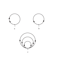
FIG. 1.: A particle on a ring: (a) classical return paths, (b) time reversed return paths, (c) time reversed return paths of different sizes.

Now let us analyze the effect of interaction. The expression for the return probability $W_{1}$ turns out to be insensitive to interaction due to exactly the same reason as in our first example: this probability is determined by the pairs of equivalent paths $q_{1}=q_{2}$ with $F\equiv 1$. In contrast to $W_{1}$, the return probability $W_{2}$ determined by the pairs of time reversed paths is affected by interaction. We will restrict ourselves to the most interesting physical situation when the energy of a particle $q$ remains conserved during its motion. Then the simplest pair of the time reversed paths is: $q_{-}(t^{\prime})=2R\sin(2\pi t^{\prime}/t)$ and $q_{+}(t^{\prime})$ is an even function of $t^{\prime}$. Substituting these paths into (11,12) after a simple integration we find

$$S_{R}=0,\;\;\;\;\;S_{I}(t)=\frac{2R^{2}C^{2}}{\omega}\coth\left(\frac{\omega}{2T}\right)\left(\frac{t}{2\pi}\right)^{2}\frac{\sin^{2}(\omega t/2)}{(1-\omega^{2}t^{2}/4\pi^{2})^{2}},$$ (24)

The result (24) demonstrates that the return probability $W_{2}$ for a particle $q$ after a time $t$ for the time reversed paths acquires the factor

$$F=\exp(-S_{I}(t)),$$ (25)

due to interaction with a harmonic oscillator with a frequency $\omega$. The probability $W_{1}$ remains unaffected.

The whole consideration can be trivially generalized to the case of more complicated time reversed paths with an arbitrary winding numbers $m$. In this case we again find an additional factor (25) in the interference term $W_{2}$ and $S_{I}$ is determined by an expression similar to (24) which also depends on $m$. The term $S_{R}$ is again zero for such paths for all $m$. Since no new effects emerge at $m>1$, in what follows we will analyze only the simplest case $m=1$ (24).

The first conclusion one can draw from the result (24) is that no qualitative changes in the system behavior emerges if one varies the temperature $T$. The value $S_{I}(t)$ is smaller at low $T\ll\omega$ as compared to the high temperature limit $T\gg\omega$ but the effect persists even at $T=0$. Thus the relation between $T$ and $\omega$ turns out to be important only in a quantitative sense, no qualitative dependence on this relation should be expected.

A much more important parameter is $\omega t$. We see that the value $S_{I}(t)$ and hence $W_{2}$ oscillate in time with a period $2\pi/\omega$. After each such period the interference term $W_{2}$ restores its “nonineracting” value while at all intermediate times the value $W_{2}$ is smaller than in the noninteracting case. In this situation we still cannot speak about decoherence: the system keeps information about its initial phase and periodically returns to its initial state. On top of that if the radius of the ring $R$ is constant in time (see below) we have $S_{I}\propto 1/t^{2}$, i.e. the oscillations of $W_{2}$ practically disappear in the long time limit. All these results are not surprizing: one should not expect to find the decoherence effect in the system of two quantum mechanical particles.

Quantum decoherence appears after the next step: we again modify our model coming from the interaction with one oscillator to the infinite set of oscillators with the ohmic spectrum (14). In this case after the integration of (24) over $\omega$ one gets

$$S_{I}=\frac{\eta R^{2}}{\pi}\int zdz\frac{\sin^{2}(\pi z)}{(1-z^{2})^{2}}\coth\left(\frac{\pi z}{Tt}\right).$$ (26)

This equation yields $S_{I}\sim\eta R^{2}$ at $T=0$ and $S_{I}\sim\eta TR^{2}t$ at $Tt\gg 1$. These results are in a nice qualitative agreement with those obtained in the exactly solvable model studied above. There the exponential decay of the off-diagonal elements of the initial density matrix $\rho(q_{-i})\propto\exp(-t/\tau_{0})$ with $\tau_{0}\sim 1/\eta Tq_{-i}^{2}$ was found at any $T>0$ while at $T=0$ a power law decay (21) was observed. In both cases the similarity is obvious if one interchanges $R$ and $q_{-i}$.

We observe from (25) that if $S_{I}$ is small the influence functional $F\simeq 1$ and no decoherence occurs. However for $S_{I}\gg 1$ the interference of the time-reversed paths is completely suppressed, and quantum dephasing takes place. By setting $S_{I}\sim 1$ we can, therefore, define the typical size of the ring $R\sim L_{\varphi}$ beyond which the effect of quantum decoherence becomes important. In our particular example the characteristic dephasing length $L_{\varphi}$ decreases as $1/t$ at $Tt\gg 1$ and it is constant

$$L_{\varphi}\sim 1/\sqrt{\eta}$$ (27)

at $T=0$. This is the effect of quantum decoherence.

Note that by fixing $R$ and increasing $t$ in our problem we effectively decrease the particle velocity $v_{0}=2\pi R/t$ which is eventually sent to zero as $t$ approaches infinity. Therefore it is quite natural that at $T=0$ the interference term $W_{2}$, although suppressed by a factor $F=\exp(-S_{I})$, does not decay in time. Qualitatively the same property is observed in our result for the decoherence time in a disordered metal (1): if we treat $v_{F}$ as a formal parameter which may be put equal to zero we will immediately arrive at a zero decoherence rate $1/\tau_{\varphi}$ in this limit. The same is true for the high temperature result [12, 13, 14, 15].

The above situation is, however, not very relevant for a metal where conducting electrons move with the velocity $v_{0}\simeq v_{F}$ which absolute value does not change in time. Thus to account for that we should rather keep the velocity of a particle $v_{0}$ fixed. This implies that as we increase $t$ the radius $R$ for a classical return path increases linearly with time. In other words, we can slightly modify our model allowing our particle to choose the ring with a proper $R$ for each time $t$ (see Fig. 1c). Then we immediately observe that $S_{I}$ (26) grows in time as $S_{I}\propto t^{2}$ at $T=0$ and $S_{I}\propto t^{3}$ at $Tt\gg 1$, i.e. in this case the decay of the quantum interference term $W_{2}$ caused by interaction with the Caldeira-Leggett bath of oscillators is faster than exponential. Finally, let us note that in a disordered metal, although the length of the electron trajectory increases linearly with time, the dynamics is diffusive and the effective loop size grows as $R^{2}\sim Dt$. Substituting this expression into (26) one obtains

$$F=\left\{\begin{array}[]{ll}\exp(-t/\tau_{\varphi}),\;\;\;\;\;\tau_{\varphi}=a/D\eta,&Tt\ll 1\\ \exp(-(t/\tau_{\varphi})^{2}),\;\;\;\;\tau_{\varphi}=b(D\eta T)^{-1/2},&Tt\gg 1\end{array}\right.$$ (28)

where $a$ and $b$ are unimportant numerical coefficients of order one.

Although the above simple model cannot be directly applied to disordered metals it demonstrates several important properties which will be also observed in a rigorous calculation. One such property is that the suppression of quantum interference between time reversed paths increases if the size of the loop grows in time. Another property is that oscillators with $\omega\gg T$ may give the dominating contribution to dephasing. In the above model the frequencies $\omega\sim 1/t$ give the maximum contribution, but if the spectrum of the problem is different (as e.g. in a disordered metal, see below) high frequency modes $\sim\omega_{c}$ may also become important. The physical reasons for this conclusion were already clarified above: in order to have energy exchange in an interacting system it is not necessary to excite the high frequency oscillators, broadening of their ground state levels is sufficient. It is well known that the high frequency cutoff $\omega_{c}$ enters the expression for the interaction induced decoherence rate of a quantum particle in the periodic [8, 9] and the double well potentials [10]. The same is observed here for an exactly solvable model of a free damped particle in the limit $T=0$.

Our model also demonstrates at which step of our calculation the effect of dephasing appears. Interaction of the particle $q$ with one harmonic oscillator leads to the oscillations of the interference term $W_{2}$ with the oscillator frequency $\omega$. These oscillations are natural since the initial state is not the eigenstate of the system. Yet no dephasing appears. If coupling to many oscillators with different frequencies is introduced the probability $W_{2}$ will be always suppressed and the system will never return to its initial state. Obviously this mechanism of dephasing has nothing to do with the temperature of the environment and it persists even at $T=0$. In this limit the exponential decay of $W_{2}$ in time is due to increase of the loop size with $t$. The phase breaking length $L_{\varphi}$ (27) depends only on the interaction strength and appears to be (roughly) insensitive to the particular (e.g. ballistic or diffusive) type of a particle motion.

D Scattering problem and perturbation theory

One might wonder what is the relation between the above analysis and the standard perturbative treatment of a scattering problem for a quantum particle interacting with a harmonic oscillator. Beside its general importance the scattering approach is also of a practical relevance because it is frequently applied to conductance calculations in mesoscopic systems.

The usual definition of a scattering problem operates with in- and out-scattering states measured after exactly infinite time. In other words, the limit $t\to\infty$ is taken already at the very first step, and the whole calculation is carried out only in this limit. This is sufficient in many physical situations, but not for our problem due to the reasons to be clarified below. Here we will keep $t$ finite (although possibly large) throughout the calculation and let it go to infinity in the end. With this in mind a direct connection to the scattering problem can be easily established.

Consider a quantum particle $q$ scattered on a harmonic oscillator with a frequency $\omega$. Before scattering the oscillator is assumed to be in its ground state, and the particle is in the state with wave function $\psi_{i}$ and the energy $E_{i}$. Assuming the interaction to be of the same form as in (9) and proceeding perturbatively in the interaction strength $C$ one can easily derive the probability $W(t)$ for a particle $q$ to leave the state $\psi_{i}$ after the time $t$. It is just the sum of the transition probabilities $W_{if}$ into all possible final states $\psi_{f}$ which are orthogonal to $\psi_{i}$ in the absence of interaction. One easily finds (see e.g. [4])

$$W=\sum_{f\neq i}W_{if}=2\sum_{f\neq i}|\langle i|Cq|f\rangle|^{2}\frac{\sin^{2}(\Delta E_{if}t/2)}{\omega(\Delta E_{if})^{2}},$$ (29)

where $\Delta E_{if}=\omega+E_{f}-E_{i}$. This result implies $dW/dt\propto\sin(\Delta E_{if}t)/\Delta E_{if}$, i.e. at large $t$ the transition rate experiences fast oscillations and approaches $\delta(\Delta E_{if})$ at $t\to\infty$. If $E_{f}>E_{i}$ for all $f$ (i.e. $\psi_{i}$ describes the ground state of the noninteracting problem) the transitions are highly improbable at sufficiently long times and one may conclude that with the dominating probability the particle remains in its initial state and no quantum dephasing takes place. We would like to emphasize, however, that the time average of the escape probability $W$ (29) is not equal to zero already in this case. This is a direct consequence of the energy-time uncertainty principle.

Let us now consider scattering on many oscillators. As before we will assume that the frequency spectrum for these oscillators is ohmic (14). In order to define the scattering problem we also assume that interaction exists only in a certain space region $-q_{0}/2<q<q_{0}/2$, i.e. we put $C=C_{0}(\Theta(q+q_{0}/2)-\Theta(q-q_{0}/2))$. Without interaction the eigenstates of a problem are the plane waves $\psi_{i/f}(q,t)=(L)^{-1/2}\exp(ip_{i/f}q-iE_{i/f}t)$ where $E_{i/f}=p_{i/f}^{2}/2m$. The transition matrix elements can be easily evaluated. They give an important contribution for $|p_{f}-p_{i}|q_{0}<1$ in which case we get $\langle i|Cq|f\rangle|^{2}\sim C_{0}^{2}q_{0}^{6}(p_{f}-p_{i})^{2}/L^{2}$. Subsituting this expression into (29) and carrying out the summation over the final states $\sum_{f}\to L\int dp_{f}$ and over the oscillator frequencies (making use of (15) with $C\to C_{0}$), we find

$$W(t)\sim\frac{\eta q_{0}^{6}}{L}\int_{0}^{\omega_{c}}\omega d\omega\int_{-1/q_{0}}^{1/q_{0}}dp_{f}(p_{f}-p_{i})^{2}\frac{\sin^{2}(\Delta E_{if}t/2)}{(\Delta E_{if})^{2}}.$$ (30)

Further assuming that the initial particle energy is small $E_{i}\to 0$ after simple integrations we obtain

$$W(t)\sim\frac{\eta q_{0}^{3}}{L}\ln(\omega_{c}\mbox{min}(t,mq_{0}^{2})).$$ (31)

We observe that the escape probability $W(t)$ is not zero and, moreover, it is not necessarily small. The reason for that is transparent. Although the contribution of each oscillator to $W(t)$ is small, it is not zero at any finite $t$ due to the energy-time uncertainty principle. The sum of these small contributions from many oscillators is finite and yields the result (31). We would like to emphasize that by no means this result is in contradiction with the energy conservation law, rather it demonstrates that one should be careful applying the energy arguments to describe the time evolution of an interacting quantum system, especially if it consists of an infinite number of degrees of freedom. Even at times much larger than the characteristic time scale (in our problem the relevant time scale is set by the dephasing time $\tau_{\varphi}$) the energy uncertainty may be sufficient for $W(t)$ to significantly differ from zero.

In order to observe the relation of a perturbative expression (31) to our previous results we set $q_{0}$ to be of order of the system size $q_{0}\sim L$. After that the similarity between (31) and e.g. eqs. (21,26) becomes completely obvious. Requiring that $W(t,L)\sim 1$ (the escape is complete) and using (31) with $q_{0}\sim L$ one immediately arrives at the estimate (27) for the decoherence length $L_{\varphi}\sim 1/\sqrt{\eta}$ derived previously with the quasiclassical analysis of the exact influence functional. This result leaves no room for doubts concerning the validity of the quasiclassical description of quantum dephasing at $T=0$. In fact, the comparison of the results (21,31) with (26) demonstrates that the quasiclassical approximation rather underestimates the dephasing effect of interaction: $L_{\varphi}$ may only become shorter if fluctuations around the classical trajectory are taken into account.

Another obvious conclusion is that at any $T$ (including $T=0$) the effect of quantum decoherence in not only due to low frequency oscillators which, moreover, can be even completely unimportant. The relative contribution of oscillators with small $\omega$ depends on the particular form of the spectrum ($\sim\omega^{\gamma}$), being more important in the subohmic case $\gamma<1$ and practically irrelevant in the superohmic case $\gamma>1$ when the high frequency oscillators yield the main effect. The latter situation will be encountered in the next section where it will be shown that for a $d$-dimensional disordered metal one has $\gamma=1+d/2$. Again we emphasize that the above results do not imply that the processes with high energy transfers are important for dephasing at any $T$. It is erroneous to interpret the parameter $\omega$ as describing the energy transfer: in our calculation the integral over $\omega$ always represents the summation over the bath oscillators (cf. eqs. (14-15)). No high frequency oscillators need to be excited, (small) energy uncertainty for infinitely many oscillators is sufficient to provide (large) dephasing for a particle $q$.

III Quantum Decoherence in a Disordered Metal

In order to provide a quantitative description of the effect of quantum decoherence in disordered metals it is necessary to go beyond the simple model considered in the previous section and account for $(a)$ Fermi statistics and the Pauli principle, $(b)$ the specifics of Coulomb interaction in a $d$-dimensional system and $(c)$ the effect of disorder. The corresponding analysis is presented below.

A Density matrix and effective action

Our starting point is the standard Hamiltonian for electrons in a disordered metal $H_{\rm el}=H_{0}+H_{\rm int}$, where

$$H_{0}=\int{\rm d}{\bf r}\psi^{+}_{\sigma}({\bf r})\left[-\frac{\nabla^{2}}{2m}-\mu+U({\bf r})\right]\psi_{\sigma}({\bf r}),$$ (32)

$$H_{int}=\frac{1}{2}\int{\rm d}{\bf r}\int{\rm d}{\bf r^{\prime}}\psi^{+}_{\sigma}({\bf r})\psi^{+}_{\sigma^{\prime}}({\bf r^{\prime}})e^{2}v({\bf r}-{\bf r^{\prime}})\psi_{\sigma^{\prime}}({\bf r^{\prime}})\psi_{\sigma}({\bf r}).$$ (33)

Here $\mu$ is the chemical potential, $U({\bf r})$ accounts for a random potential due to nonmagnetic impurities, and $v({\bf r})=1/|{\bf r}|$ represents the Coulomb interaction between electrons.

Let us define the electron Green-Keldysh function [16]

$$\hat{G}\equiv\left(\begin{array}[]{cc}G_{11}&-G_{12}\\ G_{21}&-G_{22}\end{array}\right)=\frac{\int{\rm D}V_{1}{\rm D}V_{2}\;\hat{G}_{V}\;e^{{\rm i}S[V_{1},V_{2}]}}{\int{\rm D}V_{1}{\rm D}V_{2}\;e^{{\rm i}S[V_{1},V_{2}]}},$$ (34)

where

$${\rm i}S[V_{1},V_{2}]=2{\rm Tr}\ln\hat{G}_{V}^{-1}+{\rm i}\int\limits_{0}^{t}{\rm d}t^{\prime}\int{\rm d}{\bf r}\frac{(\nabla V_{1})^{2}-(\nabla V_{2})^{2}}{8\pi}.$$ (35)

Here we performed a standard Hubbard-Stratonovich transformation introducing the path integral over a scalar potential field $V$ in order to decouple the $\psi^{4}$-interaction in (33). In (34,35) we explicitely defined the fields $V_{1}(t)$ and $V_{2}(t)$ equal to $V(t)$ respectively on the forward and backward parts on the Keldysh contour [16].

The matrix function $\hat{G}_{V}$ obeys the equation

$$\left({\rm i}\frac{\partial}{\partial t_{1}}-\hat{H}_{0}({\bf r}_{1})+e\hat{V}(t_{1},{\bf r}_{1})\right)\hat{G}_{V}=\delta(t_{1}-t_{2})\delta({\bf r}_{1}-{\bf r}_{2});$$ (36)

where

$$\hat{H}_{0}=H_{0}\hat{1}=\left(\begin{array}[]{c}\frac{-\nabla^{2}}{2m}-\mu+U({\bf r})\qquad 0\\ 0\qquad\frac{-\nabla^{2}}{2m}-\mu+U({\bf r})\end{array}\right);\;\;\;\;\;\;\;\hat{V}=\left(\begin{array}[]{cc}V_{1}(t,{\bf r})&0\\ 0&V_{2}(t,{\bf r})\end{array}\right).$$ (37)

The solution of (36) is fixed by the Dyson equation

$$\hat{G}_{V}(t_{1},t_{2})=\hat{G}_{0}(t_{1},t_{2})-\int\limits_{0}^{t}{\rm d}t^{\prime}\hat{G}_{0}(t_{1},t^{\prime})e\hat{V}(t^{\prime})\hat{G}_{V}(t^{\prime},t_{2}).$$ (38)

The matrix $\hat{G}_{0}$ is the electron Green-Keldysh function without the field $V$.

It is well known that the 1,2-component of the Green-Keldysh matrix ${\bf\hat{G}}$ is directly related to the exact electron density matrix

$$\rho(t;{\bf r},{\bf r^{\prime}})=-{\rm i}G_{12}(t,t;{\bf r},{\bf r^{\prime}})=\langle\rho_{V}(t;{\bf r},{\bf r^{\prime}}\rangle_{V_{1},V_{2}},$$ (39)

where we also defined the “density matrix” $\rho_{V}(t)$ related to the 1,2-component of the matrix $\hat{G}_{V}$ and performed the average over the fields $V_{1}$ and $V_{2}$ as defined in (34). The density matrix $\rho$ contains all necessary information about the system dynamics in the presence of interaction.

Making use of eqs. (36-38) after some formal manipulations (see [2] for details) one arrives at the equation describing the time evolution of the density matrix:

$${\rm i}\frac{\partial\rho_{V}}{\partial t}=[H_{0}-eV^{+},\rho_{V}]-(1-\rho_{V})\frac{eV^{-}}{2}\rho_{V}-\rho_{V}\frac{eV^{-}}{2}(1-\rho_{V}),$$ (40)

where we defined $V^{+}=(V_{1}+V_{2})/2$ and $V^{-}=V_{1}-V_{2}$. It is important to emphasize that the derivation of this equation was performed without any approximation, i.e. the result (40) is exact. The equation (40) fully accounts for the Pauli principle which is important for the fluctuations of the field $V^{-}$. This field is irrelevant for dephasing. It is quite obvious from (40) that the field $V^{+}(t,{\bf r})$ plays the same role as an external field. All electrons move collectively in this field, its presence is equivalent to local fluctuations of the Fermi energy $\mu\to\mu+eV^{+}(t,{\bf r})$. The Pauli principle does not play any role here. There is no way how the density matrix $\rho$ can “distinguish” the intrinsic fluctuating field $V^{+}$ from the stochastic external field, be it classical or quantum. Since the external field is known to lead to dephasing of the wave function, the field $V^{+}$ should produce the same effect. As the equation (40) is exact this conclusion is general and does not depend on approximations.

In order to proceed further let us assume Coulomb interaction to be sufficiently weak and expand the action (35) in powers of $V$ up to terms proportional to $V^{2}$. After a straightforward calculation (see e.g. [2]) one finds

$${\rm i}S[V_{1},V_{2}]={\rm i}\int\frac{{\rm d}\omega{\rm d}^{3}k}{(2\pi)^{4}}V^{-}(-\omega,-k)\frac{k^{2}\epsilon(\omega,k)}{4\pi}V^{+}(\omega,k)-$$ (41)

$$-\frac{1}{2}\int\frac{{\rm d}\omega{\rm d}^{3}k}{(2\pi)^{4}}V^{-}(-\omega,-k)\frac{k^{2}{\rm Im}\epsilon(\omega,k)}{4\pi}\coth\left(\frac{\omega}{2T}\right)V^{-}(\omega,k);$$ (42)

where $\epsilon(\omega,k)$ is the dielectric susceptibility of a disordered metal

$$\epsilon(\omega,k)=1+\frac{4\pi\sigma}{-{\rm i}\omega+Dk^{2}}.$$ (43)

Here $\sigma=2e^{2}N_{0}D$ is the classical Drude conductivity, $N_{0}$ is the metallic density of states and $D=v_{F}l/3$ is the diffusion coefficient. For the sake of simplicity in eq. (43) we disregarded the phonon contribution which will not be important for us here. The expression (43) is valid for small wave vectors $k<1/l$ and small frequencies $\omega<1/\tau_{e}=v_{F}/l$.

Note, that if one considers only nearly uniform in space ($k\approx 0$) fluctuations of the field $V$ one immediately observes that eqs. (42,43) exactly coincide with the real time version of the Caldeira-Leggett action [5, 6, 8] in this limit (cf. (10-12,15)). Taking into account only uniform fluctuations of the electric field one can also derive the Caldeira-Leggett action expressed in terms of the electron coordinate only. In this case the effective viscosity $\eta$ in the Caldeira-Leggett influence functional is $\eta\sim e^{2}R_{s}$, where $R_{s}$ is the sample resistance (in contrast to the effective viscosity for the field $V$ which is proportional to $1/R_{s}$).

For our present purposes it is not sufficient to restrict ourselves to uniform fluctuations of the collective coordinate $V$ of the electron environment. The task at hand is to evaluate the kernel of the operator

$$J=\sum_{V}U|V\rangle\langle V|U^{+}$$

where the sum runs over the states of the electromagnetic environment with all possible $k$ and $\omega$. Averaging over $V^{+},V^{-}$ amounts to calculating Gaussian path integrals with the action (42) and can be easily performed. We obtain

$$J(t,t^{\prime};{\bf r}_{1f},{\bf r}_{2f};{\bf r}_{1i},{\bf r}_{2i})=\int\limits_{{\bf r}_{1}(t^{\prime})={\bf r}_{1i}}^{{\bf r}_{1}(t)={\bf r}_{1f}}{\rm D}{\bf r}_{1}\int\limits_{{\bf r}_{2}(t^{\prime})={\bf r}_{2i}}^{{\bf r}_{2}(t)={\bf r}_{2f}}{\rm D}{\bf r}_{2}\int{\rm D}{\bf p}_{1}{\rm D}{\bf p}_{2}\times$$

$$\times\exp\big{\{}{\rm i}S_{0}[{\bf r}_{1},{\bf p}_{1}]-{\rm i}S_{0}[{\bf r}_{2},{\bf p}_{2}]-{\rm i}S_{R}[{\bf r}_{1},{\bf p}_{1},{\bf r}_{2},{\bf p}_{2}]-S_{I}[{\bf r}_{1},{\bf r}_{2}]\big{\}};$$ (44)

where

$$S_{0}[{\bf r},{\bf p}]=\int\limits_{t^{\prime}}^{t}{\rm d}t^{\prime\prime}\bigg{(}{\bf p\dot{r}}-\frac{{\bf p}^{2}}{2m}-U({\bf r})\bigg{)}$$ (45)

is the electron action,

$$S_{R}[{\bf r}_{1},{\bf p}_{1},{\bf r}_{2},{\bf p}_{2}] = \frac{e^{2}}{2}\int\limits_{t^{\prime}}^{t}{\rm d}t_{1}\int\limits_{t^{\prime}}^{t}{\rm d}t_{2}\big{\{}R(t_{1}-t_{2},{\bf r}_{1}(t_{1})-{\bf r}_{1}(t_{2}))\big{[}1-2n\big{(}{\bf p}_{1}(t_{2}),{\bf r}_{1}(t_{2})\big{)}\big{]}-$$ (49)

$$-R(t_{1}-t_{2},{\bf r}_{2}(t_{1})-{\bf r}_{2}(t_{2}))\big{[}1-2n\big{(}{\bf p}_{2}(t_{2}),{\bf r}_{2}(t_{2})\big{)}\big{]}$$

$$+R(t_{1}-t_{2},{\bf r}_{1}(t_{1})-{\bf r}_{2}(t_{2}))\big{[}1-2n\big{(}{\bf p}_{2}(t_{2}),{\bf r}_{2}(t_{2})\big{)}\big{]}-$$

$$-R(t_{1}-t_{2},{\bf r}_{2}(t_{1})-{\bf r}_{1}(t_{2}))\big{[}1-2n\big{(}{\bf p}_{1}(t_{2}),{\bf r}_{1}(t_{2})\big{)}\big{]}\big{\}},$$

where $n({\bf p},{\bf r})$ is the occupation number and

$$S_{I}[{\bf r}_{1},{\bf r}_{2}] = \frac{e^{2}}{2}\int\limits_{t^{\prime}}^{t}{\rm d}t_{1}\int\limits_{t^{\prime}}^{t}{\rm d}t_{2}\bigg{\{}I(t_{1}-t_{2},{\bf r}_{1}(t_{1})-{\bf r}_{1}(t_{2}))+I(t_{1}-t_{2},{\bf r}_{2}(t_{1})-{\bf r}_{2}(t_{2}))-$$ (51)

$$-I(t_{1}-t_{2},{\bf r}_{1}(t_{1})-{\bf r}_{2}(t_{2}))-I(t_{1}-t_{2},{\bf r}_{2}(t_{1})-{\bf r}_{1}(t_{2}))\bigg{\}}.$$

In equilibrim $n$ is just the Fermi function. In this case at the scales $|{\bf r}|>l$ the functions $R$ and $I$ are defined by the equations

$$R(t,{\bf r}) = \int\frac{{\rm d}\omega{\rm d}^{3}k}{(2\pi)^{4}}\vskip 6.0pt plus 2.0pt minus 2.0pt\frac{4\pi}{k^{2}\epsilon(\omega,k)}e^{-i\omega t+i{\bf kr}}$$ (52)

$$I(t,{\bf r}) = \int\frac{{\rm d}\omega{\rm d}^{3}k}{(2\pi)^{4}}\vskip 6.0pt plus 2.0pt minus 2.0pt{\rm Im}\left(\frac{-4\pi}{k^{2}\epsilon(\omega,k)}\right)\coth\bigg{(}\frac{\omega}{2T}\bigg{)}e^{-i\omega t+i{\bf kr}}.$$ (53)

The expression in the exponent of eq. (44) defines the real time effective action of the electron propagating in a disordered metal and interacting with other electrons. The first two terms represent the electron action $S_{0}$ (45) on two branches of the Keldysh contour while the last two terms $S_{R}$ and $S_{I}$ determine the influence functional (cf. eqs. (5,10-12,15)) of the effective electron environment. As can be seen from eqs. (49-53) this influence functional is not identical to one derived in the Caldeira-Leggett model. However on a qualitative level the similarity is obvious: in both models the influence functionals describe the effect of a certain effective dissipative environment.

B Decoherence time

Let us first neglect the terms $S_{R}$ and $S_{I}$ describing the effect of Coulomb interaction. Then in the quasiclassical limit $p_{F}l\gg 1$ the path integral (44) is dominated by the saddle point trajectories for the action $S_{0}$:

$${\bf\dot{p}}=-\partial H_{0}/\partial{\bf r},\quad{\bf\dot{r}}=\partial H_{0}/\partial{\bf p}$$ (54)

with obvious boundary conditions ${\bf r}_{1}(t^{\prime})={\bf r}_{1i}$, ${\bf r}(t)={\bf r}_{1f}$ for the action $S_{0}[{\bf r}_{1},{\bf p}_{1}]$ and ${\bf r}_{2}(t^{\prime})={\bf r}_{2i}$, ${\bf r}_{2}(t)={\bf r}_{2f}$ for the action $S_{0}[{\bf r}_{2},{\bf p}_{2}]$.

Since in a random potential $U({\bf r})$ there is in general no correlation between different classical paths ${\bf r}_{1}(t)$ and ${\bf r}_{2}(t)$ these paths give no contribution to the integral (44): the difference of two actions $S_{0}$ in the exponent may have an arbitrary value and the result averages out after summation. Thus only the paths with $S_{0}[{\bf r}_{1},{\bf p}_{1}]\simeq S_{0}[{\bf r}_{2},{\bf p}_{2}]$ provide a nonzero contribution to the path integral (44). Two different classes of paths can be distinguished (see e.g. [13]):

i) The two classical paths are almost the same: ${\bf r}_{1}(t^{\prime\prime})\simeq{\bf r}_{2}(t^{\prime\prime})$, ${\bf p}_{1}(t^{\prime\prime})\simeq{\bf p}_{2}(t^{\prime\prime})$ (cf. Fig. 1a). For such pairs we obviously have ${\bf r}_{1i}\simeq{\bf r}_{2i}$ and ${\bf r}_{1f}\simeq{\bf r}_{2f}$. Physically this corresponds to the picture of electrons propagating as nearly classical particles. In the diffusive limit these paths give rize to diffusons (see e.g. [12]) and yield the standard Drude conductance.

ii) The pairs of time reversed paths. In this case ${\bf r}_{1i}\simeq{\bf r}_{2f}$, ${\bf r}_{1f}\simeq{\bf r}_{2i}$ (cf. Fig. 1b,c). In the path integral (5) the trajectories ${\bf r}_{1}$ and ${\bf r}_{2}$ are related as ${\bf r}_{2}(t^{\prime\prime})\simeq{\bf r}_{1}(t+t^{\prime}-t^{\prime\prime})$ and ${\bf p}_{2}(t^{\prime\prime})\simeq-{\bf p}_{1}(t+t^{\prime}-t^{\prime\prime})$. In a disordered metal these paths correspond to Cooperons and give rize to the weak localization correction to conductivity $\delta\sigma_{d}$. This correction is expressed in terms of the time integrated probability $W(t)$ for all diffusive paths to return to the same point after the time $t$ (see e.g. [12, 13]). In the absence of any kind of interaction which breaks the time reversal symmetry this value coincides with the classical return probability and is given by the formula $W_{0}(t)=(4\pi Dt)^{-d/2}a^{-(3-d)}$, where $d$ is the system dimension and $a$ is the transversal sample size.

The weak localization correction $\delta\sigma_{d}$ diverges for $d\leq 2$. This divergence can be cured by introducing the upper limit cutoff at a certain time $\tau_{\varphi}$. This time is usually reffered to as decoherence time. One finds [12, 13]:

$$\delta\sigma_{d}=\left\{\begin{array}[]{ll}-\frac{e^{2}}{2\pi^{2}}\ln\left(\frac{\tau_{\varphi}}{\tau_{e}}\right),&d=2\\ -\frac{e^{2}}{\pi}\sqrt{D\tau_{\varphi}},&d=1.\end{array}\right.$$ (55)

The physical reason for the existence of a finite $\tau_{\varphi}$ is the electron-electron interaction which breaks the time reversal symmetry in our problem. To evaluate $\tau_{\varphi}$ we first note that the functions $R$ and $I$ (53) change slowly at distances of the order of the Fermi wavelength $1/p_{F}$. Therefore we may put ${\bf r}_{1}(t^{\prime\prime})={\bf r}(t^{\prime\prime})$, ${\bf r}_{2}(t^{\prime\prime})={\bf r}_{t}(t^{\prime\prime})\equiv{\bf r}(t+t^{\prime}-t^{\prime\prime})$. Here ${\bf r}(t^{\prime\prime})$ is a classical trajectory with the initial point ${\bf r}(t^{\prime})=0$ and the final point $|{\bf r}(t)|<l$, i.e. we consider trajectories which return to the vicinity of the initial point. The contribution from the time reversed paths $W_{2}$ to the return probability has the form

$$W_{2}(t-t^{\prime})\simeq W_{20}(t-t^{\prime})F,\;\;\;F=\left\langle e^{-{\rm i}S_{R}[t,t^{\prime};{\bf r},{\bf p};{\bf r}_{t},{\bf p}_{t}]-S_{I}[t,t^{\prime};{\bf r},{\bf r}_{t}]}\right\rangle_{r},$$ (56)

where $W_{20}$ is the probability without interaction and the average is taken over all diffusive paths returning to the initial point. The value $F$ in (56) decays exponentially in time, therefore we may put the average inside the exponent. It is easy to observe that the term $S_{R}$ gives no contribution to this average. Working out the average of $S_{I}$ we obtain

$$F=e^{-\left\langle S_{I}[t,0;{\bf r},{\bf r}_{t}]\right\rangle_{r}}=\exp\left(-te^{2}\int\limits_{-\infty}^{+\infty}{\rm d}t\langle I(t,{\bf r}(t)-{\bf r}(0))\rangle_{r}\right)$$ (57)

To find the average over the diffusive paths, we introduce the Fourier transform of the function $I(t,{\bf r})$ and replace $\langle e^{-ik({\bf r}(t)-{\bf r}(t^{\prime}))}\rangle_{r}$ by $e^{-Dk^{2}|t-t^{\prime}|}$. Then we get

$$\ln F(t)=-\frac{te^{2}}{a^{3-d}}\int\frac{{\rm d}\omega{\rm d}^{d}k}{(2\pi)^{d+1}}{\rm Im}\left(\frac{-4\pi}{k^{2}\epsilon(\omega,k)}\right)\coth\left(\frac{\omega}{2T}\right)\frac{Dk^{2}}{\omega^{2}+D^{2}k^{4}}$$ (58)

Let us first consider a quasi-one-dimensional system with $a\leq l$. Making use of eqs. (58,43) and integrating over $k$ we find

$$\ln F(t)=-t\frac{e^{2}\sqrt{2D}}{\sigma_{1}}\int\limits_{1/t}^{1/\tau_{e}}\frac{{\rm d}\omega}{2\pi}\frac{\coth(\omega/2T)}{\sqrt{\omega}}.$$ (59)

The upper cutoff in (59) is chosen at the scale $\sim 1/\tau_{e}$ because at higher $\omega$ the diffusion approximation becomes incorrect. From (59) we obtain

$$F=\left\{\begin{array}[]{ll}\exp(-t/\tau_{\varphi}),\;\;\;\;\;\tau_{\varphi}\simeq\pi(3/2)^{1/2}\sigma_{1}/e^{2}v_{F},&t\ll 1/T^{2}\tau_{e}\\ \exp(-(t/\tau_{\varphi})^{3/2}),\;\;\;\;\tau_{\varphi}\simeq 0.5(\pi\sigma_{1}/D^{1/2}T)^{2/3},&t\gg 1/T^{2}\tau_{e}\end{array}\right.$$ (60)

In the long time limit (which cannot be reached at $T\to 0$) the decay of $F$ is faster than exponential (cf. [15]). At sufficiently low $T<(\tau_{e}\tau_{\varphi})^{-1/2}$ this difference becomes important only at $t\gg\tau_{\varphi}$ where $F$ is already exponentially suppressed. For smaller $t$ the decay is exponential and the decoherence rate increases linearly with $T$. Defining the effective decoherence length $L_{\varphi}\simeq\sqrt{D\tau_{\varphi}}$, in the temperature interval $1/2\tau_{\varphi}(0)<T<(\tau_{e}\tau_{\varphi}(0))^{-1/2}$ one finds

$$\frac{1}{L_{\varphi}^{2}(T)}=\frac{1}{L_{\varphi}^{2}(0)}+2\sqrt{2}\frac{L_{\varphi}(0)e^{2}}{\pi D\sigma_{1}}T,$$ (61)

where $L_{\varphi}(0)$ is the dephasing length at $T=0$. At temperatures lower than $1/2\tau_{\varphi}(0)$ the decoherence time and length are almost temperature independent. With the aid of eqs. (55,60) it is also easy to find the weak localization correction $\delta\sigma_{1}$ to the Drude conductance. In the limit $T=0$ we obtain

$$\frac{\delta\sigma_{1}}{\sigma_{1}}=-\frac{e^{2}}{\pi\sigma_{1}}\sqrt{D\tau_{\varphi}}\approx-\frac{1}{p_{F}s^{1/2}},$$ (62)

i.e. $\delta\sigma_{1}\approx-\sigma_{1}/\sqrt{N_{\rm ch}}$, where $N_{\rm ch}\sim p_{F}^{2}s$ is the effective number of conducting channels in a 1d mesoscopic system and $\sigma_{d}=\sigma a^{3-d}$ is the Drude conductance of a $d$-dimensional sample. Thus for $N_{\rm ch}\gg 1$ the weak localization correction is parametrically smaller than the Drude conductance even at $T=0$.

For 2d and 3d systems the same analysis yields

$$\frac{1}{\tau_{\varphi}} = \frac{e^{2}}{4\pi\sigma_{2}\tau_{e}}[1+2T\tau_{e}\ln(T\tau_{\varphi})],\;\;\;\;\;\;\;\quad{\rm 2d},$$ (63)

$$\frac{1}{\tau_{\varphi}} = \frac{e^{2}}{3\pi^{2}\sigma\sqrt{2D}\tau_{e}^{3/2}}[1+6(T\tau_{e})^{3/2}],\;\quad{\rm 3d},$$ (64)

The influence functional $F$ decays exponentially $F=\exp(-t/\tau_{\varphi})$ except for the case of 2d systems at high $T$ where one has $\ln F\propto-t\ln t$. We observe that also in this case the difference from a purely exponential decay is not significant and can be ignored.

C Further remarks

The above formalism provides a rigorous description of the effect of quantum decoherence in disordered metals and allows to derive the decoherence rate $1/\tau_{\varphi}$ at low $T$ for various dimensions. The physical reasons for dephasing of electron wave functions remain the same as in the case of a particle interacting with the Caldeira-Leggett bath of oscillators. The corresponding discussion is presented in the previous section. Here we only add several comments.

It might be interesting to investigate the average kinetic energy of an electron in a disordered metal in the presence of interaction. At low $T$ it turns out to be temperature independent due to the same reason as for a quantum particle in the bath of oscillators, i.e. due to interaction. A naive calculation along the same lines as in Section 2 yields $\langle m{\bf\dot{r}^{2}}/2\rangle-\mu\sim 1/\tau_{\varphi}$ at $T=0$. A more accurate analysis is beyond the frames of the present paper. This result is just a manifestation of the well known fact: the distribution function $n({\bf p})$ of interacting electrons (not quasiparticles) is nonzero for any ${\bf p}$ even at $T=0$ [17].

An obvious consequence of our results is that the decoherence rate $1/\tau_{\varphi}$ exceeds temperature at sufficiently low $T$. Does this fact imply the breakdown of the Fermi liquid theory (FLT) hypothesis at such $T$? From a formal point of view the violation of the inequality $T\tau_{\varphi}>1$ is yet insufficient for such a conclusion (see also [18]), although it obviously does not support the FLT hypothesis either. It was demonstrated in Section 2 that a finite decoherence rate for a certain variable of interest has no direct relation to the lifetime of quasiparticles (the latter is infinite in the case of a free particle in the Caldeira-Leggett bath). In our calculation $\tau_{\varphi}$ determines the dephasing time for real electrons and not for the Landau quasiparticles. Our result implies that interacting electrons are “bad” particles since their wave functions dephase even at $T=0$. The possibility to construct “better behaving” quasiparticles remains questionable for disordered metals. Furthermore, even if such quasiparticles exist their properties are completely unknown. Therefore at this stage they can hardly be used for calculation of any physical quantity. An important advantage of our method is that it allows for a direct calculation of measurable quantities in terms of interacting electrons without appealing to the Fermi liquid hypothesis.

IV Discussion of Experiments

Our results for the decoherence time at low $T$ turn out to be in a remarkably good agreement with available experimental data obtained in various physical systems. In Ref. [2] we have already carried out a detailed comparison between our theory and the experimental results [1] obtained for 1d Au wires. The agreement within a numerical factor of order one was observed for all samples studied in [1]. Since both $\tau_{\varphi}$ and $L_{\varphi}$ are defined with such an accuracy no better agreement can be expected in principle.

Here we will present a comparison of our theory with two other experiments carried out with 2d electron gas in semiconductor structures. These systems are somewhat different from the metallic ones mainly because of much higher effective resistance. The parameters of the systems were chosen in a way to realize a quasi 1d conducting system with disorder. One such experiment was carried out by Pooke et al. [19] in narrow Si pinched accumulation layer MOSFETs. These authors studied samples with resistances ranging from 120 to 360 k$\Omega$ and observed a finite decoherence rate $1/\tau_{\varphi}$ at all temperatures. On a log-plot (not shown) clear signs of saturation at low $T$ are seen. The corresponding data for $L_{\varphi}$ [19] obtained for 3 samples are presented in Fig. 2 and in the Table 1 together with our theoretical predictions. Note, that the experimental value of $L_{\varphi}$ at $T=0$ was obtained by a linear extrapolation $1/L^{2}_{\varphi}(T)=1/L^{2}_{\varphi}(0)+BT$ of the experimental data [19].

Table 1

$V_{g}$, $V_{p}$, V	$L_{\varphi}^{\rm exp}(0)$, $\mu$m	$L_{\varphi}^{\rm theor}(0)$, $\mu$m	$B^{\rm exp}$, $\mu$m-2K-1	$B^{\rm theor}$, $\mu$m-2K-1
60, 0	1.24	0.78	5.45	3.8
60, -3	0.85	0.58	7.83	5.4
75, -6	0.66	0.53	6.65	6

FIG. 2.: The experimental data [19] (symbols) fitted to our theory (solid lines).

The agreement between theory and experiment is within a numerical factor of order one, i.e. again within the accuracy of the definition of $L_{\varphi}$. Adjusting this numerical factor we observe a perfect fit of the experimental data by our theoretical curves (see Fig. 2). As predicted (cf. eq. (61)) at sufficiently low $T$ the value $1/L_{\varphi}$ increases linearly with temperature.

Very recently new measurements of the dephasing time $\tau_{\varphi}$ in quasi 1d $\delta$-doped GaAs structures with few conducting channels were reported [20]. The typical effective resistance of the samples [20] was $6\div 30$ M$\Omega$, i.e. it was even higher than in Ref. [19], the length and the width of the wires were 500 $\mu$m and 0.05 $\mu$m respectively. Experimental results for 3 different values of the gate voltage $V_{g}$ [20] are presented in the Table 2 together with our theoretical predictions. Again a perfect agreement between the maximum measured value $L_{\varphi}$ and the one derived from our theory is found for all $V_{g}$.

Table 2

$V_{g}$, V	$n$, $10^{12}$ cm-2	$R$, M$\Omega$	$L_{\varphi}^{\rm exp}$, $\mu$m	$L_{\varphi}^{\rm theor}(0)$, $\mu$m
+0.7	4	5.94	0.35	0.23
0	2.7	$\simeq$ 18	0.09	0.08
-0.35	2	$\simeq$ 36	0.06	0.04

The temperature dependence of the data $L_{\varphi}$ [20] is also in excellent agreement with our predictions at all $T$, see Fig. 3.

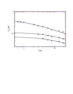
FIG. 3.: The experimental data [20] (symbols) fitted to our theory (solid lines).

In Ref. [20] the measured maximum values for $\tau_{\varphi}$ were compared with the theoretical formula suggested in Refs. [1, 21] and a discrepancy by a factor of 50 was reported. This fact allowed the authors to conclude [20] that their experimental results for $\tau_{\varphi}$ argue against the idea of decoherence by zero-point fluctuations of the electrons. The comparison of the data [20] with our theoretical results clearly demonstrates that this conclusion is simply an artefact of the inadequate choice of a theoretical formula adopted in [20]. The measurements of the decoherence rate [20] strongly support the idea of decoherence due to intrinsic quantum noise rather than argue against it.

In Ref. [20] also another interesting experimental observation was made: a crossover to a highly resistive state was found around $T\sim 1$ K. This observation was interpreted in [20] as a Thouless crossover to the regime of strong localization and was also qualified as contradicting the very idea of quantum decoherence at $T=0$. Several comments are in order.

(i) For the systems studied in [20] one has $\sqrt{N_{\rm ch}}\sim 2\div 3$. Hence, the weak localization correction at low $T$ (62) should be of the same order as the Drude conductance (in fact, this is exactly what was observed in [20]) and the Thouless crossover cannot be ruled out theoretically for such small $N_{\rm ch}$. Also the result for $\tau_{\varphi}$ may become more complicated for small $N_{\rm ch}$ [2] because of a somewhat more important role of capacitive effects. This may in principle lead to a relative increase of $L_{\varphi}$ (it appears, however, that this effect is not very important in [20]). Thus even the presence of a Thouless crossover in the samples [20] would by no means contradict our theoretical results and hence the idea of quantum decoherence at $T=0$.

(ii) The interpretation of the observed effect as a Thouless crossover is not quite convincing. This interpretation is based on two reasons [20]: (i) at the crossover $L_{\varphi}$ was found to be “only” $\sim 3$ times smaller than $l_{\rm loc}$ and (ii) the resistance of a wire segment of the length $\sim l_{\rm loc}$ was found to be $\sim 20$ k$\Omega$. The first observation does not contradict to our theory which predicts $l_{\rm loc}/L_{\varphi}\sim\sqrt{N_{\rm ch}}\sim 3$ at low $T$. As to the resistance of a segment $\sim l_{\rm loc}$ it is of the order of the quantum resistance unit also at temperatures $T\sim 3\div 10$K, i.e. well above the crossover. Hence, no definite conclusion can be drawn.

(iii) The expression for $l_{loc}$ used in [20] makes sense only provided the condition $L_{\varphi}>L\gg l_{loc}$ is satisfied ($L$ is the wire length). For $L_{\varphi}\ll L$ the wire can be viewed as $N\sim L/L_{\varphi}$ independent samples connected in series (in [20] $N$ is typically of order $10^{3}\div 10^{4}$). Since the the length of each of such samples $L_{\varphi}$ is $\sim 3$ times smaller than the localization length $l_{loc}$ it is somewhat naive to seriously believe that strong localization can be observed in such samples relying only on the “order-of-magnitude” character of the relation between $L_{\varphi}$ and $l_{loc}$ at the crossover. Moreover, assuming the dependence $L_{\varphi}\propto T^{-1/3}$ one immediately observes that the “standard” crossover condition $l_{\rm loc}\sim L_{\varphi}$ would hold at temperatures $\sim 30$ times smaller than the actual crossover temperature, i.e. at $T\sim 20\div 30$ mK. We see no way how the Thouless crossover can be expected above this temperature range for the systems studied in [20].

(iv) The inequality $T\tau_{\varphi}\gg 1$ is violated in [20] at all relevant $T$: at the crossover one has $T\tau_{\varphi}\sim 0.3\div 0.5$ depending on the sample, and $T\tau_{\varphi}$ remains of order one even at $T\sim 10\div 20$K, i.e. well in the weak localization regime. If one believes that the violation of the above condition signals the breakdown of FLT due to interaction the whole discussion of the Thouless crossover becomes pointless. An alternative would be to acknowledge that the value $T\tau_{\varphi}$ may not be the relevant parameter as far as FLT is concerned. But in any case real electrons dephase and therefore can hardly be described within the Thouless scenario of strong localization.

(v) Since $T\tau_{\varphi}<1$ and $l_{\rm loc}$ is several times larger than $L_{\varphi}$ at the crossover interaction definitely plays a very important role “helping” to localize electrons instead of destroying localization. If so, why not to assume that the whole effect is solely due to interaction and not due to spacial disorder? For instance, it is well known that the mobility of a quantum particle in a periodic potential can decrease dramatically with $T$ if this particle is coupled to a dissipative environment (see e.g. [8]). At $T=0$ this particle can even get localized due to the effect of quantum noise of the environment [9, 8] which completely destroys the phase coherence of the wave function. Within this scenario the crossover to a highly resistive state [20] can be considered as supporting the idea of quantum decoherence due to intrinsic quantum noise. Thus, although a detailed interpretation of the crossover [20] is still an open problem, presently we see no way to use it as an argument against quantum decoherence at $T=0$.

It was argued in [20] that the effect of saturation of $\tau_{\varphi}$ observed in many experiments at low $T$ can be caused by the external microwave noise. Although filtering of external noise is indeed a serious experimental problem it is quite obvious that the above explanation faces several severe problems. Without going into details let us just indicate some of them.

Firstly, according to the arguments [20] the dephasing effect of the external noise may not be accompanied by heating for low resistive samples with $R\ll 24$ k$\Omega$, whereas in the opposite case of highly resistive samples heating is unavoidable. It is not clear how to match this conclusion with the experimental results [19] where clear signs of saturation of $L_{\varphi}$ at $T<$ 1K were seen for samples with resistances up to $R\simeq 360$ k$\Omega\gg 24$ k$\Omega$.

Secondly, the formula (1) quantitatively (within a factor of order one) describes the low temperature value of the decoherence time $\tau_{\varphi}$ measured in different experiments in at least 10 1d semiconductor and metallic samples. In order to interpret the results of all these measurements in terms of external noise one should assume that external noise always adjusts itself to a particular value of the sample conductance (in various experiments these values differ by many orders of magnitude) and the Fermi velocity. More than that, the corresponding electric field produced by the external noise inside the sample should be always of the same order as one due to the intrinsic quantum noise. It would be interesting to estimate the probability for such a coincidence in (at least) 10 different samples.

Thirdly, the presence of the external noise can only be proven experimentally by making experiments with and without necessary filtering and observing different results in these two cases. In Ref. [20] the external noise power was estimated, however no evidence for its existence in experiments was presented. In contrast, quantum noise with $\omega>T$ is well observable reality, see e.g. [22].

Thus the explanation of the existing experimental results in terms of external noise turns out to be problematic. Perhaps new experiments are needed to unambiguously rule this issue out.

V Conclusions

In the present paper we have discussed the fundamental effect of interaction induced quantum decoherence in disordered metals.

We have considered a simple model of a quantum particle interacting with the Caldeira-Leggett bath of oscillators. An exact solution in the case of a free damped particle demonstrates that the off-diagonal elements of the particle density matrix decay in the long time limit at all temperatures including $T=0$. For a particle on a ring similar results are found.

A very transparent physical picture of the effect of quantum decoherence due to interaction with a quantum bath of oscillators emerges from our analysis. The interference contribution to the return probability $W_{2}$ for a particle interacting with one oscillator with a frequency $\omega$ oscillates in time and is smaller than one for all time moments except $t=2\pi n/\omega$ when the system returns to its initial state. If interaction occurs with infinitely many oscillators with a continuous distribution of frequencies the particle will never return exactly to its initial state. At $T=0$ the return probability will be suppressed by a factor

$$W_{2}\propto\exp(-\eta R^{2}),$$

where $\eta$ is the viscosity of the environment and $R$ is the size of the return path. This defines the typical dephasing length $L_{\varphi}\sim 1/\sqrt{\eta}$. For a particle in a diffusive environment the typical size of such a path grows with time as $R\sim\sqrt{Dt}$, and the interference probability will decay as $W_{2}\propto\exp(-\eta Dt)$. This is the effect of quantum dephasing. It has an essentially quantum mechanical nature, therefore its existence at $T=0$ is by no means surprizing. At nonzero $T$ the effect increases due to increasing fluctuations in the environment.

The main features of the effect derived by means of our simple model are reproduced within the rigorous analysis developed for a disordered metal, in this case one should account for the Pauli principle and the sample dimension. The electron interacts with the fluctuating electromagnetic field produced by other electrons. This field can be again represented as a collection of oscillators with a somewhat more complicated spectrum than in the Caldeira-Leggett model. Quantitatively the results will depend on that, but the physical nature of the effect remains the same.

The effect of quantum dephasing studied here has no direct relation to the question about the existence of “coherent” quasiparticles in the problem. It is obvious that only the behavior of measurable quantities is of physical importance. If these quantities (e.g. the current or conductance in the case of disordered metals) are expressed in terms of “incoherent” variables, quantum dephasing yields directly measurable consequencies. A convincing illustration for that is provided by the existing experimental data.

Our results indicate a necessity to reconsider the commonly adopted point of view on the role of interactions in disordered metallic systems. In particular, one arrives at the conclusion that no electron localization takes place and low dimensional disordered metals with generic parameters do not become insulators even at $T=0$.

REFERENCES

- [1] P. Mohanty, E.M.Q. Jariwala, and R.A. Webb, Phys. Rev. Lett. 78, 3366 (1997).
- [2] D.S. Golubev and A.D. Zaikin, preprints (cond-mat/9710079 and cond-mat/9712203).
- [3] R.P. Feynman and F.L. Vernon Jr., Ann. Phys. (NY) 24, 118 (1963).
- [4] R.P. Feynman and A.R. Hibbs, Quantum Mechanics and Path Integrals (McGraw Hill, NY, 1965).
- [5] A.O. Caldeira and A.J. Leggett, Phys. Rev. Lett. 46, 211 (1981); Ann. Phys. (NY),149, 374 (1983).
- [6] A. Schmid, J. Low Temp. Phys. 49, 609 (1982).
- [7] V. Ambegaokar, U. Eckern, and G. Schön, Phys. Rev. Lett. 48, 1745 (1982); U. Eckern, G. Schön, and V. Ambegaokar, Phys. Rev. B 30, 6419 (1984).
- [8] G. Schön and A.D. Zaikin, Phys. Rep. 198, 237 (1990) and references therein.
- [9] A. Schmid, Phys. Rev. Lett. 51, 1506 (1983); S.A. Bulgadaev, Pis’ma Zh. Eksp. Teor. Fiz. 39, 264 (1984) [JETP Lett. 39, 315 (1984)]; F. Guinea, V. Hakim, and A. Muramatsu, Phys. Rev. Lett. 54, 263 (1985); M.P.A. Fisher and W. Zwerger, Phys. Rev. B 32, 6190 (1985).
- [10] S. Chakravarty and A.J. Leggett, Phys. Rev. Lett. 53, 5 (1984); A.J. Leggett et al., Rev. Mod. Phys. 59, 1 (1986); for an exact solution in the long time limit see F. Lesage and H. Saleur, preprint (cond-mat/9712019).
- [11] A.O. Caldeira and A.J. Leggett, Physica A 121, 587 (1983); 130, 374 (1985).
- [12] B.L. Altshuler, A.G. Aronov, and D.E. Khmelnitskii, J. Phys. C 15, 7367 (1982).
- [13] S. Chakravarty and A. Schmid, Phys. Rep. 140, 193 (1986).
- [14] A. Stern, Y. Aharonov, and Y. Imry, Phys. Rev. A 41, 3436 (1990).
- [15] Y. Imry, Introduction to Mesoscopic Physics (Oxford University Press, Oxford, 1997).
- [16] L.V. Keldysh, Zh. Eksp. Teor. Fiz. 47, 1515 (1964) [Sov. Phys. JETP 20, 1018 (1965)].
- [17] E.M. Lifshitz and L.P. Pitaevskii, Statistical Physics, Vol. 2 (Pergamon, New York, 1980).
- [18] A.G. Aronov and P. Wölfle, Phys. Rev. B 50, 16574 (1994).
- [19] D.M. Pooke, N. Paquin, M. Pepper, and A. Gundlach, J. Phys. Cond. Mat. 1, 3289 (1989).
- [20] Yu.B. Khavin, M.E. Gershenzon, and A.L. Bogdanov, preprint (cond-mat/9803067).
- [21] P. Mohanty and R.A. Webb, Phys. Rev. B 55, R13452 (1997).
- [22] R.H. Koch, D.J. van Haarlingen, and J. Clarke, Phys. Rev. Lett. 47, 1216 (1981); R.J. Schoelkopf et al. Phys. Rev. Lett. 78, 3370 (1997).