Transport Properties of One-Dimensional Hubbard Models

Abstract

We present results for the zero and finite temperature Drude weight $D(T)$ and for the Meissner fraction of the attractive and the repulsive Hubbard model, as well as for the model with next nearest neighbor repulsion. They are based on Quantum Monte Carlo studies and on the Bethe ansatz. We show that the Drude weight is well defined as an extrapolation on the imaginary frequency axis, even for finite temperature. The temperature, filling, and system size dependence of $D$ is obtained. We find counterexamples to a conjectured connection of dissipationless transport and integrability of lattice models.

]

I Introduction

An ideal conductor is characterized at zero temperature by a nonvanishing Drude weight $D$ in the real part of the conductivity,

$$\mathop{\rm Re}\{\sigma(\omega)\}\,=\,D\,\delta(\omega)\,+\,\sigma_{reg}(\omega)\,,$$ (1)

as first introduced by Kohn in the context of the Mott transition [5]. For finite temperature, the Drude weight $D(T)$ can be introduced by a formal extension of eq. (1):

$$\mathop{\rm Re}\{\sigma(\omega,T)\}\,=\,D(T)\,\delta(\omega)\,+\,\sigma_{reg}(\omega,T).$$ (2)

A superconductor is characterized by an additional quantity probing the Meissner effect, the superfluid density [6]. There are similar transport quantities for spin degrees of freedom [7].

Recently there has been a lot of interest in transport properties at finite temperature, and especially in the Drude weight, since the High-T_c materials exhibit an unusual low-frequency behavior of the optical conductivity in the underdoped regime [8]. Based on analytical and numerical results, a very interesting possible connection between the integrability of a lattice-model and its finite-temperature Drude weight has been proposed, conjecturing [1, 2, 3, 4] that an integrable system is characterized by a finite Drude weight $D(T>0)\neq 0$ when $D(T=0)\neq 0$, and remains an ideal insulator $D(T>0)=0$ when $D(T=0)=0$, whereas a nonintegrable system should exhibit a vanishing Drude weight at $T>0$.

The results of our finite temperature Quantum Monte Carlo simulations do not confirm such a connection in the repulsive Hubbard model with and without next nearest neighbor interaction. We also show that the Drude weight can be extracted directly by an extrapolation of the current-current correlations on Matsubara frequencies, even at finite temperature, thus avoiding an analytic continuation to real frequencies.

We investigate the one-dimensional Hubbard model on a ring of $L$ sites threaded by a flux $L\Phi$. The Hamiltonian is

$$H_{H}(\Phi)\, = \,-t\sum_{i,\sigma}(c_{i,\sigma}^{\dagger}\,c_{i+1,\sigma}e^{-ie\,\Phi(\vec{x}_{i},t)}$$ (3)

$$+ \,c_{i+1,\sigma}^{\dagger}\,c_{i,\sigma}e^{ie\,\Phi(\vec{x}_{i},t)})\,+\,U\,\sum_{i}{n}_{i\uparrow}n_{i\downarrow},$$ (4)

where $c,c^{\dagger}$ are annihilation and creation operators and the Peierls phase $\Phi(\vec{x}_{i},\omega)=\int_{\vec{x}_{i}}^{\vec{x}_{i+1}}\,\vec{A}(\vec{z},\omega)\,d\vec{z}$ in general is a function of position and frequency. We set $\hbar$, $c$ and the lattice spacing to unity, and we specify energies in units of $t$. We use periodic boundary conditions $c_{i+L,\sigma}=c_{i,\sigma}$.

The Drude weight of the one-dimensional Hubbard model at zero temperature has been investigated in several papers, including studies of the scaling behavior of $D$ at half-filling by Stafford, Millis, and Shastry [9], close to half-filling by Stafford and Millis [10] and by Fye et al. [11]. For arbitrary filling, results were given by Schulz [12], and by Fye et al. with the Lanczos method for small systems [11]. Römer and Punnoose [13] computed both Drude weight and spin stiffness. Some related properties of charge and spin currents at finite temperature were recently computed by Peres et al. [14] in a perturbation theory based on the Bethe ansatz. For the limit $L\rightarrow\infty$, expressions for the Drude weight based on the Bethe ansatz at finite temperature were very recently given by Fujimoto and Kawakami [15].

In section II we discuss representations of the finite temperature Drude weight, and show that it can be obtained by an extrapolation purely in imaginary frequencies. In section III we briefly review the conjectured connection to integrability. In section IV we compute the filling dependence of $D(T=0)$ at zero temperature via the Bethe ansatz equations, and use these equations to give an approximation to $D(T)$ at half-filling for low temperature and small system sizes. In section V we present a systematic Quantum Monte Carlo study of the finite temperature Drude weight in the Hubbard model, both repulsive and attractive. Results for a closely related property, the Meissner fraction, are presented in section VI, and we study $D(T)$ in the extended Hubbard model in section VII.

II The Drude Weight

Applying a Kramers-Kronig relation to eq. (2) results in

$$D(T)\,=\,\pi\,\lim_{\omega\rightarrow 0}(\omega\mathop{\rm Im}\{\sigma(\omega,T)\}).$$ (5)

Using linear response, the Drude weight is given by [6]

$$\frac{D(T)}{\pi e^{2}}\,=\,-\left\langle k_{x}\right\rangle\,-\,\mathop{\rm Re}\{\Lambda(0,\omega\rightarrow 0)\}$$ (6)

at $\Phi=0$, where $\left\langle k_{x}\right\rangle$ denotes the average kinetic energy per site and $\Lambda(\vec{q},\omega)$ is the current-current correlation function in frequency space [6] (see appendix A for details).
There are two different ways to obtain the Drude weight from the imaginary frequency correlation function. One can perform an analytic continuation of the data to real frequency with the Maximum Entropy method to obtain $\mathop{\rm Im}\Lambda(\omega)/\omega$, and then use the f-sum rule:

$$\frac{D}{\pi e^{2}}=-\left\langle k_{x}\right\rangle-\frac{2}{\pi}\int_{0+}^{\infty}d\omega\frac{\mathop{\rm Im}\Lambda(\omega)}{\omega}.$$ (7)

Alternatively, one can work entirely on the imaginary frequency axis: The analytical continuation of the current-current correlation function $\Lambda$, given in Eq. (A4), is valid in the continuous upper plane, including the imaginary axis at frequencies different from the Matsubara frequencies. One can therefore take the limit $\omega\rightarrow 0$ for $\Lambda$ either along the real axis, or purely on the imaginary axis, even at finite temperature. The latter version eliminates the need for an analytic continuation (e.g. via Maximum Entropy) from data on the imaginary Matsubara frequencies onto real frequencies. In the present paper we employed this procedure. We have verified that it produces results compatible with those using the f-sum rule, but with smaller errors.

The generalization of $D$ to finite temperatures can also be achieved by defining [3]

$$D(T)\,=\,\frac{\pi}{L}\sum_{n}\frac{e^{-\beta E_{n}}}{Z}\,\frac{\partial^{2}\,E_{n}(\Phi)}{\partial\,\Phi^{2}}\Big{|}_{\Phi=0,\vec{q}=0},$$ (8)

where $Z=\mathop{\rm tr}e^{-\beta H}$ is the partition function. In the limit $T\rightarrow 0$, this immediately reduces to Kohn’s Drude weight

$$D(T=0)=\frac{\pi}{L}\frac{\partial^{2}\,E_{0}(\Phi)}{\partial\,\Phi^{2}}\Big{|}_{\Phi=0,\vec{q}=0}.$$ (9)

The equivalence of eq. (6) and eq. (8) within perturbation theory is shown in appendix A.

III Connection to integrability

A model is usually called integrable if the energy eigenvalues are distributed according to a Poisson distribution. For a non-integrable model, the eigenvalues follow a GOE distribution (Gaussian Orthogonal Ensemble) [17]. It can be shown for lattice models which are solvable by the Bethe ansatz that the eigenvalues are Poisson distributed [18]. Hence the Hubbard model eq. (3) is integrable. In section VII we will study the extended Hubbard-model with nearest neighbor repulsion, which is non-integrable [19].

Based on analytical and numerical results, Zotos et al. [1, 2, 3, 4] have conjectured a very interesting connection between the integrability of a lattice model and its finite-temperature Drude weight, stating that for a one-dimensional model the finite temperature Drude weight in the thermodynamic limit is [2, 3]

• nonzero for an integrable system when it is nonzero at $T=0$,

• zero for an integrable system when it is zero at $T=0$, and

• zero for a non-integrable system.

Conjecture (2) is different from the original suggestion [1] of a direct equivalence between integrability and finite Drude weight at $T>0$ in one-dimensional systems. It was motivated by an explicit example in which the authors computed the Drude weight for a one-dimensional model of interacting fermions in the insulating regime with a “Mott-Hubbard” gap, and found a vanishing Drude value in the insulating regime even at high temperatures.

Note that there is no rigorous proof of a connection between integrability and a finite Drude weight. However, subject to some assumptions, Zotos et al. have shown in their most recent paper [4] that the Drude weight is finite whenever there exists an operator $A$ such that $[A,\,H]=0$ and

$$\lim_{L\rightarrow\infty}\frac{\beta}{L}\frac{\left\langle j\,A\right\rangle^{2}}{\left\langle A^{2}\right\rangle}\neq 0.$$ (10)

Thus, a weaker condition than integrability might suffice to make the Drude weight finite.

IV Zero and low temperature: Bethe ansatz

We employ the Bethe ansatz equations for the Hubbard model, first obtained by Lieb und Wu in 1968 [20], to calculate $D(T)$ and its filling dependence exactly at zero temperature, and to provide an approximation for $D(T)$ at low finite temperature. As was shown by Shastry and Sutherland[21], the Hubbard model with twisted periodic boundary conditions

$$\Psi(\ldots,\vec{r}+L\vec{x},\ldots)\,=\,\exp[i\phi]\,\Psi(\ldots,\vec{r},\ldots)$$ (11)

can be solved with an appropriate ansatz for the wave function. Here $\phi=eL\,\Phi$ is the overall phase aquired along the chain of length $L$ [16]. The Bethe ansatz equations derived by Shastry and Sutherland are:

$$Lk_{n}\,=\,2\pi I_{n}\,+\,\phi\,+\,2\,\sum_{j=1}^{M}\arctan[4(\Lambda_{j}-\sin k_{n})/U]$$ (12)

$$2\sum_{n=1}^{N}\,\arctan [4(\Lambda_{j}-\sin k_{n})/U]$$ (13)

$$= \,2\pi J_{j}\,+\,2\sum_{i\neq j}^{M}\arctan[2(\Lambda_{j}-\Lambda_{i})/U],$$ (14)

where N is the total number of electrons, $M$ is the number of electrons with spin down, the $\Lambda_{j}$ are parameters associated with the spin dynamics, and the quantum numbers $I_{n}$ and $J_{m}$ characterize charge and spin excitations. The quantum numbers have to be chosen such that [10, 22]

• $I_{n}$ is integer$/$half-integer if $M$ is even$/$odd,

• $J_{m}$ is integer$/$half-integer if $N-M$ is odd$/$even,

all $I_{n}\,(n=1,..,N)$ (all $J_{m}\,(m=1,..,M)$) are different from each other, and

$$|I_{n}|\leq(L-1)/2$$ (15)

$$|J_{m}|\leq(N-M)/2\,.$$ (16)

The energy of a state with given quantum numbers is given by [22]

$$E\,=\,-2\,\sum_{n}\cos(k_{n})\,.$$ (17)

Following ref. [9], we then calculate the Drude weight from eq. (8) as

$$\,D\,=\,2\pi e^{2}L\sum_{n}\left\{\cos k_{n}\left[\frac{dk_{n}}{d\phi}\right]^{2}+\sin k_{n}\frac{d^{2}k_{n}}{d\phi^{2}}\right\}\Bigg{|}_{\phi=0}.$$ (18)

A Zero Temperature

At half-filling and zero temperature the asymptotic $L$-dependence of the Drude-weight is

$$D(L;T=0)\,=\,-(-1)^{L/2}C(U)L^{1/2}\exp[-L/\zeta(U)],$$ (19)

(L even) as was shown by Stafford and Millis [10]. The correlation length $\zeta$ is defined by eq. (19). For ${L\rightarrow\infty}$ the Drude weight in eq. (19) vanishes, indicating the finite charge gap at half-filling. We show results for half-filling in fig. 1. For $L\mbox{ mod }4=0$ the ring becomes paramagnetic. This has already been discussed in refs. [9] and [11]. We find that the effective correlation length $\zeta\approx 4.25$ at the system sizes of fig. 1 is slightly larger than the value $\zeta=4.06$ at $U=4$ found numerically in [9].

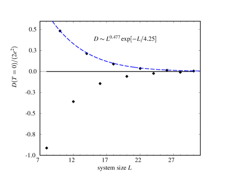
FIG. 1.: Scaling dependence of $D(T=0)$ at $U=4$ and half-filling.

Away from half-filling the Hubbard model describes an ideal metal, with a finite Drude weight at $L\rightarrow\infty$. We show the system size dependence at quarter filling in fig. 2. We find that the L-dependence is very similar to the half-filled case, shifted by $D(L=\infty)$. Even though eq. (19) was only derived for the half-filled case, it fits the approach to $D(L=\infty)$ very well, albeit with a different exponent for $L$ and a very large value of $\zeta$, as shown in the inset of fig. 2.

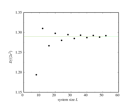
FIG. 2.: The Drude weight at $U\!=\!4$ and quarter filling $\nu\!=\!\frac{1}{2}$ scales towards a finite value $D(L\!=\!\infty)/$$(2e^{2})=1.29$. The inset shows the scaling dependence $(D(L=\infty)-D(L))/(2e^{2})$ $=L^{-1.12(1)}\exp[-L\cdot 0.04(1)]$ on a logarithmic scale (at $L\mbox{ mod }4=0$).

We determined the complete filling dependence of the Drude weight by solving the Bethe ansatz equations numerically for system sizes up to $L=80$, and extrapolating to infinite system size using eq. (19). The results are shown in fig. 3. As expected, the Drude weight vanishes for $\nu=0$ (no electrons) and $\nu=1$ ($L$ electrons). For small system sizes up to $L=12$ the filling dependence has already been reported by Fye et al. using Lanczos techniques [11]. Solving the Bethe ansatz equations enables us to access much larger systems (up to $L=80$) and thus to obtain a better extrapolation to the thermodynamic limit. The Drude weight for fixed system size $L=100$ has also been obtained by Römer and Punnoose [13], and our results agree.

FIG. 3.: The filling dependence of $D$ at $U=4$ and $T=0$, extrapolated to infinite system size.

B Partial Drude weight at finite temperature

We now turn to finite temperatures and half-filling. Whereas ground state properties depending only on the energy can be calculated easily using the Bethe ansatz equation eq. (12), dynamical properties are much harder to determine via the usual Bethe ansatz. One recent method by Klümper et al.  reduces the problem to finding the solution of two coupled nonlinear integral equations [23]. Here we will be content with a much simpler procedure to calculate the spin triplet contribution to the finite temperature Drude weight at half-filling. We neglect excitations across the charge gap. As we will see, this approximation is valid for small values of $LT/U$, i.e. for low temperatures and not too large systems.

Low energy excitations are described by variations of the quantum numbers around the ground state configuration. We choose $N\mbox{ mod }4=2$ whence the ground state is a singlet[10]. As excitations around this state we consider spin triplet states, with $M=N/2-1$, that is, we consider the $S=1$ and $S_{z}=-1$ excitations. To include singlet excitations one has to refer to the general Bethe ansatz equations introduced by Takahashi [24], with a phase included as in ref. [14]. The generalized equations describing all four branches of singlet and triplet excitations (the afore mentioned ones and the $S=1$ and $S_{z}=0$ excitations) are given in [25].
Due to the charge gap at half-filling, there are no low lying charge exitations. The charge quantum numbers $I_{n}$ therefore remain unchanged from the ground state. For the spin quantum numbers we get from eq. (15) with $M=N/2-$1 that

$$|J_{j}|\leq\frac{N}{4}\,,$$ (20)

and the $J_{j}$ are now half-integer. Thus there are $N/2+1$ possible values for the $M=N/2-1$ spin quantum numbers. All possibilities to distribute the $J_{j}$’s according to eq. (20) that differ from the ground state constellation describe excited states. These are the lowest possible excitations. In addition, there is a singlet excitation, degenerate in energy with the three triplet excitations[22]. This singlet excitation also contains two holes in the spin quantum numbers compared with the ground state constellation. It is described by complex quantum numbers. Due to the degeneracy, its contribution just multiplies the partition function by a constant factor.

The quantity $D^{triplet}(\beta,L)$ calculated via eq. (18) using only the triplet spin excitations is of course only part of the Drude weight, but as we will see it should be a good approximation for small temperatures and small system sizes.

For the temperature and system size dependence of $D^{triplet}(\beta,L)$ (at $L\mbox{ mod }4=2$) we find again a relation similar to the $T=0$ result of Stafford and Millis [10], eq. (19):

$$\frac{D^{triplet}(\beta,L)}{2e^{2}}\,=\,a(\beta)\,L^{b}\,\exp[-c\cdot L],$$ (21)

where only $a(\beta)$ is a function of the temperature. The results for $D^{triplet}$ are shown in fig. 4, and the fitted parameters $a$ and $c$ in table I.

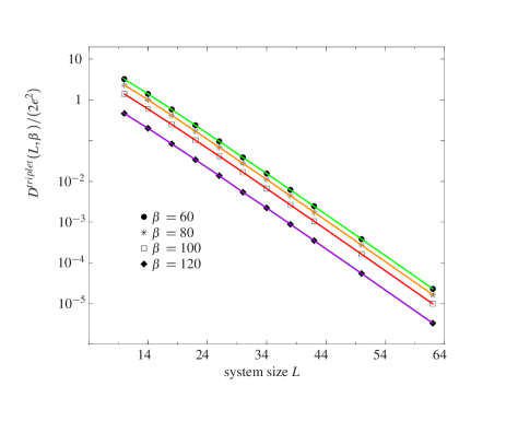
FIG. 4.: Scaling behavior of $D^{triplet}(T)$ as a function of $L$ for finite temperatures and $U=4$, $\nu=1$.

Inverse Temperature	$a$	$c$
$\beta=60$	$16.65\pm 0.16$	$0.2400\pm 0.0003\;$
$\beta=80$	$11.90\pm 0.11$	$0.2400\pm 0.0003\;$
$\beta=100$	$7.140\pm 0.068$	$0.2400\pm 0.0003\;$
$\beta=120$	$2.379\pm 0.023$	$0.2400\pm 0.0003\;$

TABLE I.: Parameters $a$ and $c$ obtained by fitting the curves in fig. 4 to eq. (21).

We conclude that in the thermodynamic limit, $L\rightarrow\infty$, triplet excitations do not contribute to the Drude weight. This also remains true for higher spin excitations [26].

For the $\beta$-range studied, the exponent $b=0.336\pm 0.005$ and the length scale $c^{-1}=4.17\pm 0.01$ are independent of temperature. They differ somewhat in value from the $T=0$ result for the complete Drude weight $D(T=0)$ (see eq. (19) and fig. 1). The amplitude $a(\beta)$ of $D^{triplet}$ is precisely linear in $\beta$ for the $\beta$-range studied.

$$a(\beta)=(30.911\pm 0.007)-(0.23771\pm 0.00009\,)\cdot\beta.$$ (22)

This is surprising, since it resembles the high temperature behavior generally expected of the complete Drude weight [1].

We found that the interaction dependence of $D^{triplet}$ for a given temperature and system size can be approximated by

$$D^{triplet}(U)\,\sim\,U^{-d}\cdot\exp[-f\cdot U],$$ (23)

where the parameters $d$ and $f$ depend on system size.

Recently we received a paper by Fujimoto et al.[15] with exact expressions for the Drude weight at finite temperature in the limit $L\rightarrow\infty$, based on the Bethe ansatz. The Drude weight is finite at finite temperature, in agreement with our results. The authors compute explicitely the leading contributions to D($L=\infty$,T) at small temperatures, which at half filling are, as expected, proportional to  $\exp[-\Delta_{MH}\beta]$, where $\Delta_{MH}$ is the Mott-Hubbard gap.

Since the quantity $D^{triplet}(\beta,L)$ vanishes exponentially as $L\rightarrow\infty$, the spin contributions to the Drude weight considered here should dominate over the charge excitations for mesoscopic systems with $\beta\gg 1$ (so that higher excitations are suppressed) and

$$cL\ll\beta U\,$$ (24)

i.e. for low temperatures $T$ and small values of $LT/U$.

V Finite Temperature: QMC results

In this section we present our results for the Drude weight at large finite temperature and compare them with the prediction for the temperature and system size dependence obtained in the previous section.

The simulations were carried out using the grand canonical Quantum Monte-Carlo method [27]. The calculation yields the current-current correlation function at discrete imaginary times $\tau_{i}$. Performing a fourier transformation results in the current-current correlation function at the bosonic Matsubara frequencies $i\omega_{n}$. The analytic continuation of this function onto real frequencies at zero momentum gives $\Lambda(0,\omega)$ of eq. (6). However, the analytic continuation is a numerically ill-conditioned problem, which we can avoid. As pointed out in section II, one can take the limit $\omega\rightarrow 0$ directly along the imaginary axis. We therefore calculate $D$ by fitting $\Lambda$ on the Matsubara frequencies. This is still an ill-conditioned problem when only information about a finite number of Matsubara frequencies is available. It is therefore important to use a fitting function with the proper analytical form.

From the analytic continuation of eq. (A4) it can be seen that $\Lambda(0,i\omega_{l})$ is a well-behaved function on the imaginary axis, namely a sum of Lorentz curves:

$$\Lambda(0,i\omega_{l})\,=\,\sum_{j}\,c_{j}\frac{\Delta_{j}}{\omega_{l}^{2}+\Delta_{j}^{2}}.$$ (25)

We approximate it by a finite series

$$\Lambda_{\rm{FIT}}(0,i\omega_{l})\,=\,\frac{a}{\omega_{l}^{2}\,+\,b^{2}}\,+\,\frac{c}{\omega_{l}^{2}\,+\,d^{2}}\,+\,\frac{e}{\omega_{l}^{2}\,+\,f^{2}},$$ (26)

and determine the constants $a,b,c,d,e,f$ by a $\chi^{2}$-fit. This ansatz fits the data very well. Fig. 5 shows an example of our fit. We find that the third term in eq. (26), $e/(\omega_{l}^{2}+f^{2})$, and often also the second term, do not contribute significantly, indicating that eq. (26) is a good approximation. However, it should be noted that the constants $a,c$ and $e$ are not identical to the differences of the energy eigenvalues of $H$ appearing in $\Lambda(0,i\omega_{l})$, since they result from a fit to a truncated series. We have verified that our procedure to calculate the Drude weight produces results compatible with those using the f-sum rule eq. (7), but with smaller errors.

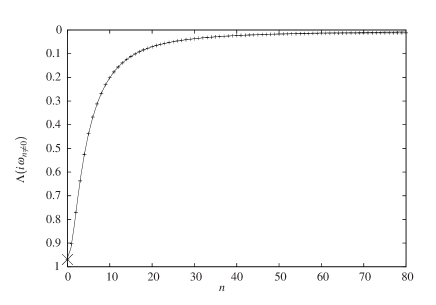
FIG. 5.: Fit of $\Lambda(0,i\omega_{n})$, at the nonzero Matsubara frequencies, for $L=32$, $U=4$, $\mu=2.2$ and $\beta=10$, plotted vs $n$. The cross marks the extrapolated value at $\omega=0$.

FIG. 6.: The Drude weight at $\beta=8$, $U=4$, $\nu=1$ is nonzero in the thermodynamic limit $L\rightarrow\infty$. The form of the interpolating function is motivated by the $T=0$ Bethe ansatz results.

We used this procedure to determine $D(T)$ from finite temperature Quantum Monte Carlo runs. We typically collected about $180000$ Monte Carlo sweeps for each data point, with a discrete time step of $\Delta\tau=1/32$ for $\beta=3$ and $\Delta\tau=1/10$ for $\beta=8$. We obtained the following results.

Fig. 6 shows the Drude weight for repulsive interaction $U=4$ and inverse temperature $\beta=8$. The system size dependence is compatible to that of $D^{triplet}(L)$, eq. (21), as expected for temperatures small compared to the charge gap.

$$D(L)/(\pi e^{2})\,=\,-A\cdot L^{-B}\exp[-C\cdot L]\,+\,d.$$ (27)

We determined the parameters by a $\chi^{2}$-fit. For the case shown in fig. 6 the result is $A=10.12\pm 1.14,\;B=0.75\pm 0.88,\;C=0.22\pm 0.09,$ and $d=0.020\pm 0.003$.

Thus, in the thermodynamic limit, we obtain a finite Drude weight $D(\beta=8,\nu=1,U=4)/(\pi e^{2})=0.02\pm 0.003$. The system size behavior of the full Drude weight $D(L,\beta=8)$ (eq. (27)) appears to be similar to that of the partial Drude weight $D^{triplet}(L,\beta)$ obtained by Bethe ansatz in eq. (21), within the large error of $B$, even though $D(L,\beta=8$) contains charge exitations, as well as higher spin and charge-spin-excitations.

Towards higher temperatures, the Drude weight increases rapidly. Results at $\beta=3$ are shown in fig. 7. The approach to the asymptotic value is very fast now, and there is no longer a clear exponential behavior.

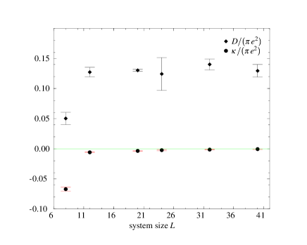
FIG. 7.: At large temperature ($\beta=3,U=4,\nu=1$) the Drude weight is large and converges rapidly with system size. The Meissner fraction $\kappa$ (see section VI) converges to zero quickly.

We checked that for lattice sizes $L=4n+2$ the finite value of the Drude weight remains the same within errors. One might be concerned that at temperature $\beta=3$ and lattice size $L=40$ the effects of the finite size gap could still be important. We therefore verified that at very high temperature ($\beta=0.5,L=20$) the Drude weight remains finite. In fact, its value increases further, to about $D/(\pi e^{2})=0.23(1)$. In fig. 8 our results for the Drude weight at various temperature in the half-filled case are shown.

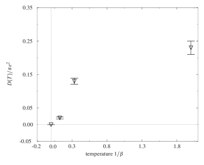
FIG. 8.: The Drude weight in the repulsive model ($U=4$,$\nu=1$) increases rapidly with temperature.

FIG. 9.: At quarter filling $\nu\approx 0.500$ ($\beta=3$, $U=4$) the Drude weight is finite. Small variations in filling of the grand canonical simulations may be responsible for the large deviation of the data at $L=28$.

Away from half-filling, the finite temperature Drude weight remains finite. Results at quarter filling are shown in fig. 9. The asymptotic value is already reached for very small system sizes. Note that away from half-filling, there was some fluctuation of the actual filling for different $L$ in the grand canonical QMC, which is not reflected in the error bars. This can cause the outlying point at $L=28$ in fig. 9.

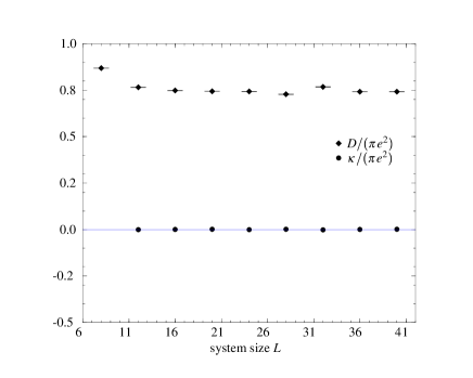
FIG. 10.: Attractive Hubbard model at high temperature: $\beta=3,~{}U=-4$, $\nu=1$. The Drude weight (upper points) quickly converges to a large finite value, whereas the Meissner fraction $\kappa$ vanishes (lower points; see section VI). For comparison: $\left\langle k_{x}\right\rangle\approx-0.890$, with little size dependence.

FIG. 11.: The Drude weight in the attractive model at lower temperature: $\beta=10,~{}U=-4,~{}\nu=1$ shows strong finite size dependence.

For the attractive Hubbard model at half-filling the situation is similar to the repulsive case. At low temperatures the system size dependence is slower, as shown in fig. 11, and the Drude weight has not yet reached its asymptotic value in our calculations. At high temperature, shown in fig. 10, the Drude weight converges quickly to a large value.

We see that in the half filled Hubbard model at finite temperature the Drude weight is non-zero in the thermodynamic limit $L\rightarrow\infty$, both for the repulsive and for the attractive case. Since half-filling is the insulating case of the Hubbard-model at zero temperature, this result is in disagreement with conjecture (2) (section III).

VI The Meissner Fraction

A property closely related to the Drude weight is the Meissner fraction $\kappa$ [28] defined as

$$\kappa\,\equiv\,\frac{\pi}{L}\frac{\partial^{2}F}{\partial\Phi^{2}}\Big{|}_{\Phi=0,\vec{q}\rightarrow 0},$$ (28)

where $F$ is the free energy. It reduces to Kohn’s Drude weight for $T=0$.

Evaluation of eq. (28) results in

$$\frac{\kappa}{\pi e^{2}}\,\,=\,-\,\left\langle k_{x}\right\rangle\,-\,\Lambda(\vec{q}\rightarrow 0,i\omega_{n}=0).$$ (29)

Note that $\Lambda(\vec{q}\rightarrow 0,i\omega_{n}=0)$ at the zeroeth Matsubara frequency, given in eq. (A5), is in general not equal to the analytically continued correlation function at $\omega\rightarrow 0$, eq. (A6), so that at finite temperature $\kappa$ differs from the Drude weight $D$ by the contributions from degenerate states

$$D(T)-\kappa=\lim_{\vec{q}\rightarrow 0}\frac{\beta}{L}\sum_{\stackrel{{\scriptstyle n,m}}{{E_{m}=E_{n}}}}P_{n}\left|\left\langle n\right|j^{p}(\vec{q})\left|m\right\rangle\right|^{2}.$$ (30)

In the thermodynamic limit $L\rightarrow\infty$ and in a transverse vector field, $\kappa$ measures the superfluid density [6, 16, 28]. In our one-dimensional case it will thus become zero. For a finite system, the Meissner fraction can be finite.

FIG. 12.: Meissner fraction in the repulsive model at low temperature: $\beta=8$ and $U=4,~{}\left\langle k_{x}\right\rangle\approx-0.955$, $\nu=1$. The two values at $L=10$ and $L=26$ differ in sign, since they belong to system sizes where $L=4\cdot n+2$.

FIG. 13.: Meissner fraction in the attractive model at low temperature, $\beta=10$, $U=-4,~{}\nu=1$: $\kappa\sim$ $\exp[-(0.1\pm 0.002)\cdot L]$. The kinetic energy is $~{}\left\langle k_{x}\right\rangle\approx-0.96$ for all system sizes.

We show results for the Meissner fraction on finite systems [16] in figures 7,10,12 and 13. For $L\rightarrow\infty$, $\kappa$ vanishes. We find a finite size behavior similar to that of the Drude weight. As for the Drude weight at $T=0$ (see fig. 1), $\kappa$ is positive when $L=4\,n+2$ and negative when $L=4\,n$. At high temperature $\beta=3$, $\kappa$ converges to zero very quickly both for the repulsive and for the attractive model (figures 7 and 10). At low temperature the approach to zero is exponential in system size, but much slower, as shown in figures 12 and 13. For very small systems, $\kappa$ is of similar magnitude as the Drude weight. Even though the difference $D-\kappa$, eq. (30), contains a factor of $\beta$, this difference turns out to be smaller at larger $\beta$ in the temperature range studied, both for small and for large systems, contrary to previous expectations [28].

VII Extended Hubbard model

In section V we showed that for the integrable Hubbard model eq. (3) the finite temperature Drude weight both at half-filling and away from it is nonzero even in the thermodynamic limit. This is in contrast to the $T=0$ case, where the Drude weight vanishes at half-filling due to the charge gap.

Let us now examine a nonintegrable case, provided by the extended Hubbard model with nearest neighbor interaction [19]

$$H_{e}\,=\,H_{H}\,+\,V\,\sum_{i}(n_{i\uparrow}+n_{i\downarrow})(n_{i+1\uparrow}+n_{i+1\downarrow}).$$ (31)

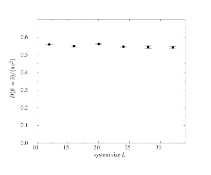
FIG. 14.: The Drude weight in the extended Hubbard model at at $U=4$, $V=1/2$, $\beta=3$ and $\nu=0.8978\pm 0.0002$ is nearly constant. The error bars do not take into account that the filling has some variation with $L$ in our grand canonical simulations.

We have measured the Drude weight and the Meissner fraction at finite temperature in this model. Results for a weak extended interaction of $V=1/2$ and away from half-filling are shown in fig. 14. The Meissner fraction drops to zero quickly, similar to the behavior in fig. 7. The Drude weight has a large value already at small system sizes. It shows a very slow falloff, consistent with $D\sim e^{-(0.00081\pm 0.00004)L}$. This falloff may entirely be caused by a very small systematic increase in the filling factor measured in the grand canonical simulations. If the exponential falloff is real, then the Drude weight would drop to small values only at extremely large system sizes, but would be zero in the thermodynamic limit, in agreement with the conjecture of Zotos et al.. However, from our data it appears more likely that the thermodynamic limit of $D$ is finite, which would be in disagreement with conjecture (3). This would imply that, even though the model is not integrable, there is an operator satisfying eq. (10) in the extended Hubbard model. A similar conclusion has been drawn for a related model recently [29].

We have also measured the Drude weight at $\beta=5,U=4$ and larger repulsion $V=1.6$, on a large system $L=60$. Both at quarter filling $\nu=0.5$ and at $\nu=0.633$ we find a finite value $D/(\pi e^{2})=0.21(2)$, even though the model is not integrable.

VIII Conclusions

We have presented results for the Drude weight $D(T)$, on mesoscopic systems and extrapolated to the thermodynamic limit, for zero and finite temperature in several versions of the 1D Hubbard model, including the dependence on system size, filling, and temperature.

At zero temperature we provided the full filling dependence of $D$, by solving the Bethe ansatz equations on large systems. For small finite temperatures we computed the dominant contribution to $D(T,L)$ on small systems from the Bethe ansatz. At larger finite temperature we used Quantum Monte Carlo. We showed that the Drude weight can be obtained by an extrapolation of the current-current correlation function purely in imaginary frequencies. We found a non-vanishing Drude weight at finite temperature for all cases considered, the repulsive Hubbard model both at and away from half-filling, the attractive model at half filling, and the extended Hubbard model away from half filling. The Drude weight quickly grows with temperature for the half filled Hubbard model.

Our results for the integrable half-filled Hubbard model do not confirm conjecture (2) (section III) on the connection between integrability and finite temperature Drude weight, and we find that conjecture (3) would disagree with the (likely) non-zero value of the Drude weight in the nonintegrable extended Hubbard-model.

A Spectral decomposition of the Drude weight

The Drude weight is given by

$$\frac{D(T)}{\pi e^{2}}\,=\,-\left\langle k_{x}\right\rangle\,-\,\mathop{\rm Re}\{\Lambda(0,\omega\rightarrow 0)\}$$ (A1)

at $\Phi=0$. Here $\left\langle k_{x}\right\rangle$ is the average kinetic energy per site and $\Lambda(\vec{q},\omega)$ is the current-current correlation function in frequency space [6]. It can be obtained from analytic continuation of

$$\Lambda(\vec{q},i\omega_{n})\,=\,\frac{1}{L}\int_{0}^{\beta}e^{i\omega_{n}\tau}\left\langle j^{p}(\vec{q},\tau)j^{p}(-\vec{q},0)\right\rangle\,d\tau$$ (A2)

where $\beta=1/T$, $i\omega_{n}=2\pi in/\beta$ are the Matsubara frequencies, $\vec{q}$ is the momentum of the applied external vector potential, and $e\,j^{p}(\vec{q})$ is the Fourier transform of the paramagnetic current density,

$$j^{p}(\vec{q})\,=\,i\,t\sum_{\begin{array}[]{l}{k=1,..,L}\\ {\sigma=\uparrow,\downarrow}\end{array}}\,e^{-i\vec{q}\vec{x}_{k}}\,(c^{\dagger}_{k+1,\sigma}c_{k,\sigma}\,-\,c^{\dagger}_{k,\sigma}c_{k+1,\sigma})\,.$$ (A3)

In an eigenbasis of the Hamiltonian eq. (3), the current-current correlation function at nonzero frequency is given by

$$\Lambda(\vec{q},i\omega_{l}\neq 0)=\,\hskip-8.61108pt\sum_{\begin{array}[]{c}{n,m}\\ {E_{n}\neq E_{m}}\end{array}}\hskip-8.61108pt\frac{P_{n}}{L}\frac{e^{(E_{n}-E_{m})\beta}-1}{i\omega_{l}+E_{n}-E_{m}}\left|\left\langle n\right|j^{p}(\vec{q})\left|m\right\rangle\right|^{2},$$ (A4)

and exactly at zero Matsubara frequency it is

$$\begin{array}[]{lllcl}\Lambda(\vec{q},i\omega_{l}\!=\!0)&=&\frac{2}{L}{\mbox{$\displaystyle\sum_{{\hskip-6.02777pt\begin{array}[]{c}{n,m}\\ {E_{n}\neq E_{m}}\end{array}\hskip-6.02777pt}}$}}&\frac{P_{n}}{E_{m}-E_{n}}&\left|\left\langle n\right|j^{p}(\vec{q})\left|m\right\rangle\right|^{2}\\[30.1388pt] &+&\frac{\beta}{L}{\mbox{$\displaystyle\sum_{{\hskip-6.02777pt\begin{array}[]{c}{n,m}\\ {E_{n}=E_{m}}\end{array}\hskip-6.02777pt}}$}}&P_{n}&\left|\left\langle n\right|j^{p}(\vec{q})\left|m\right\rangle\right|^{2}.\end{array}$$ (A5)

Here $\left\langle n|j^{p}|m\right\rangle$ are matrix elements of the current operator in the eigenbasis and $P_{n}=\exp(-\beta\,E_{n})$ denotes the Boltzman factor for the $n$th eigenvalue of the Hamiltonian.

The current-current correlation function is well defined [30] in the upper complex plane by specifying its values on an infinite set of finite Matsubara frequencies, eq. (A4). The analytic continuation can easily be performed by taking $i\omega_{l}\rightarrow\omega+i\delta$ in eq. (A4). Performing the zero frequency limit $\omega\rightarrow 0$ then yields

$$\mathop{\rm Re}\left(\Lambda(\vec{q},\omega\rightarrow 0)\right)\,=\,\frac{2}{L}\sum_{\stackrel{{\scriptstyle n,m}}{{E_{m}\neq E_{n}}}}\frac{P_{n}}{E_{m}-E_{n}}\,\left|\left\langle n\right|j^{p}(\vec{q})\left|m\right\rangle\right|^{2},$$ (A6)

which is identical to the first term in eq. (A5). Thus

$$\frac{D(T)}{\pi e^{2}}\,=\,-\left\langle k_{x}\right\rangle\,-\,\frac{2}{L}\sum_{\stackrel{{\scriptstyle n,m}}{{E_{m}\neq E_{n}}}}\frac{P_{n}}{E_{m}-E_{n}}\,\left|\left\langle n\right|j^{p}(0)\left|m\right\rangle\right|^{2}.$$ (A7)

Using second order perturbation theory and assuming that $\Phi$ removes all degeneracies, the expression takes the same form as eq. (9), so that then the two definitions eq. (2) and eq. (8) agree.
The second term in eq. (A5) is a nonanalytical part of the thermal Greens function [31], which does not contribute to the Drude weight, but instead to the Meissner fraction, discussed in section VI.

REFERENCES

- [1] H. Castella, X. Zotos, and P. Prelovšek, Phys. Rev. Lett. 74, 972 (1995).
- [2] X. Zotos and P. Prelovšek, Phys. Rev. B 53, 983 (1996).
- [3] X. Zotos, H. Castella, and P. Prelovšek, in Correlated Fermions and Transport in Mesoscopic Systems, proceedings of the XXXI Rencontres de Moriond Conference (1996).
- [4] X. Zotos, F. Naef, and P. Prelovšek, Phys. Rev. B 55, 11029 (1997).
- [5] W. Kohn, Phys. Rev. 133, A171 (1964).
- [6] D. J. Scalapino, S. R. White, and S. Zhang, Phys. Rev. B 47, 7995 (1993).
- [7] P. Kopietz, cond-mat/9709316.
- [8] G. Thomas, in High Temperature Superconductivity, ed. D. Tunstall and W. Barford (Adam Hilger, Bristol, 1991).
- [9] C. A. Stafford, A.J. Millis, and B. S. Shastry, Phys. Rev. B 43, 13660 (1990).
- [10] C. A. Stafford and A. J. Millis, Phys. Rev. B 48, 1409 (1993).
- [11] R. M. Fye, M. J. Martins, D. J. Scalapino, J. Wagner, and W. Hanke, Phys. Rev. B 44, 6909 (1991).
- [12] H.J. Schulz, Phys. Rev. Lett. 64, 2831 (1990).
- [13] R.A. Römer and A. Punnoose, Phys. Rev. B 52. 14809 (1995).
- [14] N.M.R. Peres, P.D. Sacramento, and J.M.P. Carmelo, cond-mat/9709144.
- [15] S. Fujimoto and N. Kawakami, J. Phys. A 31, 465 (1998).
- [16] The spatially constant on the ring employed here, as is customary, corresponds to a finite momentum for the electromagnetic vector potential in the three dimensional real space in which the ring is embedded. The momentum vanishes in the thermodynamic limit.
- [17] D. Poilblanc et al., Europhys. Lett. 22, 537 (1993).
- [18] M. V. Berry and M. Tabor, Prog. Roy. Soc. London A 356, 375 (1977).
- [19] G. Montambaux, D. Poilblanc, J. Bellissard, and C. Sire, Phys. Rev. Lett. 70, 497 (1993).
- [20] E. H. Lieb and F. Y. Wu, Phys. Rev. Lett. 20, 1445 (1968).
- [21] B. S. Shastry and B. Sutherland, Phys. Rev. Lett. 65, 243 (1990).
- [22] N. Andrei, ICTP Summer Course on Integrable Models in Condensed Matter Physics, in ”Low-dimensional Quantum Field Theories for Condensed Matter Physicists”, 1992; cond-mat/9408101.
- [23] G. Jüttner, A. Klümper, and J. Suzuki, cond-mat/9711310.
- [24] M. Takahashi, Prog. Theor. Phys. 47, 69 (1972).
- [25] J. M. P. Carmelo and N. M. R. Peres, Phys. Rev.B 56, 3717 (1997).
- [26] We thank the referee for pointing this out.
- [27] J. E. Hirsch, Phys. Rev. B 28, 4059 (1983).
- [28] T. Giamarchi and B. S. Shastry, Phys. Rev. B 51, 10915 (1995).
- [29] T. Prosen, cond-mat/9803358.
- [30] G. Baym and N.D. Mermin, J. Math. Phys. 2, 232 (1961).
- [31] P.C. Kwok and T.D. Schulz, J. Phys. C (Solid St. Phys.) Ser. 2, Vol. 2, 1196 (1969).