The McCoy-Wu Model in the Mean-field Approximation

Abstract

We consider a system with randomly layered ferromagnetic bonds (McCoy-Wu model) and study its critical properties in the frame of mean-field theory. In the low-temperature phase there is an average spontaneous magnetization in the system, which vanishes as a power law at the critical point with the critical exponents $\beta\approx 3.6$ and $\beta_{1}\approx 4.1$ in the bulk and at the surface of the system, respectively. The singularity of the specific heat is characterized by an exponent $\alpha\approx-3.1$. The samples reduced critical temperature $t_{c}=T_{c}^{av}-T_{c}$ has a power law distribution $P(t_{c})\sim t_{c}^{\omega}$ and we show that the difference between the values of the critical exponents in the pure and in the random system is just $\omega\approx 3.1$. Above the critical temperature the thermodynamic quantities behave analytically, thus the system does not exhibit Griffiths singularities.

1 Introduction

More than a quarter century ago McCoy and Wu [1] have introduced and partially solved a randomly layered Ising model on the square lattice. In the model, the nearest-neighbour vertical couplings $K$ are the same, whereas the horizontal couplings $J_{i}$ are identical within each column, but vary from column to column, such that they are taken independently from a distribution $\rho(J)\d{J}$. Recently, the solution of the McCoy-Wu (MW) model and the related random transverse-field Ising spin chain have been substantially extended by renormalization group [2] and numerical [3, 4, 5, 6] studies. Exact values for the average bulk $\beta$ and surface $\beta_{1}$ magnetization exponents and the $\nu$ correlation length exponent are given by:

$$\beta={3-\sqrt{5}\over 2},~{}~{}~{}\beta_{1}=1~{}~{}~{}{\rm and}~{}~{}~{}\nu=2\;,$$ (1)

which all differ from the corresponding values in the pure system. We note that several physical quantities of the MW model are not self-averaging at the critical point, consequently their typical and average values are different. Further curiosity of the MW model is the existence of Griffiths-McCoy singularities [7, 8] at both sides of the critical point, where the vertical spin-spin correlations decay as a power law with temperature-dependent decay exponents and, consequently, the susceptibility is divergent in a whole region.

The MW model, more precisely its quantum version, has been generalized for higher dimensions; namely quantum spin glasses in 2 and 3 space dimensions [9], the corresponding mean-field theory [10], diluted transverse Ising ferromagnets in higher dimensions [11] and random bond Ising ferromagnets in $d=2$ [12]. In all of these models, disorder is uncorrelated in the $d$ space dimensions and perfectly correlated in the additional imaginary time direction. Various analytical techniques, known from classical spin glasses [13], are at hand to treat the mean-field theory of other cases [10].

In this paper we consider a different type of generalization of the MW model to $d>2$ dimensions. In our approach the variation in the $J_{i}$ couplings remains one-dimensional and these couplings are identical in $(d-1)$-dimensional columns, while couplings in the other $(d-1)$-directions are the same, $K$. We study the problem within mean-field theory, therefore we call our system as Mean-Field McCoy-Wu (MFMW) model. We mention that inhomogeneous layered systems with quasi-periodic and smoothly varying interactions have been recently studied in the frame of mean-field theory by similar methods [14, 15].

The paper is organized as follows: In sec:sec2, we present the model and the numerical technique which is used to obtain the order parameter profile. The critical exponents are determined in sec:sec3, while in sec:sec4 an analysis of the critical temperature probability distribution is presented. Finally, in sec:sec5 we conclude with a relation between the values of the critical exponents in the pure and in the random systems.

2 Mean-Field McCoy-Wu model

As mentioned in the Introduction we consider a $d$-dimensional Ising model, which consists of $(d-1)$-dimensional layers, such that the Hamiltonian is given by:

$$H=-\sum_{i}\sum_{j}J_{i}\sigma_{i,j}\sigma_{i+1,j}-K\sum_{i}\sum_{<j,k>}\sigma_{i,j}\sigma_{i,k}\;.$$ (2)

Here $\sigma_{i,j}=\pm 1$ and $i=1,2,\dots,L$ characterises the position of the layers, whereas $j$ and $k$ give the position of the spin within a layer and $<j,k>$ are nearest neighbours. We treat the Hamiltonian in (2) in mean-field theory, then the local magnetization in the $i$-th layer, $m_{i}=<\sigma_{i,j}>$ (see fig1), is subject of variation, if the $J_{i}$ couplings are inhomogeneous. According to local mean-field theory the local magnetization satisfies the following set of self-consistency equations:

$$m_{i}={\rm tanh}\left[{J_{i-1}m_{i-1}+2(d-1)Km_{i}+J_{i}m_{i+1}\over T}\right]\;,$$ (3)

for $i=1,2,\dots,L$ and with $m_{0}=m_{L+1}=0$.

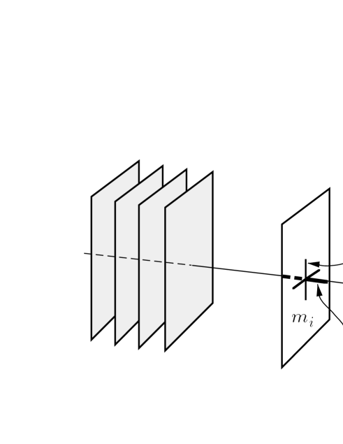
Figure 1: $d$-dimensional layered mean-field model

From here on we use units with $k_{B}=1$. The self-consistency equations in (3) have to be supplemented by boundary conditions (b.c.). Here we apply symmetry breaking b.c., such that the spins in one surface layer ($i=1$) are free, thus $J_{0}=0$, whereas in the other surface layer ($i=L$) they are fixed to the same state, thus $m_{L}=1$. The advantage of this type of b.c. is twofold:

i) one can study both the bulk and surface quantities at the same time, and

ii) one can investigate the profiles also at and above the critical temperature.

As we already mentioned the $J_{i}$ exchange couplings are quenched random variables. It is generally assumed that the average behaviour of the physical quantities does not depend on the details of the distribution of the couplings. In the following, we use the symmetric binary distribution:

$$\rho(J)={1\over 2}\delta(J-\lambda)+{1\over 2}\delta(J-\lambda^{-1})\;,$$ (4)

furthermore, to reduce the number of parameters we take $(d-1)K=\lambda$.

In this paper the MFMW model is studied numerically on finite slabs with relatively large width $(L\leq 1024)$, such that for a given random realization of the couplings the self-consistency equations in (3) are solved by the Newton-Raphson method. The resulting magnetization profile is then averaged over several $(\sim 10^{5})$ samples.

Figure 2: Averaged order-parameter profiles with free-fixed boundary conditions on a finite system of width $L=256$ at different temperatures below and around the critical temperature ($T_{c}^{av}=4.223$), for $\lambda=1.414$. The insert shows a specific disorder realization below $T_{c}^{av}$.

According to the numerical results, the MFMW model exhibits two phases which are separated by a critical point at $T_{c}^{av}$. Above the critical temperature, $T>T_{c}^{av}$, the average bulk magnetization is zero and the magnetization profile at $i=L$ drops to zero within the range of the surface correlation length $\xi_{\perp}\sim|T-T_{c}^{av}|^{-\nu}$, where $\nu$ denotes the corresponding critical exponent. Below the critical temperature, $T<T_{c}^{av}$, the average magnetization is finite at any site of the system. As seen in fig2 the average bulk magnetization $[m_{b}]_{av}$ corresponds to the value of $m$ in the plateau of the profile, which is different from the surface magnetization, and $[m_{b}]_{av}>[m_{1}]_{av}>0$. Again the width of the two surface regions, both at $i=1$ and $i=L$, are characterized by the corresponding correlation lengths.

3 Numerical determination of the critical exponents

The temperature dependence of the bulk and surface magnetization is shown in fig3. As seen in the figure both $[m_{b}]_{av}$ and $[m_{1}]_{av}$ vanish at the same temperature, thus we have the so-called ordinary surface transition [16]. The magnetizations close to the critical point are described by power laws in terms of the reduced temperature $t=T_{c}^{av}-T$ as $[m_{b}]_{av}(t)\sim t^{\beta}$ and $[m_{1}]_{av}(t)\sim t^{\beta_{1}}$, respectively. Indeed, as seen in the insert in fig3 the magnetizations versus reduced temperature in a log-log plot are asymptotically described by straight lines, the slope of those are given by the corresponding magnetization exponents.

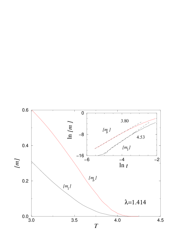
Figure 3: Temperature dependence of the average bulk and local surface magnetizations (disorder amplitude $\lambda=1.414$). The corresponding log-log plots are shown in the insert, where the dashed lines correspond to a linear fit leading to approximate values $\beta\approx 3.80$ and $\beta_{1}\approx 4.53$.

Having a closer look to fig3 one can notice that the magnetization close to the critical point exhibits log-periodic oscillations as a function of $t$ [17]. The origin of these oscillations is the existence of a finite energy scale in the binary distribution in binary, which is connected to the difference between the two possible values of the couplings $\lambda$ and $\lambda^{-1}$ [18]. We use these log-periodic oscillations to improve our estimates on the critical temperature and on the critical exponents, at the same time. The resulting reduced magnetization $[m_{b}]_{av}t^{-\beta}$ versus $t$ is presented in fig4 on a log-log plot, where we have taken optimized values for $\beta$ and $T_{c}^{av}$. In this figure we used the critical temperature to obtain perfect oscillations, whereas the correct value of the critical exponent $\beta$ is connected with a constant asymptotic limit of $[m_{b}]_{av}t^{-\beta}$ as $t\to 0$.

Figure 4: Rescaled average bulk magnetization at $\lambda=1.414$ with log-periodic oscillations, which are used to obtain refined estimates both on the critical temperature and on the critical exponent $\beta$.

The estimated critical temperatures, together with the bulk and surface magnetization exponents are given in Table 1 for different values of the parameter $\lambda$ of the binary distribution. As seen, the critical exponents do not depend on the strength of randomness and they agree, within the error of the estimates, with each other:

$$\beta=3.6(2)~{}~{},~{}~{}~{}\beta_{1}=4.2(2)\;.$$ (5)

We note that these exponents are unconventionally large, especially if we compare them with the similar ones of the pure model. A large $\beta$ exponent is connected with a fast variation of the magnetization around the critical point and the critical region in $t$, where the substantial variation of $[m]_{av}(t)$ takes place, is then very narrow. Therefore in a numerical calculation of the critical exponents one should approach closely the critical point, which in turn will lead to an increase of the error of the estimation. This fact explains the not very high accuracy of the numerical values in beta.

Table 1: Numerical values of the critical temperature and the magnetic exponents for the surface and bulk magnetizations.

$\lambda$	$T_{c}^{av}$	$\beta$	$\beta_{1}$
1.414	4.223	3.78	4.43
2.	4.969	3.60	4.33
3.162	6.908	3.51	4.26

The same fact, the relatively large values of the magnetization exponents, have made it very difficult to obtain a numerical estimate on the correlation length exponent $\nu$. In principle it can be determined from the decay of the magnetization profile at the critical point, which, according to the Fisher-de Gennes scaling theory [19] asymptotically behaves as:

$$[m(l)]_{av}\sim l^{-\beta/\nu}\;,$$ (6)

where $l=L-i$. For the MFMW model, however, due to the large value of $\beta$ the decay in decay is very fast and the profile will become smaller than the noise before its asymptotic regime is reached. Therefore we were not able to obtain a sensitive value for $\nu$.

Next we consider the specific heat of the system, the critical behaviour of which is deduced from the average internal energy:

$$[E]_{av}=-\sum_{i}\left[J_{i}m_{i-1}m_{i}+2(d-1)Km_{i}^{2}\right]_{av}\;,$$ (7)

as $C_{v}={1\over N}{\delta[E]_{av}\over\delta T}$. As seen in fig5 the specific heat at the critical point has a power law singularity and the corresponding critical exponent is obtained from the slope of the curve in a log-log scale as:

$$\alpha=-3.2(1)\;.$$ (8)

For the specific heat exponent, similarly to the magnetization exponents, we have made use of the log-periodic nature of the oscillations to increase the accuracy of the estimates. We note that the specific heat exponent in (8) is negative, thus it is decreased from its pure value $\alpha_{p}=0$ and consequently, due to randomness the specific heat has become less singular. The same observation was reported for a marginally aperiodic layered Ising model in mean-field theory [14].

Figure 5: Temperature dependence of the internal energy and corresponding log-log plot in insert. The different curves correspond to different chain sizes (from $L=32$ to 256) and the finite-size effects are quite small.

4 Probability distribution of the critical temperature

After having determined the average values of the physical quantities, which are accessible in a measurement, we are going to study their probability distributions. In this respect the distribution of the samples critical temperature $T_{c}$ is of primary importance. For a given random realization of the $J_{i}$ couplings, the critical temperature is obtained from selfeq in the limit $m_{i}\to 0$. Then one proceeds by replacing in the r.h.s. of (3) the ${\rm tanh}(x)$ by $x$ and solve the linear eigenvalue problem

$$\left(\matrix{a_{T}&J_{1}&0&&\dots&&0\cr J_{1}&a_{T}&J_{2}&&&&\cr 0&J_{2}&a_{T}&J_{3}&&&\cr&&J_{3}&a_{T}&\ddots&&\vdots\cr\vdots&&&\ddots&\ddots&J_{L-2}&0\cr&&&&J_{L-2}&a_{T}&J_{L-1}\cr 0&&&\dots&0&J_{L-1}&a_{T}\cr}\right)\left(\matrix{m_{1}\cr m_{2}\cr m_{3}\cr\vdots\cr m_{L-2}\cr m_{L-1}\cr m_{L}\cr}\right)=0\;,$$ (9)

for the critical temperature $T_{c}$, which is contained in the diagonal term, since $a_{T}=2(d-1)K-T_{c}$.

Figure 6: Probability distribution of the critical temperature and its behaviour: a) Distribution of the samples critical temperatures, b) Exponential fit of relative critical temperatures $t(i)=T_{c}^{max}-T_{c}(i)$, c) Exponential fit of the corresponding weigth $P(i)$.

The distribution of the samples critical temperature is shown in fig6a for the parameter $\lambda=2$ of the binary distribution binary, but similar type of behaviour is found for all other values of $\lambda$. As seen in fig6a the distribution consists of sharp peaks the widths of those is much smaller than the distance between them. We shall number the peaks by $i=0,1,\dots$ in descending order from the maximal one and denote by $T_{c}(i)$ the characteristic value of the critical temperature measured at the position of the tip of the peak. Thus we have $T_{c}(i=0)=T_{c}^{max}$ and $t(i)=T_{c}^{max}-T_{c}(i)$ measures the difference from the maximal critical temperature. First we note that, within the error of the calculation, the $T_{c}^{max}$ maximal critical temperature is equal to the average critical temperature

$$T_{c}^{max}=T_{c}^{av}\;,$$ (10)

which has been determined before from the behaviour of the average magnetization and the specific heat. We note that $T_{c}^{max}$ in (10) corresponds to the so called Griffiths temperature in random (Ising) spin systems, which is just the upper border of the Griffiths phase. In our system the observation in (10), i.e. $T_{c}^{max}$ and the Griffiths temperature coincides, means that there is no realization which exhibit finite bulk magnetization above the average critical temperature $T_{c}^{av}$. As a consequence the average quantities, such as the susceptibility, behave analytically above the critical temperature, thus there are no Griffiths singularities in the system. We note that similar observation is found in random systems with long range interactions, where mean-field theory is exact [10].

Figure 7: Power-law behaviour of the critical temperature distribution with respect to the difference from the maximal critical temperature, $t_{i}$, estimated at the successive peaks for different values of the disorder amplitude: $\lambda=1.414$ ($\times$), $\lambda=2.$ ($+$), and $\lambda=3.162$ ($\triangle$). The corresponding values of $\omega$ are given in the figure in the same order.

In the following we study the $t(i)=T_{c}^{max}-T_{c}(i)$ relative critical temperatures and the corresponding weigth $P(i)$ as a function of the index of the peak, $i$. As seen on fig6bc both quantities could be well fitted by exponential functions [20]:

$$t(i)\sim\exp(Ai)~{}~{},~{}~{}~{}P(i)\sim\exp(Bi)\;.$$ (11)

The $A$ and $B$ parameters in tP are found approximately independent of the form of the random distribution of the couplings and they ratio is given by:

$$\omega={B\over A}=3.1(1)\;.$$ (12)

Combining the two relations in tP we obtain a power law dependence of the $P(t_{i})=P(i)$ probability distribution:

$$P(t_{i})\sim t_{i}^{\omega}\;,$$ (13)

with $\omega$ given in omega. This relation is indeed well satisfied, as can be seen in fig7.

5 Relation between pure and random system critical exponents

In the following we use the form of the probability distribution in pt to relate the values of the critical exponents of the pure and the random systems. Generally we consider a physical quantity $Q(t)$, which behaves in the homogeneous system

$$Q(t)\sim t^{\epsilon_{p}}\;,$$ (14)

as a function of the reduced temperature $t=T_{c}-T$, for $|t|\ll 1$. (In mean-field theory for the bulk magnetization $\epsilon_{p}=\beta_{p}=1/2$, for the surface magnetization $\epsilon_{p}=\beta_{1_{p}}=1$ and for the specific heat $\epsilon_{p}=-\alpha_{p}=0$, etc.) We restrict ourselves to quantities with $\epsilon_{p}\geq 0$. To calculate the average behaviour of $Q(t)$ in the random system, we assume that in each random realization the temperature dependence $Q_{i}(t)$ is the same as in the pure system in (14) with the appropriate critical temperature $T_{c}(i)$ of the sample. This relation is then averaged over the samples:

$$[Q(t)]_{av}=\sum_{t_{i}>t}P(t_{i})Q_{i}(t)\sim\sum_{t_{i}>t}t_{i}^{\omega}(t_{i}-t)^{\epsilon_{p}}\sim t^{\omega+\epsilon_{p}}\;.$$ (15)

Thus the critical exponent in the random system, $\epsilon$, is related to its value in the homogeneous system as:

$$\epsilon=\epsilon_{p}+\omega\;.$$ (16)

This relation is indeed satisfied with all the considered physical quantities in eqs(5) and (8).

To summarize we have considered a generalized McCoy-Wu model and studied the critical properties in the mean-field approximation. We have determined different critical exponents and showed that they do not depend on the actual form of the coupling distributions. The values of the critical exponents in the pure and in the random systems are related and the only parameter which completely characterizes the random critical properties is the $\omega$ exponent of the probability distribution of the critical temperatures. We have seen in tcmax that the average critical temperature corresponds to the maximal critical temperature of the samples. Therefore above the $T_{c}^{av}$ critical temperature there are no samples with finite magnetization and hence there are no Griffiths singularities in the MFMW model.

The critical properties of the model are deeply connected to the probability distribution of the samples critical temperature in eqs (11) and (13). We consider it very probable that these expressions, which were observed numerically, can be obtained by analytical methods and perhaps also the $\omega$ exponent in (12) can be determined exactly.

This work has been supported by the French-Hungarian cooperation program ”Balaton” (Ministère des Affaires Etrangères-O.M.F.B.), by the Hungarian National Research Fund under grants No OTKA TO12830, OTKA TO23642 and OTKA TO25139 and by the Ministery of Education under grant No. FKFP 0765/1997. We thank the CIRIL in Nancy for computational facilities. We are indebted to H. Rieger and L. Turban for useful discussions.

References

References

- [1] B.M. McCoy and T.T. Wu, Phys. Rev. 176, 631 (1968); 188, 982(1969); B.M. McCoy, Phys. Rev. 188, 1014 (1969).
- [2] D.S. Fisher, Phys. Rev. Lett. 69, 534 (1992); Phys. Rev. B 51, 6411 (1995).
- [3] A. P. Young and H. Rieger, Phys. Rev. B 53, 8486 (1996).
- [4] F. Iglói and H. Rieger, Phys. Rev. Lett. 78, 2473 (1997).
- [5] A. P. Young, Phys. Rev. B 56, 11691 (1997).
- [6] F. Iglói and H. Rieger, Phys. Rev. B, in press (1998).
- [7] R.B. Griffiths, Phys. Rev. Lett. 23, 17 (1969).
- [8] B. McCoy, Phys. Rev. Lett. 23, 383 (1969)
- [9] H. Rieger and A.P. Young, Phys. Rev. Lett. 72, 4141 (1994); M. Guo, R.N. Bhatt and D.A. Huse, Phys. Rev. Lett. 72, 4137 (1994).
- [10] J. Miller and D.A. Huse, Phys. Rev. Lett. 70, 3147 (1993); N. Read, S. Sachdev and J. Ye, Phys. Rev. B52, 384 (1995).
- [11] T. Senthil and S. Sachdev, Phys. Rev. Lett. 77, 5292 (1996); T. Ikegami, S. Miyashita and H. Rieger, J. Phys. Soc. Jap. (in press).
- [12] H. Rieger and N. Kawashima, submitted to Phys. Rev. Lett.; C. Pich and A.P. Young, submitted to Phys. Rev. Lett.
- [13] K. Binder and A.P. Young, Rev. Mod. Phys. 58, 801 (1986).
- [14] P.E. Berche and B. Berche, \JPA 30, 1347 (1997).
- [15] F. Iglói and G. Palágyi, Physica A 240, 685 (1997).
- [16] K. Binder, in Phase Transitions and Critical Phenomena, vol 8; eds. C. Domb and J.L. Lebowitz, (London: Academic Press), p 1 (1983)
- [17] D. Karevski and L. Turban, \JPA 29, 3461 (1996).
- [18] Indeed there are no log-periodic oscillations, if the couplings follow uniform distribution, where no finite energy scale can be defined.
- [19] M.E. Fisher and P.-G. De Gennes, C.R. Acad. Sc. Paris B 287, 207 (1978).
- [20] Somewhat similar, exponential relation is present in the Sinai model (Ja. G. Sinai, Theor. Prob. Appl. 27, 247 (1982)), in a one-dimensional random walk in a random environment, where the time- and length-scales are related as . We can use analogous language for the MFMW model, if we notice that the eigenvalue matrix in \ereftc, which serves to determine the samples critical temperature, is equivalent to the transfer matrix of a one-dimensional directed walk, if a step of the walk on the -th site is weighted by a fugacity . The relevant time-scale of the problem is related to the gap at the top of the spectrum of the transfer matrix, which is connected to the relative critical temperature of the MFMW model as .