Polaron Problem by Diagrammatic Quantum Monte Carlo

Abstract

We present a precise solution of the polaron problem by a novel Monte Carlo method. Basing on conventional diagrammatic expansion for the Green function of the polaron, $G({\bf k},\tau)$, we construct a process of generating continuous random variables ${\bf k}$ and $\tau$, with the distribution function exactly coinciding with $G({\bf k},\tau)$. The polaron spectrum is extracted from the asymptotic behavior of the Green function. We compare our results for the polaron energy with the variational treatment of Feynman, and for the first time present precise dispersion curve which features an ending point at finite momentum.

PACS numbers: 71.38.+i, 02.70.Lq, 05.20.-y

The polaron problem has a very long history starting from the work by Landau [1]. In the most general form it is formulated as what happens to the particle when it is coupled to the environment, and what are the properties of the resulting object, called polaron, which consists of the bare particle dressed by environmental excitations. This problem arises over and over again not only because it is of fundamental importance both for the high-energy and for the condensed matter physics, but also because the notion of what we call “particles” becomes more diverse and new kinds of environments appear. In this paper we describe how the polaron problem can be solved numerically without systematic errrrs using diagrammatic Monte Carlo method, and present the solution of the notorious Fröhlich model (see, e.g., Refs. [2, 3]). First, we explain in detail how this model fits into the general Monte Carlo scheme [4, 5] dealing with distribution functions of continuous variables. We then describe the procedure of extracting the polaron spectrum, $E(k)$, from the asymptotic decay of the Green function. Although for small electron-phonon couplings the polaron energy, $E_{0}$, and the effective mass, $m_{*}$, i.e., the bottom of the polaron band, are rather well given by the perturbation theory, the perturbative approach fails to describe the spectrum near the threshold $E(k)-E_{0}\approx\omega_{p}$, where $\omega_{p}$ is the frequency of the optical phonon. In fact, the threshold features an ending point [6, 7]

$$E(k)=E_{0}+\omega_{p}-{(k-k_{c})^{2}\over 2m_{c}}~{}~{}~{}~{}~{}~{}~{}~{}(k<k_{c})\;,$$ (1)

analogous to the ending point of the excitation spectrum in ⁴He described by Pitaevskii [8]. Our numerical data unambiguously confirm this conclusion.

We start by considering the underlying mathematics. Suppose that for a certain random variable/set of variables, $y$, the distribution function ,$Q(y)$, is given in terms of a series of integrals with ever increasing number of integration variables:

$$Q(y)\,=\,\sum_{m=0}^{\infty}\sum_{\xi_{m}}\int dx_{1}\cdots dx_{m}\,F(\xi_{m},y,x_{1},\ldots,x_{m})\;.$$ (2)

Here $\xi_{m}$ indexes different terms of the same order $m$. The term $m=0$ is understood as a certain function of $y$. In Refs. [4, 5] it was shown how to arrange a Metropolis-type stochastic process simulating the distribution $Q(y)$ exactly. The process has very much in common with the Monte Carlo simulation of a distribution given by a multi-dimensional integral. Nevertheless, there is an essential difference associated with the fact that integration multiplicity in the expansion Eq. (2) is varying.

FIG. 1.: A typical diagram contributing to the polaron Green function.

Projection onto the polaron problem is as follows. Let us interpret the Matsubara (imaginary time) Green function of the polaron in the momentum-time representation, $G({\bf k},\tau)$, as the distribution function for the random variables ${\bf k}$ and $\tau$. We thus identify $G$ with $Q$, and $({\bf k},\tau)$ with $y$. Equation (2) is then identified with the diagrammatic expansion of $G({\bf k},\tau)$ in terms of free-electron and phonon propagators within the framework of conventional Matsubara technique at $T=0$. Then, the variables $x_{1},x_{2},\ldots,x_{m}$ are the internal times and independent momenta of the diagram $\xi_{m}$. A typical diagram is presented in Fig. 1. Solid lines denote the free-electron propagators, $G^{(0)}({\bf p},\tau_{2}-\tau_{1})=\exp[-(p^{2}/2-\mu)(\tau_{2}-\tau_{1})]$, where $\mu$ is the chemical potential. (Plank’s constant and electron mass are set equal to unity). Dashed lines and points stand for phonon propagators, $D({\bf q},\tau_{2}-\tau_{1})$, and vertexes of the electron-phonon coupling, $V({\bf q})$, respectively. Without loss of generality, one may fix the left end of the diagram at the origin of imaginary time, ascribing thus the time $\tau$ to the right end.

In this paper we confine ourselves to the Fröhlich model [2] where phonons are considered to be dispersionless, and the electron-phonon coupling has the form

$$H_{\mbox{e-ph}}\,=\,\sum_{{\bf k},{\bf q}}V({\bf q})\,\left(b^{{\dagger}}_{\bf q}-b_{-{\bf q}}\right)\,a^{{\dagger}}_{{\bf k}-{\bf q}}a_{\bf k}\;,$$ (3)

$$V({\bf q})\,=\,i\,\left(2\sqrt{2}\alpha\pi\right)^{1/2}\,\frac{1}{q}\;.$$ (4)

In Eq. (3) $a_{\bf k}$ and $b_{\bf q}$ are the annihilation operators for the electron with momentum $\bf k$ and for the phonon with momentum $\bf q$, respectively; $\alpha$ is a dimensionless coupling constant. In the Fröhlich model the phonon propagator is independent of momentum: $D({\bf q},\tau_{2}-\tau_{1})=\exp[-\omega_{p}(\tau_{2}-\tau_{1})]$. It is convenient, however, to attribute the vertex factors to the dashed lines, so that a dashed line with the momentum $\bf q$ contributes the factor $\tilde{D}({\bf q},\tau_{2}-\tau_{1})=\left|V({\bf q})\right|^{2}D(\tau_{2}-\tau_{1})$ to the diagram. The function $F$ is thus expressed as a product of $G^{(0)}$’s and $\tilde{D}$’s, in accordance with the standard diagrammatic rules.

Simulating the distribution $Q(y)$ is the process of sequential stochastic generation of diagrams, identical to functions $F$. (In our case these are the diagrams like that in Fig. 1, with certain fixed times and momenta.) The global process is constituted by a number of elementary sub-processes falling into two qualitatively different classes: (I) those which do not change the type of the diagram (change the values of variables of corresponding function $F$, but not the function itself), and (II) those which do change the structure of the diagram. The processes of the class I are rather straightforward, being identical to those of simulating continuous distribution corresponding to the given function $F$. In this paper we use only one process of this type, namely, shifting in time the right end of the diagram Fig. 1.

In the heart of the method are the sub-processes of type II. The generic rules for constructing them are as follows [5]. Suppose a certain sub-process $\cal A$ transforms a diagram $F(\xi_{m},y,x_{1},\ldots,x_{m})$ into $F(\xi_{m+n},y,x_{1},\ldots,x_{m},x_{m+1},\ldots,x_{m+n})$, and, correspondingly, its counterpart $\cal B$ performs the inverse transformation. For $n$ new variables we introduce vector notation: ${\vec{x}}=\{x_{m+1},x_{m+2},\ldots,x_{m+n}\}$. The process $\cal A$ involves two steps. First, it proposes a change, selecting a new type of diagram, $\xi_{m+n}$, and a particular value of $\vec{x}$. The vector $\vec{x}$ is selected with a certain distribution function $W(\vec{x})$. There are no requirements strictly fixing the form of $W(\vec{x})$, but to render the algorithm most efficient, it is desirable that $W(\vec{x})$ be chosen in accordance with some a priori knowledge of coarse-grained statistics of the vector $\vec{x}$. Upon proposing the modification, the process $\cal A$ either accepts it, with probability, $P_{\mbox{acc}}(\vec{x})$, or rejects. The process $\cal B$ either accepts a modification, removing variables $\vec{x}$ (with a certain probability $P_{\mbox{rem}}(\vec{x})$), or rejects this modification. For the pair of complimentary sup-processes to be balanced, the following Metropolis-like prescription should be fulfilled [5]:

$$P_{\mbox{acc}}(\vec{x})\>=\>\left\{\begin{array}[]{ll}R(\vec{x})/W(\vec{x}),\mbox{~{}~{}~{}~{}~{}~{}~{} if $R(\vec{x})<W(\vec{x})$}\;,\\ \;\;\;\;\;\;1\;,\mbox{~{}~{}~{}~{}~{}~{}~{}~{}~{}~{}~{}~{}~{}~{}~{}~{} otherwise}\;\;\;,\end{array}\right.$$ (5)

$$P_{\mbox{rem}}(\vec{x})\>=\>\left\{\begin{array}[]{ll}W(\vec{x})/R(\vec{x}),\mbox{~{}~{}~{}~{}~{}~{}~{} if $R(\vec{x})>W(\vec{x})$}\;,\\ \;\;\;\;\;\;1\;,\mbox{~{}~{}~{}~{}~{}~{}~{}~{}~{}~{}~{}~{}~{}~{}~{}~{} otherwise}\;\;\;,\end{array}\right.$$ (6)

where

$$R(\vec{x})\,=\,\frac{p_{\cal B}}{p_{\cal A}}\,\frac{F(\xi_{m+n},y,x_{1},\ldots,x_{m},{\vec{x}})}{F(\xi_{m},y,x_{1},\ldots,x_{m})}$$ (7)

and $p_{\cal A}$ and $p_{\cal B}$ are the probabilities of addressing to the sub-processes $\cal A$ and $\cal B$, which, in principle, may differ.

For solving the polaron problem it is sufficient to have only one pair of complementary processes of type II: the sub-process ${\cal A}$ adding a new phonon propagator to the diagram, and its counterpart ${\cal B}$ removing one phonon propagator from the diagram.

Consider the algorithm for the process ${\cal A}$. First we select the position $\tau_{1}$ for the left-hand end of the extra phonon propagator. This is done by choosing at random (with equal probabilities) one of the free-electron propagators, and by taking for $\tau_{1}$ any time (with equal probability density) within this propagator. Then we select the position $\tau_{2}$ for the right-hand end of the phonon propagator, in accordance with the distribution function $\propto\exp[-\omega_{p}(\tau_{2}-\tau_{1})]$. After that, we select the momentum for this propagator, using the distribution $\propto(1+q/q_{0})^{-2}$, where $q_{0}^{2}/2=\omega_{p}$. Now the proposing stage is completed, and we are ready to perform accept/reject step, following the above prescription, Eq. (5). The corresponding function $W({\vec{x}})$ (${\vec{x}}\equiv\{\tau_{1},\tau_{2},{\bf q}\}$) reads

$$W({\vec{x}})\,\propto\,\frac{1}{\tau_{0}}\,\frac{1}{(1+q/q_{0})^{2}}\,e^{-\omega_{p}(\tau_{2}-\tau_{1})}\;,$$ (8)

where $\tau_{0}$ is the length of the free-electron propagator, where the point $\tau_{1}$ is selected. As mentioned earlier, this form of $W$ is by no means the unique one. Apart from the factor $p_{\cal B}/p_{\cal A}$ which will be discussed later, the ratio (7) is now completely defined.

Consider now the algorithm for the process ${\cal B}$. We simply select at random (with equal probabilities) some phonon propagator and with the probabilities given in Eqs. (6), (8) remove it.

To complete the description of the sub-processes $\cal A$ and $\cal B$, we should define the ratio $p_{\cal B}/p_{\cal A}$. It is quite reasonable to address to the creation and annihilation procedures with equal probabilities. At the first glance it might seem that this immediately leads to $p_{\cal B}/p_{\cal A}=1$, but this is not true. The point is that when we select an electron propagator for placing the point $\tau_{1}$, we have $N_{e}$ equal chances, where $N_{e}$ is the number of free-electron propagators in the diagram being modified [denominator of Eq. (7) ], and when we select a phonon propagator for removing, we have $N_{ph}$ equal chances, where $N_{ph}$ is the number of phonon propagators in the diagram from which we try to remove the propagator [numerator of Eq. (7) ]. These $N_{e}$ and $N_{ph}$ are straightforwardly related to each other:

$$N_{ph}=(N_{e}+1)/2\;.$$ (9)

We thus get

$$\frac{p_{\cal B}}{p_{\cal A}}=\frac{N_{e}+1}{2N_{e}}=\frac{N_{ph}}{2N_{ph}-1}\;.$$ (10)

As for the processes of type I, these may include (i) selection of the time $\tau$ anywhere on the interval $(\tau_{2N_{ph}},\infty)$ according to the simple exponential distribution of $G^{(0)}({\bf k},\tau-\tau_{2N_{ph}})$ [obviously, the role of the chemical potential is to make this distribution normalizable, and the whole diagram not to diverge to $\tau\to\infty$; in fact, we use $\mu$ as a tuning parameter to probe different time-scales since the typical length of the diagram in time is controlled by the inverse of $E(k)-\mu$ ], and (ii) the change of the diagram momentum from ${\bf k}$ to ${\bf k+p}$ according to the distribution function $\exp[-(\bar{\bf k}+{\bf p})^{2}\tau/2m]$, where $\bar{\bf k}$ is the average electron momentum of the diagram, i.e., $\bar{\bf k}=\tau^{-1}\int_{0}^{\tau}d\tau^{\prime}\;{\bf k}(\tau^{\prime})$. We find it more convenient however, to select the incoming momentum at will and keep it fixed, since in this case we collect all the statistics to the value of $k$ we are interested in, instead of spreading it over the entire $k$-histogram.

FIG. 2.: Polaron Green function $G(k=0,\tau)$ for $\alpha=2$ and $\mu=-2.2$. Solid line is the exponential fit.

In Fig. 2 we show the typical data for the polaron Green function. Following Ref.[3], we use energy units such that $\omega_{p}=1$. After initial drop at short times we observe a pure exponential decay of $G({\bf k},\tau)$ at longer times (provided we are below the threshold of Cherenkov radiation, $E(k)-E_{0}<\omega_{p}$, so that the polaron state is stable). From the exponential asymptotic of the Green function we readily extract the polaron energy:

$$G(k,\tau\gg\omega_{p}^{-1})\,\to\,Z_{k}\exp[-(E(k)-\mu)\tau]\;.$$ (11)

By fine-tuning the chemical potential very close to $E(k)$ we may extend the time-scale for $G(k,\tau)$ which is given by $1/(E(k)-\mu)$. Typically, we had reliable statistics on the time-scale of order $100/\omega_{p}$, and were thus able to deduce the polaron energy to accuracy better than $0.01\omega_{p}$. Apart from the polaron energy, the asymptotic behavior of the Green function (11) gives us one more important physical characteristic of the polaron, the factor $Z_{k}$, which shows the fraction of the bare-electron state in the true eigenstate of the polaron:

$$Z_{k}\,=\,|\langle\mbox{free particle~{}}_{k}|\mbox{~{}polaron~{}}_{k}\rangle|^{2}\;.$$ (12)

FIG. 3.: Polaron energy $E_{0}$ as a function of coupling strength. Solid line is the Feynman’s variational result.

In Fig. 3 we present our results for the bottom of the band $E_{0}$ as a function of the coupling strength $\alpha$ in the most interesting intermediate region $0<\alpha\leq 6$. As expected, our precise data are below the solid line which gives the upper bound for $E_{0}$ (known to be the lowest ever obtained for this problem) as derived from the Feynman’s variational treatment [3]. We cannot but note the remarkable accuracy of the Feynman’s approach to the polaron energy.

However, the most interesting and instructive data are for the polaron spectrum at relatively large $k$. The perturbation theory result for the dispersion law, $E(k)\approx k^{2}/2-\alpha(\sqrt{2}/k)\sin^{-1}(k/\sqrt{2})$ (the solid line in Fig. 4), clearly demonstrates that the first-order correction is singular near the threshold of emitting the optical phonon and even develops an unphysical maximum (by assumption, the threshold point was defined as $E(k_{c})=E_{0}+\omega_{p}$; the maximum on the dispersion curve at $k<k_{c}$ is in contradiction with this assumption). One is bound to admit then that near the threshold the perturbation theory for the Fröhlich model fails at any $\alpha$ because of the singular phonon density of states, which is $\delta$-functional when one ignores the curvature of the phonon dispersion law $\omega_{p}(q)\approx\omega_{p}=const$ [6, 7] The formalism dealing with such cases was developed by Pitaevskii [8] for the ending point in ⁴He (a similar approach based on the Tamm-Dankoff approximation was suggested in Refs. [2, 9] and developed further in [6, 7]). By applying it to the Fröhlich model we arrive at the following equation for the dispersion law

$$\tilde{\omega}-a(k-k_{c})+b\tilde{\omega}\int{dx\over x^{2}-\tilde{\omega}}+R(k-k_{c},\tilde{\omega})\,=\,0\;,$$ (13)

where $\tilde{\omega}\equiv w-(E_{0}+\omega_{p})$, $R$ is a smooth function of $k-k_{c}$ and $\tilde{\omega}$, and $a$ and $b$ are some coefficients depending on $\alpha$ and $k_{c}$. This equation features an ending point at $k_{c}$, with the parabolic dependence Eq. (1) at $k<k_{c}$. The Monte Carlo data obtained for $\alpha=1$ are shown in Fig.4. We see how an almost perfect agreement with the perturbation theory for the band bottom transforms into non-perturbative behavior near $k_{c}$ predicted by Eq. (1).

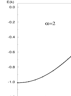
FIG. 4.: Polaron dispersion law for $\alpha=1$. Solid line is the first-order perturbation theory result.

Apparently, the ending-point is an artifact of the dispersionless phonon spectrum. With the non-zero curvature of $\omega_{p}(q)$ being taken into account, the ending point will transform into sharp crossover from zero to finite damping of the polaron state. We estimate the crossover region as $\Delta k/k_{c}\sim\sqrt{m/M}$ where $M$ is the mass of the host-lattice atoms.

In summary, we have presented the solution of the polaron problem by the diagrammatic quantum Monte Carlo method. The method directly simulates the polaron Green function (in the 4D momentum-time continuum), dealing with its conventional diagrammatic expansion. The polaron spectrum, extracted from the asymptotic behavior of the Green function, demonstrates essentially non-perturbative behavior at sufficiently large momenta.

It is worth noting that diagrammatic Monte Carlo approach applies to any model dealing with one/few degrees of freedom, either continuous or discrete, coupled to the thermal bath. Series of the form Eq. (2) naturally represent the partition function in the interaction picture [4, 5], and this approach was used recently to calculate the smearing of the Coulomb staircase in quantum dots at strong tunneling conductance [10]. More generally, diagrammatic Monte Carlo solves any problem which can be reduced to Eq. (2). The efficiency, however, severely depends on the sign problem, and the convergence becomes very poor if $F$-functions are not positive definite. It is thus of crucial importance to work in the representation in which the sign problem is absent.

We would like to thank N. Nagaosa, A. Furusaki, and Yu. Kagan for many fruitful discussions. We also would like to mention that the polaron problem was brought to our attention and suggested for solution by N. Nagaosa. We acknowledge the support from the Russian Foundation for Basic Research (Grant 98-02-16262).

REFERENCES

- [1] L.D. Landau, Sov. Phys., 3, 664 (1933).
- [2] H. Frhlich, H. Pelzer, and S. Zienau, Phil. Mag., 41, 221 (1950).
- [3] R.P. Feynman, Statistical Mechanics, Reading, Benjamin (1972); see also R.P. Feynman, Phys. Rev., 97, 660 (1955); T.D. Schultz, Phys. Rev., 116, 526 (1959).
- [4] N.V. Prokof’ev, B.V. Svistunov, and I.S. Tupitsyn, Pis’ma v Zh. Eksp. Teor. Fiz. 64, 853 [Sov. Phys. JETP Lett. 64, 911] (1996).
- [5] N.V. Prokof’ev, B.V. Svistunov, and I.S. Tupitsyn, to appear in Zh. Eksp. Teor. Fiz. (May 1998); cond-mat/9703200.
- [6] G.D. Whitfield and R. Puff, in Polarons and Exitons, eds. C.G. Kuper and G.D. Whitfield, Plenum Press, N.Y., 171 (1962); Phys. Rev., 139, A338 (1965).
- [7] D.M. Larsen, Phys. Rev., 144, 697 (1966).
- [8] L.P. Pitaevskii, Zh. Eksp. Teor. Fiz., 36, 1168 (1959).
- [9] D. Pines, in Polarons and Exitons, eds. C.G. Kuper and G.D. Whitfield, Plenum Press, N.Y., 155 (1962).
- [10] G. Göppert, H. Grabert, N. Prokof’ev, and B.V. Svistunov, submitted to Phys. Rev. Lett. (February 1998), cond-mat/9802248.