Phase Transitions in the Spin-Half $J_{1}$–$J_{2}$ Model

Abstract

The coupled cluster method (CCM) is a well-known method of quantum many-body theory, and in this article we present an application of the CCM to the spin-half $J_{1}$–$J_{2}$ quantum spin model with nearest- and next-nearest-neighbour interactions on the linear chain and the square lattice. We present new results for ground-state expectation values of such quantities as the energy and the sublattice magnetisation. The presence of critical points in the solution of the CCM equations, which are associated with phase transitions in the real system, is investigated. Completely distinct from the investigation of the critical points, we also make a link between the expansion coefficients of the ground-state wave function in terms of an Ising basis and the CCM ket-state correlation coefficients. We are thus able to present evidence of the breakdown, at a given value of $\frac{J_{2}}{J_{1}}$, of the Marshall-Peierls sign rule which is known to be satisfied at the pure Heisenberg point ($J_{2}=0$) on any bipartite lattice. For the square lattice, our best estimates of the points at which the sign rule breaks down and at which the phase transition from the antiferromagnetic phase to the frustrated phase occurs are, respectively, given by $\frac{J_{2}}{J_{1}}\approx 0.26$ and $\frac{J_{2}}{J_{1}}\approx 0.61$.

I Introduction

Antiferromagnetic materials have conveniently been modelled, since the early work of Heitler and London, as a lattice of magnetic atoms upon which the active electrons are localised. Furthermore, the exchange interactions between the electrons are conventionally described solely in terms of the spin degrees of freedom of the electrons. An archetypal model of this class remains the Heisenberg model in which only nearest-neighbour exchange interactions are included, and these are all taken to be equal. Although the Heisenberg model on the one-dimensional (1D) chain has been exactly solved many years ago by Bethe [1], it is still the case that relatively few other exact solutions have been found in the intervening 65 years or so to comparable models in higher dimensions or to models involving more complicated interactions, especially those containing an element of frustration.

On the other hand, various approximate numerical techniques have by now been applied to a large number of such magnetic lattice Hamiltonians. For example, many variational calculations have been undertaken, employing a wide variety of trial wave functions. Although these often give accurate upper bounds for the ground-state energy, for example, one often finds that the differences between the estimated energies for trial states of widely differing kinds are very small. Hence, predictions based on variational calculations for properties other than the energy, or to such questions as whether the exact ground state is ordered or disordered, are notoriously unreliable.

As a common alternative one may perform exact diagonalisations on small finite clusters of spins drawn from the infinite lattice under consideration. However, even with modern computers, one considers clusters of $N$ spins with $N\leq 36$. Extrapolation to the infinite lattice, $N\rightarrow\infty$, then needs to be performed. While exact results from finite-size scaling theory are often of great help in this regard, the extrapolation does need to be handled with great care. This is particularly true when using the results from finite clusters to make quantitative predictions for such quantities as the order parameter. Many wrong claims have been made in the past from an improper treatment of the very subtle phenomena which need to be taken into account in the extrapolations, as has been stressed and discussed with great care by Lhuillier and her co-workers [2]. Furthermore, one expects that such finite-cluster calculations will become less accurate the closer one approaches a quantum phase transition between states of different quantum order, marked by a critical value of some coupling parameter, at which a correlation length characterising the order typically diverges.

Results for much larger clusters are typically obtained by stochastic simulation of the many-body Schrödinger equation using various quantum Monte Carlo (QMC) algorithms. Where the basic spin-lattice Hamiltonian can be mapped onto an equivalent bosonic problem, as in the case of the Heisenberg model on a bipartite lattice, such QMC techniques can readily be applied to clusters containing several hundred or more spins, and very accurate results thereby obtained. In these cases, such as the Heisenberg model on the two-dimensional (2D) square lattice [3,4], the QMC results can usually be considered as “exact”, with the resulting errors arising only, or largely, from statistical errors which are open to systematic reduction within the limits of the available computing power.

What ultimately underpins these bosonic mappings, and what therefore makes such QMC simulations so readily attainable, is the knowledge that in some appropriate representation the multi-spin cluster coefficients describing the N-body wave function are all positive-definite. For example, in the case of the Heisenberg model on a bipartite lattice, this information is provided by the well-known Marshall-Peierls sign rule theorem [5].

Conversely, where such prior knowledge of the nodal structure of a many-body wave function is not exactly known, QMC calculations are beset by the notorious “minus-sign problem”, and are usually then much less reliable or much more difficult to implement with known algorithms. A typical way that such complications arise in spin-lattice problems is from the introduction of frustration. This can arise either from the geometry of the lattice under consideration or from the introduction into the Hamiltonian of competing exchange interactions. An example of the former is the basic Heisenberg model on a 2D triangular lattice; while an example of the latter arises from the introduction on a bipartite lattice of (antiferromagnetic) next-nearest-neighbour interactions in addition to the (antiferromagnetic) nearest-neighbour interactions of the pure Heisenberg model, resulting in the so-called $J_{1}$–$J_{2}$ model studied here.

Relatively few QMC calculations on such frustrated spin-lattice systems have been performed. As a starting point they typically require a good trial wave function, in terms of which the true wave function is well approximated, especially for its nodal surface structure. In such calculations there can still be a considerable systematic uncertainty, beyond the unavoidable statistical errors, which arises from whether the simulations have eliminated the bias inherent in the starting function. A typical recent calculation of this type was the fixed-node Green function Monte Carlo method [6] simulation of the spin-half 2D triangular-lattice Heisenberg antiferromagnet by Boninsegni [7].  While undoubtedly representing a very ambitious calculation of its kind, the resulting prediction for the sublattice magnetisation, which is the simplest measure of the antiferromagnetic Néel long-range order in this system, seems to be clearly too high by comparison with the results from the best of the alternative techniques, including exact diagonalisations of small clusters [2] and the coupled cluster method [8].  Furthermore, even the resulting QMC estimate for the ground-state energy of the triangular Heisenberg antiferromagnet gives an upper bound which is relatively easily bettered by the alternative techniques.

For such frustrated and similarly “difficult” systems, predictions based on even very large-scale QMC simulations share, at least to some extent, the uncertainties discussed above for variational calculations. In order to overcome these uncertainties, therefore, there is a real need to apply alternative semi-analytical approaches, especially those that have the demonstrated power to provide accurate predictions for the quantum order and for the positions and critical properties of any quantum phase transitions. One such method, namely the coupled cluster method (CCM) [9-19], stands to the fore in this respect. It has long been acknowledged as providing one of the most powerful, most widely applicable, and numerically most accurate at attainable levels of computational implementation, of all available ab initio formulations of microscopic quantum many-body theory. Furthermore, in recent years it has been widely applied to many spin-lattice Hamiltonians [8,20-33].  For example, very successful applications have by now been made to the solid phases of ${}^{3}He$ [20]; the isotropic Heisenberg and anisotropic $XXZ$ models in 1D and on the 2D square lattice, both for spin-half systems [20-28] and higher-spin systems [29]; and the spin-one Heisenberg-biquadratic model on the 1D chain [30]; as well as to such frustrated spin-half models as the $J_{1}$–$J_{2}$ model in 1D (and 2D) [31-33] and the 2D triangular-lattice anisotropic Heisenberg antiferromagnet [8,26,28].

In the present paper we apply the CCM specifically to investigate phase transitions in the spin-half $J_{1}$–$J_{2}$ model on (the 1D chain and, especially, on) the 2D square lattice. Our main aim is to use this model as an archetypal example for which no exact information is known for the nodal structure of the exact ground-state wave function, apart from the Marshall-Peierls sign-rule results in the pure Heisenberg limit. There is particular interest in studying whether the sign rule is preserved when weak next-nearest-neighbour exchange interactions are included and, if so, whether there is a critical coupling beyond which the sign rule breaks down. We believe that the CCM is an excellent prima facie candidate for such studies, since in virtually all previous applications to models for which the Marshall-Peierls sign rule holds, the theorem is exactly obeyed at virtually all levels of implementation in different CCM approximation schemes.

Finally, we are also interested in examining the phase transition points, as the strength of the next-nearest-neighbour interactions is varied, at which the Néel antiferromagnetic long-range order present in the 2D square-lattice case at the Heisenberg point vanishes; and in studying whether there is any relationship between the phase boundaries and the points at which the Marshall-Peierls sign rule breaks down. We note that any reliable information gained on the pattern of the signs of the multi-spin cluster coefficients in the decomposition of the ground-state wave function should be very useful for two distinct reasons, namely (i) for use in devising improved trial starting wave functions for future QMC calculations, and (ii) for spotting possible patterns for the signs of the cluster coefficients in different phases or different regimes of coupling constants. The latter could be used, inter alia, to suggest possible generalisations of the Marshall-Peierls sign rule, and thereby to motivate the search for the proofs of suitably generalised theorems. Any such generalisations would clearly have immediate impact for a next generation of QMC calculations.

The rest of this paper is organised as follows. In Sec. II we discuss the Marshall-Peierls sign rule and the CCM formalism. The sign rule is first outlined for the Heisenberg model on bipartite lattices, before we describe the $J_{1}$–$J_{2}$ model and previous results. The CCM formalism is then reviewed in very general terms before describing one means of applying it to the $J_{1}$–$J_{2}$ model. Results for the ground-state energy and staggered magnetisation are discussed in Sec. III, together with results on the breakdown of the Marshall-Peierls sign rule for the model. Finally, we present our conclusions in Sec. IV.

II The Marshall-Peierls Sign Rule and the CCM formalism

A The Sign Rule For The Spin-Half Heisenberg Antiferromagnet

In this section we consider the spin-half Heisenberg antiferromagnet (HAF) on a bipartite lattice, where the Hamiltonian is given by,

$$H=\sum_{\langle i,j\rangle}^{N}{\bf s}_{i}.{\bf s}_{j}~{},$$ (1)

and the index $i$ runs over all lattice points and $j$ runs over the nearest neighbours to $i$. The angular brackets indicate that we count each nearest-neighbour bond only once. We note that for a bipartite lattice we can divide the lattice into two sublattices such that if $i$ is on one particular sublattice then $j$ must be on the other and vice versa.

For the one-dimensional (1D) linear chain, there is an exact solution to this model via the Bethe Ansatz technique [1]. For the two-dimensional (2D) square-lattice HAF, there is no exact solution to this problem, though many approximate calculations, including those using various quantum Monte Carlo [3,4] (QMC) methods and exact series expansion [34] techniques, have been performed.

Although no exact solution is known for the 2D case stated here we note that there is an exact sign rule first derived by Marshall [5] (and which we shall refer to here as the Marshall-Peierls sign rule). The rule for the square lattice HAF is in fact an illustration of the more general Marshall-Peierls sign rule for the HAF on any bipartite lattice. This sign rule provides exact information regarding the signs of the expansion coefficients of the ground-state wave function in an Ising basis, which is denoted $\{|I\rangle\}$. The exact ground-state wave function for an $N$-body spin system may be written as,

$$|\Psi\rangle=\sum_{I}\Psi_{I}|I\rangle~{},$$ (2)

where $\{\Psi_{I}\}$ are the expansion coefficients. We now divide the bipartite lattice into its two sublattices, denoted $A$ and $B$, such that each nearest-neighbour site to an $A$ sublattice site is on the $B$ sublattice and vice versa. If the number of up spins on the $A$ sublattice is called $p_{I}$ then it is possible to show [5] that the coefficients $\{\Psi_{I}\}$ satisfy

$$\Psi_{I}=(-1)^{p_{I}}a_{I},$$ (3)

where the new coefficients $a_{I}$ are all positive. This exact information regarding the signs of the coefficients may be used to define the nodal surface of the wave function in this basis, and hence is of use in QMC calculations [3,4].

B The $J_{1}$–$J_{2}$ Model

We shall now discuss the spin-half $J_{1}$–$J_{2}$ model on the 1D linear chain and the 2D square lattice. The Hamiltonian is given by,

$$H=J_{1}\sum_{\langle i,j\rangle}^{N}{\bf s}_{i}.{\bf s}_{j}+J_{2}\sum_{\langle\langle i,k\rangle\rangle}^{N}{\bf s}_{i}.{\bf s}_{k}~{},$$ (4)

where the sum on $\langle i,j\rangle$ runs over all nearest-neighbour pairs of sites, counting each pair (or bond) once and once only; and the sum on $\langle\langle i,k\rangle\rangle$ similarly runs over all next-nearest-neighbour pairs of sites, again counting each pair (or bond) once and once only. We note that in order to consider a wide range of the coupling parameters $J_{1}$ and $J_{2}$, it is useful to introduce the variable $\omega$ such that $J_{1}\equiv{\rm cos}~{}\omega$ and $J_{2}\equiv{\rm sin}~{}\omega$.

In 1D, no exact solution has been found for general values of the coupling constants $J_{1}$ and $J_{2}$, though there are some exact solutions including the Heisenberg point ($J_{2}=0$) and a point at $J_{2}/J_{1}=0.5$ at which the ground-state is fully dimerised [35]. Previous coupled cluster method (CCM) [31-33] and density matrix renormalisation group (DMRG) [9] calculations have very successfully been carried out for this model. The phase diagram is complicated, with three distinct phases. These phases may be characterised for our purposes as ferromagnetic, antiferromagnetic, and frustrated. The ferromagnetic phase is a highly degenerate phase in which the ground-state energy is equal to that of the classical fully aligned state. There is a first-order phase transition at $J_{1}=0$ with negative $J_{2}$ to an antiferromagnetic phase. The antiferromagnetic phase classically has its energy minimised by the Néel state, and the quantum-mechanical phase transition point to the frustrated phase is at (or is very near to) $J_{2}/J_{1}=0.5$. The frustrated phase classically contains a spin ‘spiral’ state which has a periodicity which varies with the ratio of the coupling constants $J_{2}/J_{1}$. There is some evidence that this changing periodicity with $J_{2}/J_{1}$ might also be seen in the quantum-mechanical system [33,36].

For the square lattice there are no exact results, though approximate spin wave theory (SWT) [37] calculations, exact diagonalisations of finite-sized lattices [38], and CCM [31] calculations have been performed. The ferromagnetic to antiferromagnetic phase transition point is, as for the 1D case, at $J_{1}=0$ with negative $J_{2}$, and the antiferromagnetic to frustrated phase transition is believed to be near to $J_{2}/J_{1}=0.5$.

The Marshall-Peierls sign rule, as discussed in Sec. II.A, is true for the Heisenberg model on a bipartite lattice. It is simple to prove that it is also preserved for the $J_{1}$–$J_{2}$ model with negative $J_{2}$ and positive $J_{1}$. However, it is not in general true for positive $J_{2}$ and positive $J_{1}$. In fact, the results from 1D short-chain calculations [36] suggest that the breakdown occurs very near to the Heisenberg point, at $J_{2}/J_{1}=0.032\pm 0.003$. By contrast, finite-size lattice calculations [38] on the square lattice indicate that the sign rule at the Heisenberg point may well be preserved up to some critical value of $J_{2}/J_{1}$ in the $0.2\leq J_{2}/J_{1}\leq 0.3$.

C The CCM Formalism

In this article we wish to perform CCM calculations for the $J_{1}$–$J_{2}$ model in the antiferromagnetic regime. We now present a brief survey of the CCM formalism and note that a much fuller account of the formalism as applied to quantum spin-lattice problems has been given in Ref. [8]. A more extensive overview of the method and its applications has also been given in Ref. [17]. The starting point for any CCM calculation is the choice of a normalised model or reference state, denoted $|\Phi\rangle$. We define a complete set of mutually commuting, multi-spin creation operators $\{C_{I}^{+}\}$ with respect to $|\Phi\rangle$ such that any Ising state $|I\rangle$ may be obtained as

$$|I\rangle\equiv C_{I}^{+}|\Phi\rangle,$$ (5)

for an $N$-body spin system. The ground-state wave function has previously been written in Eq. (2) as a linear combination of the states $\{|I\rangle\}$, and we now introduce the usual CCM parametrisations of the ket and bra ground states which are given by,

$$|\Psi\rangle=e^{S}|\Phi\rangle S=\sum_{I\neq 0}{\cal S}_{I}C^{+}_{I}~{}~{};~{}~{}~{}~{}$$ ; (6)

$$\langle\tilde{\Psi}|=\langle\Phi|\tilde{S}e^{-S} ~{}~{};~{}~{}~{}~{} \tilde{S}=1+\sum_{I\neq 0}\tilde{\cal S}_{I}C^{-}_{I}~{}.$$ (7)

The ket-state correlation operator in Eq. (6) is, as we can see, formed from a linear combination of the creation operators $\{C_{I}^{+}\}$ multiplied with the relevant ket-state correlation coefficients $\{S_{I}\}$. The Hermitian adjoints of the multi-spin operators $\{C_{I}^{+}\}$ are the multi-spin destruction operators $\{C_{I}^{-}\}$, and the bra state in Eq. (7) is formed by the linear combination of these destruction operators multiplied with the corresponding bra-state correlation coefficients $\{\tilde{S}_{I}\}$. The bra and ket states, defined by Eqs. (6) and (7), are not manifestly Hermitian adjoints of each other and so the variational property of an upper bound on the ground-state energy is not preserved. However, we note that the Hellmann-Feynman theorem is preserved. We also note that since $\langle\Phi|C^{+}_{I}=0=C^{-}_{I}|\Phi\rangle$ by definition, we have the explicit normalisation relations, $\langle\Phi|\Psi\rangle=\langle\tilde{\Psi}|\Psi\rangle=\langle\Phi|\Phi\rangle=1$.

The ground-state expectation value of the energy may now simply be written using the Schrödinger equation, $H|\Psi\rangle=E_{g}|\Psi\rangle$, as,

$$E_{g}=\langle\Phi|e^{-S}He^{S}|\Phi\rangle~{}.$$ (8)

Equation (8) shows an example of the well-known similarity transform which plays a crucial role in the CCM formalism. We further note that the similarity transform of any quantum mechanical operator may be written in terms of a series of nested commutators, so that for the Hamiltonian $H$ we have

$$e^{-S}He^{S}=H+[H,S]+\frac{1}{2!}[[H,S],S]+\cdot\cdot\cdot~{}~{}~{}.$$ (9)

The infinite series of Eq. (9) terminates at finite order if the Hamiltonian $H$ contains sums of products of only finite numbers of single-body operators, as is almost always the case and is, indeed, true for the model considered here. We also note that each time we perform a commutation operation in Eq. (9) we produce a link or contraction, so that every single operator in each $S$ within the nested commutator expansion is directly linked to an operator in the original Hamiltonian. In this way the Goldstone linked cluster theorem is satisfied and the expectation value of the energy, as well as all other expectation values, are size-extensive (i.e., they are well defined in the asymptotic thermodynamic limit $N\rightarrow\infty$ at all levels of approximation for the operator $S$). Indeed, the CCM works from the outset in the thermodynamic limit.

We now wish to find values for the ket-state and bra-state correlation coefficients. We do this by defining the expectation value, $\bar{H}\equiv\langle\tilde{\Psi}|H|\Psi\rangle$, and by requiring that this quantity is a minimum with respect to the ket-state and bra-state correlation coefficients. Hence, we have,

$$\delta\bar{H}/\delta\tilde{{\cal S}}_{I}=0\Rightarrow\langle\Phi|C^{-}_{I}e^{-S}He^{S}|\Phi\rangle=0~{}~{} ~{}~{}~{}~{}\forall I\neq 0~{}~{};$$ , (10)

$$\delta\bar{H}/\delta{\cal S}_{I}=0\Rightarrow\langle\Phi|\tilde{S}e^{-S}[H,C^{+}_{I}]e^{S}|\Phi\rangle=0~{}~{} ~{}~{}~{}~{}\forall I\neq 0~{}~{}.$$ , (11)

This formalism is exact in the limit that we include all possible multi-spin cluster correlations within $S$ and $\tilde{S}$, though in any real application this is usually impossible. We therefore need to consider approximation schemes whereby the expansions of $S$ and $\tilde{S}$ in Eqs. (6) and (7) may be truncated to some finite or infinite subset of the full set of independent (fundamental) multi-spin configurations. The three most commonly employed schemes have been: (1) the SUB$n$ scheme, in which all correlations involving only $n$ or fewer spins are retained, but no further restriction is made concerning their spatial separation on the lattice; (2) the SUB$n$-$m$ sub-approximation, in which all SUB$n$ correlations spanning a range of no more than $m$ adjacent lattice sites are retained; and (3) the localised LSUB$m$ scheme, which retains all multi-spin correlations over distinct locales on the lattice defined by $m$ or fewer contiguous sites.

In the next subsection we consider the application of the CCM to the $J_{1}$–$J_{2}$ model in the antiferromagnetic regime.

D The CCM Applied to the $J_{1}$–$J_{2}$ Model

As stated in the previous section, the starting point for any CCM calculation is the choice of the model (or reference) state. Here, we choose the classical Néel state to be our model state, in accordance with previous CCM calculations [8,31], in order to study the antiferromagnetic regime of the $J_{1}$–$J_{2}$ model. We visualise the Néel state by again dividing the lattice into two sublattices, $A$ and $B$, on which each of the nearest-neighbours sites to a given sublattice site are on the other sublattice. We populate the $A$ sublattice with ‘up’ spins (i.e., eigenvectors of the $s^{z}$ operator with eigenvalue $+\frac{1}{2}$) and the $B$ sublattice with ‘down’ spins (i.e., eigenvectors of the $s^{z}$ operator with eigenvalue $-\frac{1}{2}$).

In order to perform a CCM calculation we would like to treat each site on an equal footing. We do this by performing a rotation [8,31,33] of the local axes of the spins on the $A$ sublattice (‘up’ spins) by $180^{\circ}$ about the $y$-axis such that all spins on each sublattice appear mathematically to point downwards (i.e., in these new local axes). Since this rotational transformation is a canonical one, it has no effect on the commutation relations. It does however have a number of consequences. Firstly, the Hamiltonian is re-written in the local coordinates as,

$$H = -J_{1}\sum_{\langle i,j\rangle}\biggl{[}s_{i}^{z}s_{j}^{z}+\frac{1}{2}s_{i}^{+}s_{j}^{+}+\frac{1}{2}s_{i}^{-}s_{j}^{-}\biggr{]}$$ (13)

$$+J_{2}\sum_{\langle\langle i,k\rangle\rangle}\biggl{[}s_{i}^{z}s_{k}^{z}+\frac{1}{2}s_{i}^{-}s_{k}^{+}+\frac{1}{2}s_{i}^{+}s_{k}^{-}\biggr{]}~{}.$$

We also note that the set of creation operators $\{C_{I}^{+}\}$ may now be formed purely from products of spin raising operators with respect to the rotated, ‘ferromagnetic’ model state. We write this expression for an $l$-spin cluster as $C_{I}^{+}\equiv s_{i_{1}}^{+}s_{i_{2}}^{+}...s_{i_{l}}^{+}$. Conversely, the destruction operators are now formed purely from the spin lowering operators in an analogous manner, where $C_{I}^{-}\equiv s_{i_{1}}^{-}s_{i_{2}}^{-}...s_{i_{l}}^{-}$.

The Marshall-Peierls sign rule for the Heisenberg model is also modified. We obtain a new and exact rule for the Hamiltonian of Eq. (13) in an expansion of the ground-state wave function in terms of an Ising basis, $\{|I\rangle\}$, in the local, rotated spin coordinates. The corresponding expansion coefficients, $\{\Psi_{I}\}$, must now be positive for all of the states labelled by $I$. (A proof of this statement is not given here, but it is made in exactly the same manner as that of Marshall [5].) The $\{\Psi_{I}\}$ coefficients are henceforth explicitly stated in relation to the Ising basis in the local, rotated spin coordinates.

We now wish to provide a link between the $\{\Psi_{I}\}$ coefficients, in terms of the local axes, and the CCM ground-state parametrisation of the ket state of Eq. (6). This is done by applying the destruction operator $C_{I}^{-}$, for a particular cluster defined by the index $I$, to the expressions for the ket-state wave function of Eqs. (2) and (6). Note we choose only one ordering out of the indices $\{i_{1},i_{2},...,i_{l}\}$ of the total of $N(l!)\nu$ possible equivalent orderings for $C_{I}^{-}$ on the lattice, where $\nu$ is a symmetry factor dependent on the lattice. We therefore write the $\{\Psi_{I}\}$ coefficients as,

$$\Psi_{I}=\langle\Phi|C_{I}^{-}e^{S}|\Phi\rangle~{}\equiv~{}\langle\Phi|s_{i_{1}}^{-}s_{i_{2}}^{-}...s_{i_{l}}^{-}~{}e^{S}|\Phi\rangle~{}.$$ (14)

Note that Eq. (14) contains the implicit assumption that the spin raising operators in $C_{I}^{+}$ of Eq. (5), which are used to define $|I\rangle$ with respect to $|\Phi\rangle$, have only one ordering with respect to permutations of the indices $\{i_{1},i_{2},...,i_{l}\}$.

Again, it should be noted that in practice one restricts the choice of the clusters contained within $S$ to some well-defined approximation scheme. To keep the calculations as self-consistent as possible, we restrict the choice of the $\{\Psi_{I}\}$ coefficients to be for only those Ising states defined in Eq. (5) which correspond to the clusters used in $S$.

In the next section we describe our results for the ground-state expectation values for high-order, approximate CCM calculations which are determined computationally [8]. We also detect critical points in the CCM equations which are taken to be signatures of phases transitions in the real system. Once the ket-state correlation coefficients are found it is then possible to obtain approximate results for the $\{\Psi_{I}\}$ coefficients, again via a computational approach, and we discuss CCM results concerning the breakdown of the Marshall-Peierls sign rule as a function of $J_{2}/J_{1}$.

III Results

A Ground-State Expectation Values

The ground-state energy of Eq. (8) is approximately obtained once the CCM equations are first derived and then solved for a particular approximation scheme and approximation level. Descriptions of the method are given in Refs. [31-33]. Details of how one may obtain a computational solution for high-order LSUB$m$ approximations is given in Ref. [8]. We simply quote the results here for this model using the Néel model state and the interested reader is referred to these articles.

The LSUB$m$ results for the ground-state energy of the 1D $J_{1}$–$J_{2}$ model converge very well over the range $-\pi/2\leq\omega\leq{\rm tan}^{-1}(0.5)$. We note that the LSUB10 results agree to within 1$\%$ of those obtained by extrapolating the results from exact diagonalisations for short chains [31] over this range, though we do not provide a plot of this here. In 2D, we see in Fig. 1 that our results are again extremely well converged over the range $-\pi/2\leq\omega\leq{\rm tan}^{-1}(0.5)$. In Table I results are given for the ground-state energy of the square lattice system as a function of $\frac{J_{2}}{J_{1}}\equiv{\rm tan}\omega$ for $-0.5\leq\frac{J_{2}}{J_{1}}\leq 0.5$ for the LSUB6 and LSUB8 levels of approximation.

We note that in 2D the CCM results for the ground-state energy display characteristic terminating points at certain critical values of $\omega$. At these points the second derivative of the ground-state energy with respect to $\omega$ may also be determined, and we note that at these critical values of $\omega$ this quantity diverges. This type of behaviour has been observed previously [8] and is associated with a phase transition in the real system. The critical value in 2D near to the ferromagnetic phase transition, denoted $\omega_{F}$, is given in Table II. We see that the LSUB$m$ results are clearly converging to the exact value of $\omega_{F}=-\pi/2$. It is known [31] that the SUB2 approximation predicts this point exactly in both 1D and 2D.

As is seen from the entries in Table II, the antiferromagnetic point, denoted $\omega_{A}$, is detected in 2D with the LSUB6, LSUB8, and SUB2 approximations. It is not observed within the LSUB4 approximation. We can see that the LSUB$m$ critical value of $\omega$ decreases with increasing truncation index $m$, and an simple extrapolation [8] in the limit $m\rightarrow\infty$ gives a value for the phase transition point of $\frac{J_{2}}{J_{1}}\approx 0.61$.

We now introduce the sublattice magnetisation, which characterises the degree of quantum order inherent in the CCM wave functions. By inserting the CCM parametrisations of Eqs. (6) and (7) we find,

$$M\equiv-\frac{2}{N}\sum^{N}_{k=1}\langle\tilde{\Psi}|s^{z}_{k}|\Psi\rangle=-\frac{2}{N}\sum^{N}_{k=1}\langle\Phi|\tilde{S}e^{-S}s^{z}_{k}e^{S}|\Phi\rangle~{}~{},$$ (15)

where $s^{z}_{k}$ is in the local coordinates of each sublattice. Evaluation of the sublattice magnetisation requires both the ket- and bra-state cluster correlation coefficients. The actual procedure to do this is straightforward, and is also described in more detail elsewhere [8].

The sublattice magnetisation in 1D is non-zero in the range $-\pi/2\leq\omega\leq{\rm tan}^{-1}(0.5)$, though we note (see [31]) that it is greater than zero but monotonically decreases with increasing LSUB$m$ approximation level for all $\omega$ in this range. The sublattice magnetisation is zero in the true solution of this model in 1D, and although the CCM LSUB$m$ (and SUB2 [31]) results are non-zero we expect that with increasing level of LSUB$m$ approximation this would be better reflected in the CCM solution.

Figure 2 illustrates that that the situation is much clearer in 2D. We can see that the sublattice magnetisation in Fig. 2 is converging to a non-zero value over essentially all of the range $-\pi/2\leq\omega\leq{\rm tan}^{-1}(0.5)$. We note that there are divergences in the sublattice magnetisation which are observed at precisely the same points as the critical points, $\omega_{F}$ and $\omega_{A}$, of the energy in 2D. This reinforces our conjecture that these critical points are reflections of phase transitions in the real system.

B The Breakdown of the Marshall-Peierls Sign Rule

We now consider the Marshall-Peierls sign rule for the spin-half $J_{1}$–$J_{2}$ model on the linear chain and the square lattice. We need to obtain the $\{\Psi_{I}\}$ coefficients, either analytically or computationally, in terms of the ket-state coefficients. We then solve the SUB2 or LSUB$m$ equations in order to obtain the ket-state correlation coefficients and hence to obtain approximate values for the $\{\Psi_{I}\}$ coefficients. Note that these calculations are approximate in the sense that we only retain certain correlations in $S$ with a well-defined approximation scheme, though we are already working in the infinite lattice or $N\rightarrow\infty$ limit.

We note that at each order of LSUB$m$ approximation it is possible to perform this process of matching the terms in $e^{S}$ in Eq. (14) to the configuration $C_{I}^{-}$ analytically. In Appendix A we present the exact form of the $\{\Psi_{I}\}$ coefficients in terms of the ket-state coefficients within the LSUB4 approximation scheme for the 1D linear chain. Furthermore, we see that each of the $\{\Psi_{I}\}$ coefficients corresponding to two-body correlations with respect to $|\Phi\rangle$ via Eq. (5), is exactly equal to the corresponding CCM two-body ket-state correlation operator $\{S_{I}\}$ for any approximation scheme used in $S$. This may be proven by noting that there are no one-body spin correlations allowed in $S$ (in order to preserve the conserved quantity $s_{T}^{z}=\sum_{i}^{N}s_{i}^{z}~{}$), and then by considering the series expansion of the exponential in Eq. (14).

To obtain higher-order $\{\Psi_{I}\}$ coefficients using Eq. (14) we may conveniently use a computational approach. This amounts to partitioning the configuration in $C_{I}^{-}\equiv s_{i_{1}}^{-}s_{i_{2}}^{-}...s_{i_{l}}^{-}$ into the multiples of $S$ in the series expansion of $e^{S}$ of Eq. (14). It is then possible to identify by simple computer algebra the configurations of the partitioned pieces (each referring to an $S$ in the series expansion of the exponential), and find a numerical value for the $\{\Psi_{I}\}$ coefficients once the CCM ket-state equations have been solved at specific values of $\omega$.

In both 1D and 2D, we find that (at all levels of approximation) the Marshall-Peierls sign rule is preserved for $\omega=-\pi/2|_{+}$ (i.e., in the antiferromagnetic regime). That is, all of the $\{\Psi_{I}\}$ coefficients are found to be positive. The sign is broken for $\omega=-\pi/2|_{-}$ (i.e., in the ferromagnetic regime) at which point at least one of the coefficients becomes negative. Note that the crossover occurs exactly at the phase boundary $\omega=-\pi/2$, and that this is one case where the breakdown of the Marshall-Peierls sign rule occurs at exactly the same place as the phase boundary. We note that there is a first-order phase transition at this point.

In 1D, we find that all the $\{\Psi_{I}\}$ coefficients are positive at the Heisenberg point for the SUB2 scheme and for LSUB$m$ schemes with $m\leq 8$. Above this LSUB$m$ level of approximation (i.e., for $m>8$) a few of the $\{\Psi_{I}\}$ coefficients (which are very small in magnitude) become negative. However, for example, at the LSUB12 level we find that these same coefficients, which are negative at the LSUB10 level, again become positive, though we find that other new coefficients (which are similarly small in magnitude) then become negative. These would in turn presumably become positive at a still higher level of approximation. Thus, the CCM is completely consistent with the sign rule for the Heisenberg model in 1D. This is encouraging as this model is quite challenging for the CCM with this model state, as our results for the sublattice magnetisation have shown. We may also compare the ratios of the magnitudes of the $\{\Psi_{I}\}$ coefficients to those obtained via short-chain calculations, as shown in Table III. (Note that we examine the ratios to eliminate short-chain normalisation factors.) We can see that the correspondence between CCM and short-chain calculations is good, though it appears that the CCM results are better converged at the LSUB10 and LSUB12 levels of approximation than those from the 12-spin and 16-spin chains. Short-chain calculations [36] indicate the breakdown of the Marshall-Peierls sign rule at $J_{2}/J_{1}=0.032\pm 0.003$, though our CCM results cannot give an accurate value for this breakdown point.

For the square lattice, the situation is found to be much clearer. The signs of the $\{\Psi_{I}\}$ coefficients are found to be positive at the Heisenberg point at all orders of LSUB$m$ approximation and also from the SUB2 approximation. A clear transition from all of the coefficients being positive to one of them becoming negative is seen, and we believe that this clearly indicates the onset of the breakdown of the Marshall-Peierls sign rule. The points at which the LSUB$m$ approximation predicts a breakdown, denoted $\omega_{M}$, are shown in Table II. We can see that a simple extrapolation of these points gives a value for the breakdown of the sign rule to be at $J_{2}/J_{1}\approx 0.26$ which is in good agreement with the SUB2 result of $J_{2}/J_{1}=0.2607$ and exact diagonalisations of finite-sized lattice calculations [38] which give a corresponding value of $J_{2}/J_{1}$ in the range of $0.2$–$0.3$. At SUB2 and LSUB4 levels of approximation it is the $\{\Psi_{I}$ } coefficients for the two-spin cluster with separation $\hat{x}+2\hat{y}$ that becomes negative first, where $\hat{x}$ and $\hat{y}$ are the unit vectors along the perpendicular axes of the square lattice. Higher-order CCM LSUB$m$ calculations predict, however, that the coefficients for other higher-order, highly-disconnected configurations first become negative at a slightly lower value of $\omega$ than the coefficient for this two-body configuration. This therefore indicates that higher-order multi-spin configurations might as be important as this two-body configuration in the breakdown of the sign rule for this model.

We note that the square-lattice results predict that the breakdown of the sign rule ($\omega_{M}$) occurs at a smaller value of $\omega$, at a particular approximation level, than the antiferromagnetic critical point ($\omega_{A}$) predicted by the CCM. In other words, the CCM results predict that there is a region of the antiferromagnetic regime in which the Marshall-Peierls sign rule is not being obeyed.

IV Conclusions

The CCM applied to the 1D spin-half $J_{1}$–$J_{2}$ model gives encouraging results for the ground-state energy, the critical points and the sublattice magnetisation. In this paper we have shown how the recent advances in the computational implementation of the method enable us to obtain useful results for the 2D model as well. We find that the 2D case is in many ways simpler than the 1D case, with more clearly defined critical points and a non-zero sublattice magnetisation.

We have also investigated the relation between the CCM and the Marshall-Peierls sign rule. In 1D we find the CCM results are consistent with the exact results in the region where these apply. In 2D we are able to obtain results which are better than the finite-size extrapolations and we can predict the point at which the sign rule fails. Our results indicate that this occurs at a different point than the phase transition from the simple antiferromagnet to the more complicated frustrated phase. We believe that the use of the exact Marshall-Peierls sign rules, extended by the CCM method into regions where it is not exact, can shed new light on the behaviour of this type of quantum spin system. Furthermore, it may provide information about the nodal surface that can be used for accurate QMC calculations in a much wider range of quantum spin systems than previously.

A Analytic Evaluation of the $\Psi_{I}$ Coefficients

We now present analytical expressions for the $\{\Psi_{I}\}$ coefficients in terms of the ket-state correlation coefficients in $S$ for the LSUB4 approximation in 1D. The ket-state correlation operator for the LSUB4 approximation in 1D is given by,

$$S=b_{1}\sum_{i}^{N}s_{i}^{+}s_{i+1}^{+}+b_{3}\sum_{i}^{N}s_{i}^{+}s_{i+3}^{+}+g_{4}\sum_{i}^{N}s_{i}^{+}s_{i+1}^{+}s_{i+2}^{+}s_{i+3}^{+}~{},$$ (A1)

where the index $i$ runs over all points on the linear chain. To obtain the $\{\Psi_{I}\}$ coefficients we now must choose the $C_{I}^{-}$ configurations in Eq. (14): for the nearest-neighbour, two-body coefficient, which we shall denote as $\Psi_{1}$, we use $C_{1}^{-}=s_{j}^{-}s_{j+1}^{-}$; for the third-nearest-neighbour, two-body coefficient, which we shall denote as $\Psi_{2}$, we use $C_{2}^{-}=s_{j}^{-}s_{j+3}^{-}$; and for the four-contiguous spin configuration coefficient, which we shall denote $\Psi_{3}$, we use $C_{3}^{-}=s_{j}^{-}s_{j+1}^{-}s_{j+2}^{-}s_{j+3}^{-}$. The result is therefore,

$$\Psi_{1} = b_{1}~{};$$ (A2)

$$\Psi_{2} = b_{3}~{};$$ (A3)

$$\Psi_{3} = b_{1}^{2}+b_{1}b_{3}+g_{4}~{}.$$ (A4)

The values of the $\Psi_{I}$ coefficients are independent of $j$, due to the translational symmetry of the lattice, and so the index $j$ is chosen arbitrarily from any of its $N$ possible values in order to obtain Eqs. (A2-A4). Higher-order LSUB$m$ approximations can be handled analogously by making use of computer-algebraic techniques.

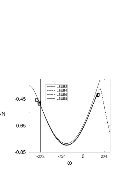
FIG. 1.: Results for the CCM ground-state energy of the spin-half $J_{1}$–$J_{2}$ model on the 2D square lattice, using the LSUB$m$ approximation based on the Néel model state, with $m=2,4,6,8$. LSUB$m$ critical points, $\omega_{F}$ and $\omega_{A}$, are indicated by the boxes. Note that $J_{1}\equiv{\rm cos}~{}\omega$ and $J_{2}\equiv{\rm sin}~{}\omega$.

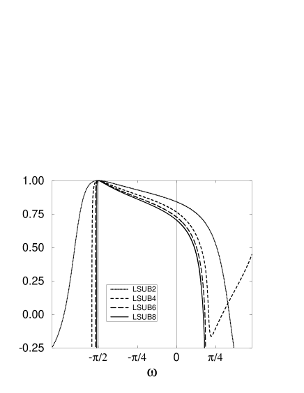
FIG. 2.: Results for the CCM sublattice magnetisation of the spin-half $J_{1}$–$J_{2}$ model on the 2D square lattice, using the LSUB$m$ approximation based on the Néel model state, with $m=2,4,6,8$. Note that $J_{1}\equiv{\rm cos}~{}\omega$ and $J_{2}\equiv{\rm sin}~{}\omega$.

TABLE I.: Results for the CCM ground-state energy of the spin-half $J_{1}$–$J_{2}$ model on the 2D square lattice as a function of $J_{2}/J_{1}={\rm tan}~{}\omega$, using the LSUB$m$ approximation based on the Néel model state, with $m=6,8$.

$J_{2}/J_{1}={\rm tan}(\omega)$	$E_{g}/N$  ($m$=6)	$E_{g}/N$  ($m$=8)
$-$0.50	$-$0.88237	$-$0.88353
$-$0.40	$-$0.83785	$-$0.83902
$-$0.30	$-$0.79393	$-$0.79510
$-$0.20	$-$0.75071	$-$0.75188
$-$0.10	$-$0.70833	$-$0.70951
0.00	$-$0.66700	$-$0.66817
0.10	$-$0.62699	$-$0.62816
0.20	$-$0.58868	$-$0.58988
0.30	$-$0.55271	$-$0.55397
0.40	$-$0.52012	$-$0.52164
0.50	$-$0.49311	$-$0.49551

TABLE II.: Results for the CCM critical points of the spin-half $J_{1}$–$J_{2}$ model on the 2D square lattice. The ferromagnetic and antiferromagnetic critical points are denoted $\omega_{F}$ and $\omega_{A}$ respectively. The point ($\omega>0$) at which the CCM predicts that the Marshall-Peierls sign rule breaks down for the square lattice is denoted $\omega_{M}$. Corresponding results for $(J_{2}/J_{1})|_{A}$ and $(J_{2}/J_{1})|_{M}$ are also shown, where $J_{2}/J_{1}={\rm tan}~{}\omega$.

	$\omega_{F}$	$\omega_{A}$	$(J_{2}/J_{1})|_{A}$	$\omega_{M}$	$(J_{2}/J_{1})|_{M}$
SUB2	$-\pi/2$	0.6416	0.7470	0.255	0.2607
LSUB4	$-$1.702	–	–	0.331	0.344
LSUB6	$-$1.628	0.583	0.660	0.290	0.298
LSUB8	$-$1.603	0.566	0.636	0.275	0.282
LSUB$\infty$	$-$1.572	0.544	0.605	0.255	0.261

TABLE III.: Results for the ratios of the magnitudes of the CCM LSUB$m$ $\Psi_{I}$ coefficients, for the spin-half, 1D Heisenberg model, compared to ratios of the magnitudes of the equivalent Ising expansion coefficients determined by finite-size, exact diagonalisations. The $\Psi_{1}$ coefficient is associated with the nearest-neighbour, two-body correlation with respect to the model state $|\Phi\rangle$; and $\Psi_{2}$, $\Psi_{3}$, and $\Psi_{4}$ are, respectively, the corresponding coefficients associated with the 3^rd-nearest-neighbour, two-body configuration, the four-contiguous-spin configuration, and the six-contiguous-spin configuration.

Ratio	12 Spins	16 Spins	LSUB10	LSUB12
$\frac{|\Psi_{3}|}{|\Psi_{1}|}$	0.7436	0.7163	0.6720	0.6758
$\frac{|\Psi_{2}|}{|\Psi_{1}|}$	0.1674	0.1552	0.1413	0.1381
$\frac{|\Psi_{4}|}{|\Psi_{1}|}$	0.4850	0.6155	0.5157	0.5248

REFERENCES

- [1] H. A. Bethe, Z. Phys. 71, 205 (1931); L. Hulthén, Ark. Mat. Astron. Fys. A 26, No. 11 (1938).
- [2] B. Bernu, C. Lhuillier, and L. Pierre, Phys. Rev. Lett. 69, 2590 (1992); B. Bernu, P. Lecheminant, C. Lhuillier, and L. Pierre, Phys. Rev. B 50, 10048 (1994); P. Lecheminant, B. Bernu, C. Lhuillier, and L. Pierre, Phys. Rev. B 52, 9162 (1995).
- [3] J. Carlson, Phys. Rev. B 40, 846 (1989); N. Trivedi and D.M. Ceperley, ibid. 41, 4552 (1990).
- [4] K.J. Runge, Phys. Rev. B 45, 12292 (1992); ibid. 45, 7229 (1992).
- [5] W. Marshall, Proc. R. Soc. London A 232, 48 (1955).
- [6] D.M. Ceperley and B.J. Alder, Phys. Rev. Lett. 45, 566 (1980); Science 231, 555 (1986); H.J.M. van Bemmel, D.F.B. ten Haaf, W. van Saarloos, J.M.J. van Leeuwen, and G. An, Phys. Rev. Lett. 72, 2442 (1995).
- [7] M. Boninsegni, Phys. Rev. B 52, 15304 (1995).
- [8] C. Zeng, D.J.J. Farnell, and R.F. Bishop, J. Stat. Phys., 90, 327 (1998).
- [9] F. Coester, Nucl. Phys. 7, 421 (1958); F. Coester and H. Kümmel, ibid. 17, 477 (1960).
- [10] J. Čižek, J. Chem. Phys. 45, 4256 (1966); Adv. Chem. Phys. 14, 35 (1969).
- [11] H. Kümmel, K.H. Lührmann, and J.G. Zabolitzky, Phys Rep. 36C, 1 (1978).
- [12] R.F. Bishop and K.H. Lührmann, Phys. Rev. B 17, 3757 (1978); ibid. 26, 5523 (1982).
- [13] J.S. Arponen, Ann. Phys. (N.Y.) 151, 311 (1983).
- [14] H.G. Kümmel, in Nucleon-Nucleon Interaction and Nuclear Many-body Problems, edited by S.S. Wu and T.T.S. Kuo (World Scientific, Singapore, 1984), p. 46.
- [15] R.F. Bishop and H. Kümmel, Phys. Today 40(3), 52 (1987).
- [16] J. Arponen, R.F. Bishop, and E. Pajanne, Phys. Rev. A 36, 2519 (1987); ibid. 36, 2539 (1987).
- [17] R.F. Bishop, Theor. Chim. Acta 80, 95 (1991).
- [18] R.F. Bishop, in Dirkfest ’92 – A Symposium in Honor of J. Dirk Walecka’s Sixtieth Birthday, edited by W.W. Buck, K.M. Maung, and B.D. Serot (World Scientific, Singapore, 1992), p. 21.
- [19] R.F. Bishop, in Many-Body Physics, edited by C. Fiolhais, M. Fiolhais, C. Sousa, and J.N. Urbano (World Scientific, Singapore, 1994), p. 3.
- [20] M. Roger and J.H. Hetherington, Phys. Rev. B 41, 200 (1990).
- [21] M. Roger and J.H. Hetherington, Europhys. Lett. 11, 255 (1990).
- [22] R.F. Bishop, J.B. Parkinson, and Y. Xian, (a) Phys. Rev. B 43, 13782 (1991); (b) Theor. Chim. Acta 80, 181 (1991); (c) Phys. Rev. B 44, 9425 (1991); (d) in Recent Progress in Many-Body Theories, edited by T.L. Ainsworth, C.E. Campbell, B.E. Clements, and E. Krotscheck (Plenum, New York, 1992), Vol. 3 p. 117; (e) J. Phys.: Condens. Matter 4, 5783 (1992).
- [23] F.E. Harris, Phys. Rev. B 47, 7903 (1993).
- [24] F. Cornu, Th. Jolicoeur, and J.C. Le Guillou, Phys. Rev. B 49, 9548 (1994).
- [25] R.F. Bishop, R.G. Hale, and Y. Xian, Phys. Rev. Lett. 73, 3157 (1994); Int. J. Quantum Chem. 57, 919 (1996).
- [26] C. Zeng, I. Staples, and R.F. Bishop, Phys. Rev. B 53, 9168 (1996).
- [27] R.F. Bishop, D.J.J. Farnell, and J.B. Parkinson, J. Phys.: Condens. Matter 8, 11153 (1996).
- [28] R.F. Bishop, Y. Xian, and C. Zeng, in Condensed Matter Theories, edited by E.V. Ludeña, P. Vashishta, and R.F. Bishop (Nova Science Publ., Commack, New York, 1996), Vol. 11 p. 91.
- [29] R.F. Bishop, J.B. Parkinson, and Y. Xian, Phys. Rev. B 46, 880 (1992).
- [30] R.F. Bishop, J.B. Parkinson, and Y. Xian, J. Phys.: Condens. Matter 5, 9169 (1993).
- [31] D.J.J. Farnell and J.B. Parkinson, J. Phys.: Condens. Matter 6, 5521 (1994).
- [32] Y. Xian, J. Phys.: Condens. Matter 6, 5965 (1994).
- [33] R. Bursill, G.A. Gehring, D.J.J. Farnell, J.B. Parkinson, T. Xiang, and C. Zeng, J. Phys.: Condens. Matter 7, 8605 (1995).
- [34] R.R.P. Singh, Phys. Rev. B 39, 9760 (1989); W. Zheng, J. Oitmaa, and C.J. Hamer, ibid. 44, 11869 (1991).
- [35] C.K. Majumdar and D.K. Ghosh, J. Math. Phys. 10, 1388 (1969); ibid. 10 1399 (1969).
- [36] Chen Zeng and J.B. Parkinson, Phys. Rev. B, 11609 (1995).
- [37] J. H. Xu and C. S. Ting, Phys. Rev. B 42, 6861 (1990); A. V. Chubukov and Th. Jolicoeur, ibid. 44, 12050 (1991).
- [38] J. Richter, N.B. Ivanov and K. Retzlaff, Europhysics Letters 25, 545 (1994); A. Voigt, J. Richter, N. B. Ivanov, Physica A 245, 269 (1997).