Driven Diffusive Systems:  An Introduction and Recent Developments

Abstract

Nonequilibrium steady states in driven diffusive systems exhibit many features which are surprising or counterintuitive, given our experience with equilibrium systems. We introduce the prototype model and review its unusual behavior in different temperature regimes, from both a simulational and analytic view point. We then present some recent work, focusing on the phase diagrams of driven bi-layer systems and two-species lattice gases. Several unresolved puzzles are posed.

1 Introduction

In nature, there are no true equilibrium phenomena, since all of these require infinite times and infinite thermal reservoirs or perfect insulations. Nevertheless, for a large class of systems, it is possible to set up conditions under which predictions from equilibrium statistical mechanics provide excellent approximations, as many of the inventions of the industrial revolution can attest to. By contrast, non-equilibrium phenomena are not only ubiquitous, but often elude the powers of the Boltzmann-Gibbs framework. Unfortunately, to date, the theoretical development of non-equilibrium statistical mechanics is at a stage comparable to that of its equilibrium counterpart in the days before Maxwell and Boltzmann. Using the intuition developed by studying equilibrium statistical mechanics, we are often “surprised” by the behavior displayed by systems far from equilibrium, even if they appear to be in time-independent states. For example, the well honed arguments, based on the competition between energy and entropy, frequently fail dramatically. In these lectures, we will present some explorations into the intriguing realm of non-equilibrium steady states, focusing only on a small class, namely, driven diffusive systems.

Motivated by both the theoretical interest in non-equilibrium steady states and the physics of fast ionic conductors [1], Katz, Lebowitz and Spohn [2] introduced a deceptively minor modification to a well-known system in equilibrium statistical mechanics: the Ising [3] model with nearest-neighbor interactions. In lattice gas language [4], the time evolution of this model can be specified by particles hopping to nearest vacant sites, with rates which simulate coupling to a thermal bath as well as an external field, such as gravity. If “brick wall” boundary conditions are imposed in the direction associated with gravity (particles reflected at the boundary, comparable to a floor or a ceiling), and if the rates obey detailed balance, then this system will eventually settle into an equilibrium state, similar to that of gas molecules in a typical room on earth. Although there is a local bias in the hopping rates (due to gravity), thermal equilibrium is established by an inhomogeneous particle density, at all $T<\infty$. However, if periodic boundary conditions are imposed, then translational invariance is completely restored so that, in the final steady state, the particle density is homogeneous, for all $T$ above some finite critical $T_{c}$, while a current will be present. Clearly, for gravity, such boundary conditions can be imposed only in art, as by M.C. Escher [5]. In physics, it is possible to establish such a situation with an electric field, e.g., by placing the $d=2$ lattice on the surface of a cylinder and applying a linearly increasing magnetic field down the cylinder xis. If the particles are charged, they will experience a local bias everywhere on the cylinder and a current will persist in the steady state. Echoing the physics of fast ionic conductors, we will therefore use the term “electric” field to describe the external drive and imagine our particles to be “charged”, in their response to this drive. This is the prototype of a “driven diffusive system.” Now, such a system constantly gains (loses) energy from (to) the external field (thermal bath), so that the time independent state is by no means an equilibrium state, à la Boltzmann-Gibbs. Instead, it is a non-equilibrium steady state, with an unknown distribution in general. As discovered in the last decade, modifying the Ising model to include a simple local bias leads to a large variety of far-from-simple behavior. The scope of these lectures necessarily limits us to only a bird’s eye view. Since a more extensive review has been published recently [6], we will restrict these notes to a brief “introduction” to this subject. Instead, we choose to include some developments since that review.

For completeness, we summarize, in Section II, the lattice model introduced by KLS and the Langevin equation believed to capture its essence in the long-time large-distance regime. The next section (III) is devoted to some of the surprising behavior displayed by this system, at temperatures far above, near, and well below $T_{c}$. A collection of recent developments is presented in Section IV. In the final section (V), we conclude with a brief summary.

2 The Microscopic Model and a Continuum Field Approach

On a square lattice, with $L_{x}\times L_{y}$ sites and toroidal boundary conditions, a particle or a hole may occupy each site. A configuration is specified by the occupation numbers $\{n_{i}\}$, where $i$ is a site label and $n$ is either 1 or 0. Occasionally, we also use spin language, defining $s\equiv 2n-1=\pm 1$. To access the critical point, half-filled lattices are generally used in Monte Carlo simulations: $\sum_{i}n_{i}=$ $L_{x}L_{y}/2$. The particles are endowed with nearest-neighbor attraction (ferromagnetic, in spin language), modeled in the usual way through the Hamiltonian: $H=-4J\sum_{<i,j>}n_{i}n_{j}$, with $J>0$. The external drive, with strength $E$ and pointing in the $-y$ direction, will bias in favor of particles hopping “downwards”. To simulate coupling to a thermal bath at temperature $T$, the Metropolis algorithm is typically used, i.e., the contents of a randomly chosen, nearest-neighbor, particle-hole pair are exchanged, with a probability $\min[1,e^{-(\Delta H-\epsilon E)/k_{B}T}]$. Here, $\Delta H$ is the change in $H$ after the exchange and $\epsilon=(-1,0,1)$, for a particle attempting to hop (against, orthogonal to, along) the drive. Note that these dynamic rules conserve particle number. For $E=0$, this system will eventually settle into an equilibrium state which is precisely the static Ising model [3, 4]. In the thermodynamic limit, it is known to undergo a second order phase transition at the Onsager critical temperature $T_{c}(0)=(2.2692..)J/k_{B}$. When driven ($E\neq 0$), this system displays the same qualitative properties, i.e., there is a disordered phase for large $T$, followed by a second order transition into a phase-segregated state for low $T$. However, with more scrutiny, this superficial similarity gives way to puzzling surprises. In particular, $T_{c}(E)$ appears to be monotonically increasing with $E$, saturating at about $1.41T_{c}(0)$ [7] for $E\gg J$. Why should $T_{c}(\infty)>T_{c}(0)$ be surprising? Consider the following “argument”. For very large $E$, hopping along $y$ becomes like a random walk, in that $\Delta H$ is irrelevant for the rates. Therefore, hops along $y$ might as well be coupled to a thermal bath at infinite $T$ (apart from the bias). Indeed, recall that our system gains energy from $E$ and loses it to the bath, so that any drive may be thought of as a coupling to a second reservoir with higher temperature. Then, it seems reasonable that $T$ must be lowered to achieve ordering, since this extra reservoir pumps in a higher level of noise, helping to disorder the system! To date, there is neither a convincing argument nor a computation which predicts the correct sign of $T_{c}(E)-T_{c}(0)$, let alone the magnitude. In the next Section, we will briefly review other puzzling discoveries, only a few of which are understood.

To understand collective behavior in the long-time and large-scale limit, we often rely on continuum descriptions, which are hopefully universal to some extent. Successful examples include hydrodynamics and Landau-Ginzburg theories. Certainly, the $\varphi^{4}$ theory, enhanced by renormalization group techniques, offers excellent predictions for both the statics and the dynamics near equilibrium of the Ising model. Following these lines, we formulate a continuum theory for the KLS model, in arbitrary dimension $d$. In principle, such a description can be obtained by coarse-graining the microscopic dynamics [8] but we will pursue a more phenomenological approach here. Seeking a theory in the long-time, large wavelength limit, we first identify the slow variables of the theory. These are typically

• ordering fields which experience critical slowing down near $T_{c}$, and

• any conserved densities.

The KLS model is particularly simple since it involves a single ordering field, namely the local “magnetization” or excess particle density, $\varphi({\bf x},t)$, which is also the only conserved quantity. Here, ${\bf x}$ stands for $(x_{1},x_{2},...,x_{d-1},x_{d}=y)$. The last entry denotes the one-dimensional “parallel” subspace selected by $E$. Thus, we begin with a continuity equation, $\partial_{t}\varphi+\nabla{\bf j}=0$, and postulate an appropriate form for the current ${\bf j}$. In the absence of $E$, it simply takes its Model B [9] form, ${\bf j}({\bf x},t)=-\lambda\nabla\frac{\delta{\cal H}}{\delta\varphi}+{\bf\eta(x},t)$, with the Landau-Ginzburg Hamiltonian ${\cal H=}\int\{\frac{1}{2}(\nabla\varphi)^{2}+\frac{\tau}{2}\varphi^{2}+\frac{u}{4!}\varphi^{4}\}$. As usual, $\tau\propto T-T_{c}$ and $u>0$. While the first contribution to ${\bf j}$ is a deterministic term, reflecting local chemical potential gradients, the second term, ${\bf\eta}$, models the thermal noise. The noise is Gaussian distributed, with zero mean and positive second moment proportional to the unit matrix, i.e., $<\eta_{i}\eta_{j}>=2\sigma\delta_{ij}\delta({\bf x}-{\bf x}^{\prime})\delta(t-t^{\prime})$, $i,j=1,...,d$. In the presence of $E$, we should expect at least two modifications to ${\bf j}$, namely first, an additional contribution ${\bf j}_{E}$ modeling the nonvanishing mass transport through the system and second, the generation of anisotropies, since $E$ singles out a specific direction. By virtue of the excluded volume constraint, the “Ohmic” current ${\bf j}_{E}$ vanishes at densities $1$ and $0$, corresponding to $\varphi=\pm 1$. Writing ${\cal E}$ for the coarse-grained counterpart of $E$, pointing along unit vector ${\bf\hat{y}}$, the simplest form is therefore ${\bf j}_{E}={\cal E}(1-\varphi^{2})[1+O(\varphi)]{\bf\hat{y}}$, where the $O(\varphi)$ corrections will turn out to be irrelevant for universal properties. Next, we consider possible anisotropies. Clearly, all $\nabla^{2}$ operators should be split into components parallel ($\partial^{2}$) and transverse ($\nabla_{\bot}^{2}$) to $E$, accompanied by different coefficients. For example, the anisotropic version of the Model B term $\tau\nabla^{2}\varphi$ will read $(\tau_{\|}\partial^{2}+$ $\tau_{\bot}\nabla_{\bot}^{2})\varphi$, with two different “diffusion” coefficients for the parallel and transverse subspaces. Should we expect both of these to vanish as $T$ approaches $T_{c}(E)$? Or just one of them - but which one? Recalling that the lowering of $\tau$, in the equilibrium system, is a consequence of the presence of interparticle interactions, we argue that $E$, stirring parallel jumps much more effectively than transverse ones, should counteract this effect in the parallel direction, having less of an impact in the transverse subspace. Thus, we anticipate that generically $\tau_{\|}>\tau_{\bot}$, so that criticality, in particular, is marked by $\tau_{\bot}$ vanishing at positive $\tau_{\|}$. This is borne out by the structure of typical ordered configurations, namely, single strips aligned with $E$, indicating that “antidiffusion”, i.e., $\tau_{\bot}<0$, dominates in the transverse directions below $T_{c}$. Finally, the drive also induces anisotropies in the noise terms so that the second moment of their distribution should be taken as $<\eta_{i}\eta_{j}>=2\sigma_{i}\delta_{ij}\delta(x-x^{\prime})\delta(t-t^{\prime})$. Since the transverse subspace is still fully isotropic, we define $\sigma_{1}=...=\sigma_{d-1}\equiv\sigma_{\|}$. Generically, however, we should expect $\sigma_{d}\equiv\sigma_{\bot}\neq$ $\sigma_{\|}$. Summarizing, we write down the full Langevin equation:

$$\partial_{t}\varphi({\bf x},t) = \lambda\{(\tau_{\bot}-\nabla_{\bot}^{2})\nabla_{\bot}^{2}\varphi+(\tau_{\|}-\partial^{2})\partial^{2}\varphi-2\alpha_{\times}\partial^{2}\nabla_{\bot}^{2}\varphi+$$ (1)

$$+\frac{u}{3!}(\nabla_{\bot}^{2}+\kappa\partial^{2})\varphi^{3}+{\cal E}\partial\varphi^{2}\}-\nabla{\bf\eta(x},t)\qquad,$$

with noise correlations

$$<\eta_{i}({\bf x},t)\eta_{j}({\bf x}^{\prime},t^{\prime})>=2\sigma_{i}\delta_{ij}\delta(x-x^{\prime})\delta(t-t^{\prime})\qquad.$$

This equation forms the basis for the analytic study of the KLS model. Fortunately, we need not be concerned about the detailed dependence of its coefficients on the microscopic $T$, $J$, and $E$. While they are in principle calculable within an explicit coarse-graining scheme, the properties that we already outlined above suffice for our purposes. Moreover, it turns out that we can simplify the most general form, (1), depending on the temperature regime considered. We will return to this discussion in Sections 3.1 and 3.3 below.

To conclude this Section, let us take a glance at the structure of (1). Its basic form is $\partial_{t}\varphi={\mathbb{F}(\varphi},\nabla\varphi,...)+\zeta$, with noise correlations $<\zeta({\bf x},t)\zeta({\bf x}^{\prime},t^{\prime})>=2\sigma{\mathbb{N}}\delta({\bf x}-{\bf x}^{\prime})\delta(t-t^{\prime})$ and $\sigma>0$ just a positive constant. For simplicity, we restrict ourselves to a scalar order parameter $\varphi$ and noise “matrices” ${\mathbb{N}}$ which do not depend on $\varphi$ (more general cases are discussed in, e.g., [10] and [11]). ${\mathbb{F}}$ is a functional of $\varphi$ and its derivatives. Given this basic form, a steady-state solution $P^{*}[\varphi]$ for the configurational probability is easily found [12] provided ${\mathbb{F}}$ is “Hamiltonian”, i.e., if it can be written as ${\mathbb{N}}$ acting on a total functional derivative: ${\mathbb{F}=-N}\frac{\delta{\cal H}}{\delta\varphi}$. In this case, $P^{*}$ is simply proportional to $\exp(-{\cal H}/\sigma{\cal)}$, irrespective of the choice of ${\mathbb{N}}$. We will refer to such a dynamics, in an operational sense [6], as “satisfying the fluctuation-dissipation theorem” (FDT) [13]. Model B falls into this category, with ${\mathbb{N}=-\nabla}^{2}$. In contrast, for our driven system, ${\mathbb{F}}$ is just the expression in the $\{...\}$ brackets of (1) and $\varsigma\equiv-\nabla{\bf\eta}$, so that ${\mathbb{N}=-(\sigma}_{\|}\partial^{2}+\sigma_{\bot}\nabla_{\bot}^{2})$. Thus, this ${\mathbb{F}}$ is clearly not Hamiltonian! In this fashion, our continuum theory reflects the fact that we are dealing with a generic non-equilibrium steady state. For completeness, we should point out that certain microscopically non-Hamiltonian dynamics may become Hamiltonian if viewed on sufficiently large length scales. The discussion of these subtleties [14, 15, 16], while intriguing, is beyond the scope of these lectures.

3 Surprising Singular Behavior, near and far from Criticality

For the $d=2$ Ising model in equilibrium, thermodynamic quantities are typically analytic, except at a single point, i.e., $T_{c}$. In particular, being a model with only short-range interactions, correlation functions are short-ranged far above $T_{c}$, decaying exponentially with distance and controlled by a finite correlation length. Far below criticality, a half filled system in a square geometry will display two strips of equal width, as a result of the co-existence of a particle rich (dense) phase with hole-rich one. Correlations of the fluctuations within each phase are also short-ranged. More interestingly, the interfaces between the phases do represent soft degrees of freedom, being the Goldstone mode of a broken translational invariance [17]. One consequence is a divergent structure factor (Fourier transform of the two-point correlation, of deviations from being straight). Although this behavior is singular, it is well understood and can be related to that of a simple random walk [18]. Only at criticality does the system possess non-trivial singular properties, the nature of which became transparent only in the 70’s[19] despite Onsager’s tour-de-force in 1944[20].

When driven into non-equilibrium steady states, this picture changes dramatically. In particular, non-trivial singular behavior appears at all $T$. While the transition itself remains second order, its properties fall into a non-Ising class. Here, we will present some of these surprising features briefly, referring the reader to [6] for more details.

3.1 $T$ far above $T_{c}$

Focusing on the behavior far above criticality, let us study the two-point correlation $G({\bf r})$ (${\bf r=}(x,y)$) and its transform, the structure factor, $S({\bf k})$. We first point out that the drive clearly induces an asymmetry between $x$ and $y$, i.e., anisotropy beyond that due to the lattice. Thus, we should not be surprised if the familiar Ornstein Zernike form of $S$ ($\propto(1+\xi^{2}{\bf k}^{2})$) were to become elliptical rather than circular, e.g., similar to Fig.1a. However, simulations [2] showed that there is a discontinuity singularity in $S$ at the origin, as in Fig.1b. To be more precise, we may define

$$R\equiv\frac{\lim_{k_{y}\rightarrow 0}S(0,k_{y})}{\lim_{k_{x}\rightarrow 0}S(k_{x},0)}$$ (2)

and measure the discontinuity by $R-1$. Though $R$ does approach unity for $T\rightarrow\infty$, it is about 4, for large $E$, even at twice the critical temperature. Further, it diverges as $T\rightarrow T_{c}$! We should remind the reader that, for the equilibrium case, $S$ may diverge at criticality, but $R$ is unity always.

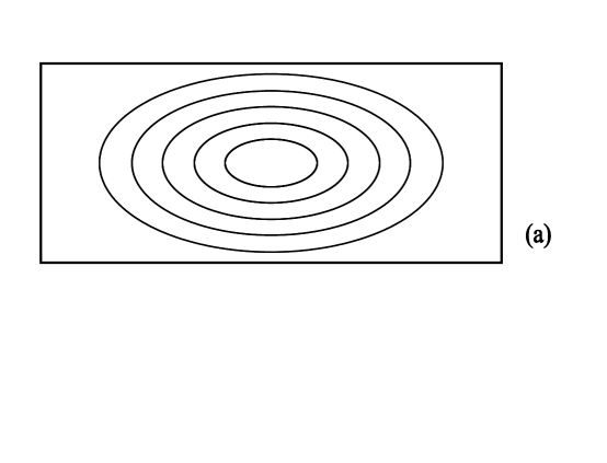
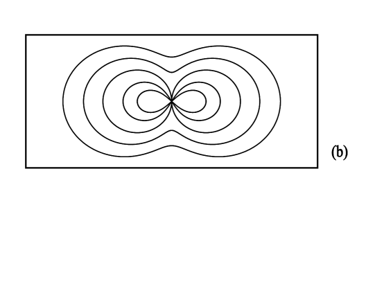
Figure 1: Schematic plot of structure factors. (a) Ellipses for a typical anisotropic Ising model in equilibrium. (b) “Butterfly” or “owl” pattern for a driven system.

Strange as it may seem, this behavior can be understood within the context of the continuum approach, Eqn. (1). For $T\gg T_{c}$, both $\tau_{\|}$ and $\tau_{\bot}$ are positive. Thus, the local magnetization $\varphi({\bf x},t)$ fluctuates around a stable minimum at zero, and neither the fourth-order derivatives nor the nonlinearities are necessary for stability. As a consequence, the behavior of the system in the disordered phase can be described by a much simpler, linear Langevin equation, namely,

$$\partial_{t}\varphi({\bf x},t)=\lambda(\tau_{\bot}\nabla_{\bot}^{2}+\tau_{\|}\partial^{2})\varphi-\nabla{\bf\eta}.$$ (3)

With the help of a Fourier transform, we can easily find $\varphi({\bf k},t)$ for any realization of ${\bf\eta}$, and then compute averages over the Gaussian distributed ${\bf\eta}$, with its second moment given by (1). This forms the starting point for the discussion of the disordered phase, quantified by, e.g., equal-time structure factors or three-point functions [21].

Here, we focus on the former, $S({\bf k})\equiv<\varphi({\bf k},t)\varphi(-{\bf k},t)>$, which can be easily computed:

$$S({\bf k})=\frac{\sigma_{\bot}k_{x}^{2}+\sigma_{\|}k_{y}^{2}}{\tau_{\bot}k_{x}^{2}+\tau_{\|}k_{y}^{2}+O(k_{x}^{4},k_{x}^{2}k_{y}^{2}{\bf,}k_{y}^{4}{\bf)}},$$ (4)

so that $R=\left(\sigma_{\|}\tau_{\bot}\right)/\left(\sigma_{\bot}\tau_{\|}\right)$. In order for this $S$ to reduce to the equilibrium Ornstein-Zernike form, the FDT has to be invoked, which constrains $R$ to unity. For the driven case, $R$ is no longer constrained, so that a discontinuity develops. One consequence of such a singularity in $S$ is that $G$ becomes long-ranged, decaying as ${\bf r}^{-2}$ at large $|{\bf r|}$. The amplitude, in addition to being $\propto(R-1)$, has a dipolar angular dependence, so that an appropriate angular average of $G$ is again short-ranged [6].

To end this discussion, let us follow G. Grinstein’s argument [22] that such long-ranged power law decays should be expected. Starting with the dynamic two-point correlation $G({\bf r},t)$, we know that the conservation law leads to the autocorrelation: $G({\bf 0},t)\rightarrow t^{-d/2}$. In addition, being a diffusive system, we should expect ${\bf r}\sim\sqrt{t}$, at least far from criticality. Using naive scaling, we would write $G({\bf r},0)\rightarrow|{\bf r}|^{-d}$! In other words, the generic behavior of $G$ in a diffusive system is $|{\bf r}|^{-d}$ decay, not exponential. In this case, the equilibrium system is the non-generic one, in which the amplitude of this generic term is forced to vanish, by FDT. Our familiarity with equilibrium systems is so strong that, on first sight, power law decays far above $T_{c}$ appear quite surprising. Finally, note that a scaling argument of this kind cannot produce the angular dependence, a crucial feature of the generic singularities of driven diffusive systems.

3.2 $T$ far below $T_{c}$

Next, we turn to systems far below $T_{c}$. Due to the conservation law, they typically display phase co-existence, so that the dominant fluctuations and slow modes are those associated with the interface between the phases. Again, for the $d=2$ Ising model in equilibrium, there is a wealth of information on the properties of the interface [23]. In particular, being a one-dimensional object, the interface exhibits behavior identical to a simple random walk [18] at the large scales, such as widths diverging as $\sqrt{L}$. In our case, if we study an interface aligned along the $y$ axis, then, to a good approximation, we may specify the configuration by its position along $x$ by the “height” function $h(y)$. Known as capillary waves [24], these fluctuations have a venerable history. Since the interface is a manifestation of broken translational invariance, $h(y)$ are the soft Goldstone modes [17], so that the associated structure factor $S_{h}(q)\equiv\left\langle h(q)h(-q)\right\rangle$ diverges as $q^{-2}$. Of course, this property is just the Fourier version of the $\sqrt{L}$ divergence: $\int_{1/L}q^{-2}dq=O(L)$. Interfaces with divergent widths are also known as “rough”; only for $d>2$ may interfaces in crystalline Ising-like models display transitions from rough to smooth phases.

When driven, however, the interface width appears to approach a finite width at large distances. In particular, for $E=2J$, using lattices up to $L_{y}=60$ and plotting the widths vs. $L^{p}$ with various values of $p$, we found that the curves did not straighten out with $p$ as low as 0.05 [25]. As a phenomenon, roughness suppression is not novel, gravity being the most common example. However, the drive here is parallel to the interface, reminiscent of wind driving across a water surface, which has a destabilizing effect by contrast. Subsequently, a more detailed simulation study [26] of the interface with $L_{y}\leq 600$ showed that $S(q)\sim q^{-2}$ for large $q$, crossing over to $q^{-0.67}$ for small $q$ (Fig. 2). Since $\int_{1/L}q^{-0.67}dq=O(1)$ , the small $q$ behavior is consistent with $p=0$. Though $0.67$ appears temptingly close to a simple rational: $2/3$, there is no viable theory so far (despite two valiant attempts [27]). Finally, let us note that the crossover from rough to smooth occurs at the scale of $q\sim E$. Although no precise Monte Carlo analysis of this crossover has been performed, it is consistent with $E$ having the units of 1/length. In this respect, such a length is comparable to the capillary length which controls the crossover in the gravitationally stabilized interface. Of course, in that case, the small $q$ behavior is simply $q^{0}$!

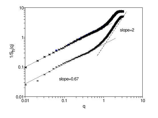
Figure 2: Log-log plot of interface structure factor vs. wavevector.

3.3 Critical Properties

Finally, we turn to the critical region, described by $\tau_{\bot}\gtrsim 0$ in (1). In contrast to the situation for $T\gg T_{c}$, we now need fourth-order terms in $\nabla_{\bot}$ to stabilize the system against large-wavelength fluctuations. Similarly, the nonlinear terms are required to ensure a stable ordered phase below $T_{c}$. However, we still have $\tau_{\|}>0$, so that fourth-order parallel gradients may safely be neglected. Thus, near criticality, the leading terms on the right hand side of (1) are $(\nabla_{\bot}^{2})^{2}\varphi$ and $\partial^{2}\varphi$, implying that parallel and transverse wave vectors, ${\bf k}_{\bot}$ and ${\bf k}_{\|}$, scale naively as $|{\bf k}_{\|}|\sim|{\bf k}_{\bot}|^{2}$, i.e., parallel gradients are less relevant than transverse ones. More systematically, a naive dimensional analysis [28] reveals that the nonlinearity associated with ${\cal E}$ is the most relevant one, having an upper critical dimension $d_{c}=5$, distinct from the usual value of $4$ for the Ising model. Dropping irrelevant terms, (1) simplifies to

$$\partial_{t}\varphi({\bf x},t)=\lambda\{(\tau_{\bot}-\nabla_{\bot}^{2})\nabla_{\bot}^{2}\varphi+\partial^{2}\varphi+\frac{u}{3!}\nabla_{\bot}^{2}\varphi^{3}+{\cal E}\partial\varphi^{2}\}-\nabla_{\bot}{\bf\eta}_{\bot}({\bf x},t)$$ (5)

with noise term ($i,j=1,...,d-1$)

$$<\eta_{\bot i}({\bf x},t)\eta_{\bot j}({\bf x}^{\prime},t^{\prime})>=2\sigma_{\bot}\delta_{ij}\delta(x-x^{\prime})\delta(t-t^{\prime}).$$

Here, we have rescaled $\tau_{\|}$ to $1$ and have kept the (naively irrelevant) nonlinearity associated with $u$, to ensure a stable theory below $T_{c}$. This is the starting point for the analysis of universal critical behavior.

In this regime, large fluctuations on all length scales dominate the behavior of the system, so that renormalization group techniques are indispensable. To summarize very briefly, the Langevin equation (5) is recast as a dynamic functional [29], followed by a renormalized perturbation expansion in $\epsilon\equiv d-d_{c}$ [28]. The quartic coupling $u$ must be treated as a dangerously irrelevant operator. Gratifyingly, the series for the critical exponents can be summed, so that we obtain quantitatively reliable values even in two dimensions. The details are quite technical [30], so that we just review the key results here.

The discussion leading to (5) already suggests that the critical behavior of the driven system is distinct from its equilibrium counterpart: the upper critical dimension is shifted to $d_{c}=5$, and parallel and transverse wave vectors scale with different exponents. Anticipating renormalization, we reformulate their scaling as $|{\bf k}_{\|}|\sim|{\bf k}_{\bot}|^{1+\Delta}$, introducing the strong anisotropy exponent $\Delta$. To illustrate its importance, let us consider the wave vector scaling for the equilibrium Ising model. For isotropic exchange interactions, coarse-graining results in the usual Landau-Ginzburg Hamiltonian with gradient term $(\nabla\varphi)^{2}$. Clearly, this cannot lead to anything but $|{\bf k}_{\|}|\sim|{\bf k}_{\bot}|$. The only effect of anisotropies in the microscopic couplings is to give rise to different amplitudes, so that $\Delta$ remains zero. We refer to this situation as weak anisotropy, in contrast to strong anisotropy where $\Delta\neq 0$. Examples of the latter in equilibrium models include, e.g., Lifshitz points or structural phase transitions [31].

For any system with strong anisotropy, irrespective of its universality class, the renormalization group predicts the general scaling form of, e.g., the dynamic structure factor near criticality:

$$S({\bf k},t;\tau_{\bot})=\mu^{-2+\eta}S(k_{\|}/\mu^{1+\Delta},{\bf k}_{\perp}/\mu,t\mu^{z};\tau_{\perp}/\mu^{1/\nu})$$ (6)

Here, $\mu$ is just a scaling factor. Eqn. (6) can be viewed as a definition of the critical exponents $\nu$, $z$, $\eta$ and $\Delta$. The appearance of the latter is of course consistent with our earlier discussion. Different universality classes are distinguished by the characteristic values of these exponents, expressed, e.g., through their $\epsilon$-expansions. For our model, all exponents, except $\Delta$, take their mean-field values: $\nu=\frac{1}{2}$, $z=4$, $\eta=0$ while $\Delta=1+\frac{\epsilon}{3}$. A separate analysis yields the order parameter exponent $\beta=\frac{1}{2}$. Note that all of these equalities are exact, i.e., all higher order terms in the $\epsilon$-expansion vanish!

Care must be taken on two fronts, both associated with the presence of strong anisotropy, when comparing these exponents to Monte Carlo data. First, in the equilibrium Ising model, the same exponent $\eta$ characterizes the divergence of the critical structure factor near the origin in ${\bf k}$-space, $S({\bf k},t=0;\tau_{\perp}=0)\sim|{\bf k}|^{-(2-\eta)}$ for ${\bf k}\rightarrow 0$, and the power law decay of its Fourier transform, the two-point correlations, $G({\bf r},t=0;\tau_{\perp}=0)\sim|{\bf r}|^{-(d-2+\eta)}$ as $|{\bf r}|\rightarrow\infty$. In contrast, four $\eta$-like exponents are needed in the driven case! Fortunately, scaling laws relate them to $\eta$ and $\Delta$. For example, we can define $\eta_{\bot}$ via $S(k_{\|}=0,{\bf k}_{\perp},t=0;\tau_{\perp}=0)\sim|{\bf k}_{\perp}|^{-(2-\eta_{\bot})}$, for $|{\bf k}_{\perp}|\rightarrow 0$. Using (6), we read off the simple result $\eta_{\bot}=\eta$. Similarly, we introduce $\eta_{\|}^{\prime}$ through the relation $G(r_{\|},{\bf r}_{\bot}={\bf 0},t=0;\tau_{\perp}=0)\sim r_{\|}^{-(d-2+\eta_{\|}^{\prime})}$, for $r_{\|}\rightarrow\infty$. Keeping track of $\Delta$ in the Fourier transform, we obtain the less trivial scaling law $\eta_{\|}^{\prime}=\frac{\eta-\Delta(d-3)}{1+\Delta}$. Since most simulations have focused on two-dimensional systems, we set $\epsilon=3$, predicting $\Delta=2$ and $\eta_{\|}^{\prime}=2/3$. Monte Carlo data for the pair correlation along the drive beautifully display the expected $r_{\|}^{-2/3}$ decay [32]. Numerical evidence for the strong anisotropy exponent is somewhat more indirect, extracted from an anisotropic finite size scaling analysis [7]. Convincing data collapse is obtained, using anisotropic systems of size $L_{\|}\times L_{\bot}$ with fixed “aspect” ratio $L_{\|}/L_{\bot}^{1+\Delta}$, for the theoretically predicted values of the exponents.

It is intriguing that the signals of continuous phase transitions in or near equilibrium, namely, a diverging length scale, scale invariance and universal behavior, also mark such transitions in far-from-equilibrium scenarios.

4 Some Recent Developments

Beyond the topics discussed in the previous section, we may arbitrarily name three other “levels” of non-equilibrium steady-state systems. The first are associated with the KLS model itself, including fascinating results on higher correlations [21], failure of the Cahn-Hilliard approach to coarsening dynamics [33], models with shifted periodic and/or open boundary conditions [34], and systems with AC or random drives [35, 16]. Topics in the next “level” involve various generalizations of KLS, such as other interactions [36, 37], multi-layer systems, multi-species models, and systems with quenched impurities [38]. Further “afield” is a wide range of driven systems, e.g., surface growth, electrophoresis and sedimentation, granular and traffic flow, biological and geological systems, etc. In these brief lecture notes, we present two topics at the “intermediate level”: a driven bi-layer system and a model with two species.

4.1 Phase Transitions in a Bi-layer Lattice Gas

The physical motivation for considering multi-layered systems may be traced to intercalated compounds [39]. The process of intercalation, where foreign atoms diffuse into a layered host material, is well suited for modeling by a driven lattice gas of several layers. In both physical systems and Monte Carlo simulations of a model with realistic parameters [40], finger formation has been observed. Both are transient phenomena, so that we might ask: are there any novel phenomena in the driven steady states? On the theoretical front, there are two motivations. To study critical behavior of the single layer KLS model, it is necessary to set the overall density at 1/2, with the consequence that two interfaces develop below criticality. These interfaces seriously complicate the analysis, since their critical behavior is quite distinct from the bulk. One way to avoid these difficulties is to consider a bi-layer system [41], with no inter-layer interactions. Through particle exchange between the layers, the system may order into a dense and a hole-rich layer, neither of which has interfaces. Certainly, this is expected (and observed) in the equilibrium case, where the steady state is just two Ising models, decoupled except for the overall conservation law. The other is using multilayer models as “interpolations” from two- to three-dimensional systems [42]. Motivations aside, what the simulations reveal is entirely unexpected.

In the simplest generalization, a bi-layer system is considered as a fully periodic $L\times L\times 2$ model. The first simulations were carried out on the case with zero inter-layer interactions [42]. Therefore, within each layer, all aspects are identical to the KLS model. Particle exchanges across the layers, unaffected by the drive, are updated according to the local energetics alone, so that these jump rates are identical to a system in equilibrium. The overall particle density is fixed at 1/2. In the absence of $E$, there would be a single second order transition at the Onsager temperature. Since the inter-layer coupling is zero, phase segregation at low temperatures will occur across the layers, i.e., the ordered phase is characterized by homogeneous layers of different densities (opposite magnetizations, in spin language). Having no interfaces, the free energy of the system is clearly lowest in such a state. At $T=0$, one layer will be full and the other empty, so that this state will be labeled by FE.

Intriguingly, when $E$ is turned on, two transitions appear [42]! As $T$ is lowered, the homogeneous, disordered (D) phase first gives way to a state with strips in both layers, reminiscent of two entirely unrelated, yet aligned, single layer driven systems. We will refer to this state as the strip phase (S). As $T$ is lowered further, a first order transition takes the S phase into the FE state. Why the S state should interpose between the D and FE states was not understood. This puzzle, together with the presence of interlayer couplings in intercalated compounds, motivated our study of the interacting bi-layer driven system [43]. Within this wider context, the presence of two transitions is no longer a total mystery. On the other hand, this study reveals several unexpected features, leading to interesting new questions.

Our system consists of two $L^{2}$ Ising models with attractive interparticle interactions of strength unity. Arranged in a bi-layer structure, the inter-layer interaction is specified by $J$. Thus, the “internal” Hamiltonian is just ${\cal H}\equiv-4\sum nn^{\prime}-4J\sum nn^{\prime\prime},$ where the first sum is over nearest neighbors within a given layer while $n$ and $n^{\prime\prime}$ differ only by the layer index. The external drive, $E$, is imposed through the jump rates, as in Section II. For simulations, we kept the overall density at 1/2 and chose $J\in$ $[-10,10]$. Note that negative $J$’s are especially appropriate for intercalated materials [39, 40]. The eventual goal of such a study is to map out the phase diagram in the $T$-$J$-$E$ space. So far, we have data for only three (positive) values of $E$. Not expecting further surprises, we believe that we have uncovered the main features of the phase diagram.

To begin, let us point out various features in the equilibrium case. Here, the $J>0$ and the $J<0$ systems can be mapped into each other by a gauge transformation. Thus, in the thermodynamic limit, the phase diagram in the $T$-$J$ plane is exactly symmetric. However, for the lattice gas constrained by a conservation law, the low temperature states of these two systems are not the same, being S or FE, respectively. While the D-S or D-FE transitions are second order (shown as a line in Fig. 3), the S-FE line will be first order in nature ($T$ axis from 0 to 1 in Fig. 3). Due to the presence of interfaces, the FE domain includes the $J\equiv 0$ line. For the same reason, it “intrudes” into the $J>0$ half plane by $O(1/L)$, for finite systems. Of course, on the $T$ axis lies a pair of decoupled Ising systems, so that $T_{c}(J$=$0)$ assumes the Onsager value, as $L\to\infty$. In general, $T_{c}(J)$ is not known exactly, though $T_{c}(J$=$\pm\infty)$ is precisely $2T_{c}(J$=$0)$, since every configuration of the two layers can be mapped into one in the usual Ising model. The lesson from equilibrium is now clear: the S state is as generic as the FE state in this wider context. As we will see below, the presence of two transitions does not represent a qualitative change from the equilibrium phase structure.

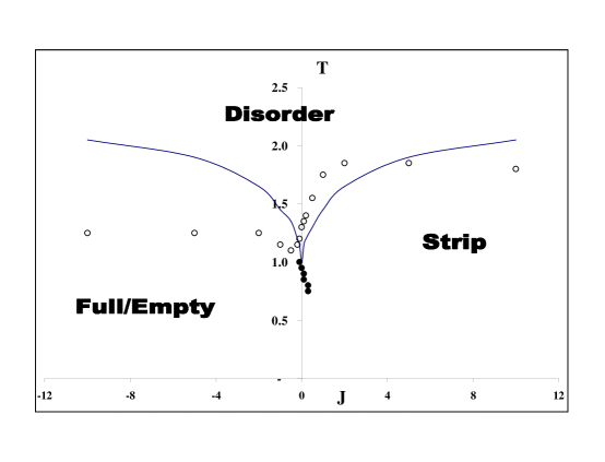
Figure 3: Phase diagrams for the bi-layer Ising lattice gas. Solid lines are second order transitions in the equilibrium case. Open/solid circles are continuous/discontinous transitions in the driven case.

Turning to driven systems, we can no longer expect a symmetric phase diagram, since the drive breaks the Ising symmetry. The data for $E=25$ are shown in Fig. 3, in which the first/second order transitions are marked as solid/open circles. We see that the only effect of the drive is to shift the phase boundaries. No new phases appear while the nature of the transitions remains unchanged. However, there are remarkable features. One is the lowering of the critical temperature for large $\mid\!J\mid$. Given that $T_{c}(E)>T_{c}(0)$ in the KLS model, it is quite unexpected that $T_{c}(|J|\gg 1,E\gg 1)$ is less than its equilibrium counterpart. Perhaps more notable is the presence of a small region in the $J<0$ half plane, in which an S-phase is stable. Since particle-rich strips lie on top of each other, such a phase could not exist if either energy or entropy were to dominate the steady state. Concerned that its presence might be a finite size effect, we performed simulations using $L$’s up to $100$, with $J=-0.1$ and $T\in[1.00,1.20]$. In all cases, the S-phase prevailed, leading us to conjecture that this region exists even in the thermodynamic limit. On the other hand, for lower $T$, the FE-phase penetrates into the $J>0$ half plane, as in equilibrium cases. Energetics seem to take the upper hand here. Though we believe that, as $L\to\infty$, this part of the phase boundary will collapse onto the $J=0$ line, we have not checked the finite size effects explicitly. Of course, these “intrusions” into the positive/negative $J$ region by the FE/S-phase are responsible for the appearance of two transitions in the studies of the $J\equiv 0$ model [42].

It would clearly be useful to develop some intuitive arguments which can “predict” these qualitative modification of the equilibrium phase structure. Since the usual energy-entropy considerations appear to fail, our attempt [43] is based on the competition between suppression of short-range correlations [44] and enhancement of long-range ones [32], as a result of driving. Let us focus on the two-point correlations in the disordered phase with $T$ being lowered from $\infty$ and see how they are affected by the drive. On the one hand, the nearest-neighbor correlations are found to be suppressed by $E$, consistent with the picture that the drive acts as an extra noise in breaking bonds. Taken alone, this suppression would lead to the lowering of the critical temperature, as pointed out in Section II. On the other hand, as we showed above, the drive changes significantly the large distance behavior of $G$, from an exponential to a power law. Further, the amplitude is positive (negative) for correlations parallel (transverse) to $E$. Both the positive longitudinal correlations and the negative transverse ones should help the process of ordering into strips parallel to the field. In other words, the enhanced long-range parts favor the S-phase. Taken alone, we expect this effect to increase $T_{c}(E)$. Evidently, for the single layer case, the latter effect “wins”. For a bi-layer system, we need to take into account cross-layer correlations, which are necessarily short-ranged.

Focusing first on the $J=0$ case, where short-range effects due to cross-layer interactions are absent, we are led to $T_{c}(0,E)/T_{c}(0,0)>1$. Indeed, this ratio is comparable to that in the single-layer case. Next, we consider systems with positive $J$. Without the drive, $T_{c}(J,0)$ is of course enhanced over $T_{c}(0,0)$. For non-vanishing drive, it is not possible to track the competition between the short- and long-range properties of the transverse correlations. Evidently, for small $J$, the long-range part still dominates, so that $T_{c}(J,E)/T_{c}(J,0)>1.$ However, for $J\gg J_{0}$ , the presence of $E$ effectively lowers $J$, since the latter is associated with only short-range correlations. Since a lower effective $J$ naturally gives rise to a lower $T_{c}$ , we would “predict” that $T_{c}(J,E)/T_{c}(J,0)$ could decrease considerably as $J$ increases. From Fig.3, we see that $T_{c}(J,E)<T_{c}(J,0)$ for $J\geq 5!$ The interplay of the competing effects is so subtle that either can dominate, in different regions of the phase diagram. Finally, we turn to the $J<0$ case. Here, the two effects tend to co-operate rather than compete, since the long-range parts favor the S-phase over the FE-phase. As a result, the domain of FE is smaller everywhere. In particular, note that the $J<0$ branch of $T_{c}(J,E)$ is significantly lower than the $J>0$ branch. The small region of the S-phase can be similarly understood, at least at the qualitative level. In this picture, we may argue that the bicritical point and its trailing first order line should be “driven” to the $J<0$ half-plane.

To end this subsection, we point out a few other interesting features. The order parameters of the S and FE phases are conserved and non-conserved, respectively. Based on symmetry arguments, we may expect that the critical properties of the two second order branches will fall into different universality classes. In contrast, the gauge symmetry forces static equilibrium properties to be identical along these two branches [45]. Since the drive breaks this symmetry, we can only speculate that the D-S transitions belong to the same class as the single layer, KLS model [30] while the D-FE ones should remain in the equilibrium Ising class [14]. Since these two classes are distinct, we can also expect a rich crossover structure near the bi-critical point. Assuming these conjectures are confirmed, we can truly marvel at the novelties a driving field can bring.

4.2 Biased Diffusion of Two Species

If the particles in the KLS model are considered “charged”, it is natural to explore the effects of having both positive and negative charges. Defined on a fully periodic $L_{x}\times L_{y}$ square lattice, a configuration of such a “two species” model can be characterized by two local occupation variables, $n_{{\bf r}}^{+}$ and $n_{{\bf r}}^{-}$, which equal $1$ ($0$), if a positive or negative particle is present (absent) at site ${\bf r\equiv}(x,y)$. In spin language, this corresponds to a spin-$1$ model, and novel behavior is to be expected, since we have altered the internal symmetries of the local order parameter. For simplicity, we will restrict ourselves to zero total charge, $Q\equiv\sum_{{\bf r}}(n_{{\bf r}}^{+}-n_{{\bf r}}^{-})=0$. Pursuing the analogy to electric charges, positive (negative) charges move preferentially along (against) the drive $E$ which is directed along the $-y$ axis. As a first step, we assume that there are no interparticle interactions apart from an excluded volume constraint. Thus, our model can be viewed as the high-temperature, large $E$ limit of a more complicated interacting system. To model biased diffusion, a particle with charge $q=\pm 1$ jumps onto a nearest-neighbor empty site according to $\min[1,e^{-qE\,\delta y}]$, where $\delta y=0,\pm 1$ is the change in the $y$-coordinate of the particle. To allow charge exchange between neighboring particles, two nearest-neighbor sites carrying opposite charge may exchange their content with probability $\gamma\min[1,e^{-qE\,\delta y}]$. Now, $\delta y$ is the change in the $y$-coordinate of the positive particle. The parameter $\gamma$ sets the ratio of the characteristic time scales controlling, respectively, charge exchange and diffusion.

Physical motivations for this model come from various directions: fast ionic conductors with several species of mobile charges [1], electric breakdown of water-in-oil microemulsions [46], and gel electrophoresis of charged polymers [47]. It can also be interpreted as a simple model for some traffic or granular flows [48, 49].

Summarizing our simulation data, we first map out the phase diagram of the model, in the space spanned by $E$, the total mass density $\bar{m}\equiv\sum_{{\bf r}}(n_{{\bf r}}^{+}+n_{{\bf r}}^{-})/(L_{x}L_{y})$, and $\gamma$ [50]. Focusing on small $\gamma$, the diffusive dynamics is limited by the excluded volume constraint. For sufficiently small $E$ and $\bar{m}$, typical configurations are disordered, characterized by homogeneous charge and mass densities and fairly large currents. Nevertheless, this phase is highly nontrivial, supporting anomalous two-point correlations reminiscent of the KLS model: In generic directions, the familiar $r^{-d}$ decay prevails, with the remarkable exception of the field direction, where a novel $r_{\|}^{-(d+1)/2}$ dominates [51]. With increasing $E$ or $\bar{m}$, the tendency of the particles to impede one another becomes more pronounced, until a phase transition into a spatially inhomogeneous “ordered” phase occurs. Beyond the transition line $E_{c}($ $\bar{m},\gamma)$, typical configurations are charge-segregated, consisting of a strip of mostly positive charges “floating” on a similar strip of negative charges, surrounded by a background of holes.

To explore these transitions more quantitatively, we need to define a suitable order parameter. Taking the Fourier transforms of the local hole and charge densities, $\tilde{\phi}(k_{\bot},k_{\|})\equiv\frac{1}{L_{x}L_{y}}\sum_{{\bf r}}[1-(n_{{\bf r}}^{+}+n_{{\bf r}}^{-})]\exp\{ik_{\bot}x+ik_{\|}y\}$ and $\tilde{\psi}(k_{\bot},k_{\|})\equiv\frac{1}{L_{x}L_{y}}\sum_{{\bf r}}[n_{{\bf r}}^{+}-n_{{\bf r}}^{-}]\exp\{ik_{\bot}x+ik_{\|}y\}$, we select the components $\Phi\equiv|\tilde{\phi}(0,\frac{2\pi}{L_{y}})|$ and $\Psi\equiv|\tilde{\psi}(0,\frac{2\pi}{L_{y}})|$ since these are most sensitive to ordering into a single transverse strip. Naturally, we choose their averages $<\Phi>$ and $<\Psi>$ as our order parameters. To distinguish first from second order transitions, we also measure their fluctuations and histograms. The resulting phase diagram is shown in Fig. 4. Typically, hysteresis loops in $<\Phi>$ , $<\Psi>$ and the average current are observed only for $\bar{m}<\bar{m}_{o}(\gamma)$, indicating that the transitions are first order in this regime. On the other hand, fluctuations develop sharp peaks for larger mass densities, signalling continuous transitions. Larger values of $\gamma$ favor the disordered phase, so that the whole transition line shifts to higher $E$, the region between the spinodals narrows, and $\bar{m}_{o}(\gamma)$ moves to higher mass densities. Thus, we observe a surface of first order transitions, separated from a surface of continuous ones by a line of multicritical points: $E_{c}(\bar{m}_{o}(\gamma),\gamma)$.

Figure 4: Phase diagram for the driven two-species model. The system size is $30\times 30$. The filled circles mark the lines of continuous transitions, while the open circles denote the spinodal lines associated with first order transitions. The inset shows a typical ordered configuration at $\bar{m}=0.40$, $E=3.00$ and $\gamma=0.02$ with the open (filled) circles representing positive (negative) charges.

While it is not surprising that the disordered phase is stable for large $E$ provided the mass density is sufficiently small, it may appear rather counterintuitive that it should also dominate the $\bar{m}\lesssim 1$ region. However, setting $\bar{m}\equiv 1$ eliminates every hole in the system so that the dynamics is carried entirely by the charge exchange mechanism. Relabelling positive charges as “particles” and negative ones as “holes”, the model becomes equivalent to a noninteracting (i.e., $J=0$) KLS model. Also termed the asymmetric simple exclusion process (ASEP) in the literature, its steady-state solution is exactly known [52] to be homogeneous. Thus, for all $\gamma>0$, our two-species model remains disordered along the entire $\bar{m}\equiv 1$ line. For sufficiently large $\gamma$, the data indicate quite clearly that a finite region of disorder persists, for any $E$, just below complete filling. For smaller $\gamma$, however, it is less obvious whether such a region exists in the thermodynamic limit, since even a single hole can suffice to induce spatial inhomogeneities in a finite system: Acting as a catalyst for the charge segregation process, the hole creates a strip of predominantly positive charge, separated by a rather sharp interface from a similar, negatively charged domain, located “downstream”. The charge exchange mechanism tends to remix the charges but has little effect for small $\gamma$. Eventually, the hole ends up trapped in the interfacial region! Finally, we turn to larger values of $\gamma$, specifically, $\gamma\gtrsim 0.62$: here, the charge exchange mechanism dominates over the excluded volume constraint and suppresses the ordered phase completely.

So far, our discussion has mostly drawn upon Monte Carlo results. It is gratifying, however, that the same qualitative picture emerges from a mean-field theory, based upon a set of equations of motion for the local densities. We briefly summarize the analytic route. Since the numbers of both positive and negative charges are conserved, we begin with a continuity equation for the coarse-grained densities $\rho^{\pm}({\bf r},t)$: $\partial_{t}\rho^{\pm}+\nabla{\bf j}^{\pm}=0$. For simplicity, we focus on the case $\gamma=0$, i.e., particle-hole exchanges, first. As for the KLS model, ${\bf j}^{\pm}$ can be written as the sum of a diffusive piece and an Ohmic term, ${\bf j}^{\pm}=\lambda^{\pm}\{-\nabla\frac{\delta{\cal H}}{\delta\rho^{\pm}}_{|\rho^{\mp}}\pm{\cal E}{\bf\hat{y}}\}$. The density-dependent mobility $\lambda^{\pm}$ must vanish with both $\rho^{\pm}$ and the local hole density, $\varphi\equiv 1-(\rho^{+}+\rho^{-})$, i.e., $\lambda^{\pm}=\rho^{\pm}\varphi$. The “Hamiltonian” ${\cal H}=\{\rho^{+}\ln\rho^{+}+\rho^{-}\ln\rho^{-}+\varphi\ln\varphi\}$ is just the mixing entropy associated with distributing $L_{x}L_{y}\rho^{+}$ positive and $L_{x}L_{y}\rho^{-}$ negative charges over a lattice of $L_{x}L_{y}$ sites. Note that the functional derivative $\frac{\delta{\cal H}}{\delta\rho^{\pm}}$ is taken at fixed $\rho^{\mp}$ since we are focusing on particle-hole exchanges here. To model the charge exchange mechanism, we simply add a similar term to ${\bf j}^{\pm}$, namely, ${\bf j}^{\pm}=\lambda\{-\nabla\frac{\delta{\cal H}}{\delta\rho^{\pm}}\pm{\cal E}{\bf\hat{y}}\}+\gamma\lambda^{\prime}\{-\nabla\frac{\delta{\cal H}}{\delta\rho^{\pm}}_{|\varphi}\pm{\cal E}{\bf\hat{y}}\}$ where $\lambda^{\prime}=\rho^{+}\rho^{-}$ vanishes with both $\rho^{+}$ and $\rho^{-}$, and the functional derivative is taken at fixed hole density. Expressing the resulting equations in the more convenient variables $\varphi$ and charge density $\psi\equiv\rho^{+}-\rho^{-}$, we obtain

$$\partial_{t}\varphi = \nabla\{\nabla\varphi+{\cal E}\varphi\psi{\bf\hat{y}}\}$$

$$\partial_{t}\psi = \nabla\{\gamma\nabla\psi+(1-\gamma)[\varphi\nabla\psi-\psi\nabla\varphi]-{\cal E}\varphi(1-\varphi){\bf\hat{y}}$$

$$-\frac{\gamma}{2}{\cal E}[(1-\varphi)^{2}-\psi^{2}]{\bf\hat{y}}\}$$

These equations have to be supplemented by periodic boundary conditions and constraints on total mass and charge, $(1-\bar{m})L_{x}L_{y}=\int d^{d}r\varphi({\bf r},t)$ and $0=\int d^{d}r\psi({\bf r},t)$. Also, to be precise, all Laplacians $\nabla^{2}$ should be given the appropriate anisotropic interpretation.

Using (4.2) as our starting point, we seek to recapture the major features of the phase diagram. First, the presence of two phases, uniform vs. spatially structured, is reflected in the existence of both homogeneous and inhomogeneous steady-state solutions of (4.2). The existence of the former is evident, due to the conservation law. Anticipating homogeneity in the transverse directions, we seek the latter in the form $\varphi(y)$, $\psi(y)$. Integrating (4.2) once, the stationary mass and charge currents appear as natural integration constants. Since the numbers of positive and negative charges are equal, the former must be zero, leaving us with the latter: $J$. The first equation allows us to eliminate $\psi$ in favor of $\varphi$, and, with $u\equiv\sqrt{1+\frac{\gamma}{(1-\gamma)\varphi}}$ as the new variable, we can reduce the second equation to potential form, $u^{\prime\prime}=-\frac{dV(u)}{du}$. The potential $V(u)$, given explicitly in [50], exhibits a minimum for a range of $J$’s, so that inhomogeneous, periodic solutions of (4.2) exist. We note in passing that these may even be found explicitly, provided $\gamma=0$ [53]. Otherwise, numerical integration is of course always possible, yielding rather impressive agreement with simulation profiles. Interestingly, our equations of motion predict that ${\cal E}$ enters only through the scaling variable ${\cal E}L_{y}$. If plotted accordingly, our simulation data confirm this scaling by collapsing rather convincingly, at least within their error bars.

However, the mere existence of two types of steady-state solutions is not sufficient to provide evidence for a phase transition. Therefore, we seek instabilities of these solutions, as the control parameters ${\cal E}$, $\bar{m}$ and $\gamma$ are varied. Performing a linear stability analysis, we find that a homogeneous solution with mass $\bar{m}$ becomes unstable if the drive ${\cal E}$ exceeds a threshold value ${\cal E}_{H}(\bar{m},\gamma)=\frac{2\pi}{L_{y}}\sqrt{\frac{1-\bar{m}+\gamma\bar{m}}{(1-\bar{m})[(2-\gamma)\bar{m}-1]}}$. The most relevant perturbation is associated with the smallest wave vector in the parallel direction, $({\bf 0,}2\pi/L_{y})$. A simple analysis of ${\cal E}_{H}(\bar{m},\gamma)$ shows that this instability can only occur within the interval $\frac{1}{2-\gamma}<\bar{m}<1$, so that, in particular, the homogeneous phase is always stable for $\gamma\geqslant 1$. Clearly, we cannot identify this mean-field stability boundary with the true transition line: we have not considered the locus of instabilities associated with inhomogeneous solutions, and fluctuations have been neglected throughout. However, it is quite remarkable how well it mirrors the qualitative shape of the phase diagram.

Finally, let us consider the order of the transitions. In principle, two routes can be pursued here. One of these, namely, the computation of the stability boundary of the inhomogeneous phase, ${\cal E}_{I}(\bar{m},\gamma)$, is rather subtle, involving three Goldstone modes [54]. Once ${\cal E}_{I}(\bar{m},\gamma)$ is known, values $(\bar{m},\gamma)$ for which ${\cal E}_{I}$ and ${\cal E}_{H}$ coincide can be identified as loci of continuous transitions; otherwise, ${\cal E}_{H}$ and ${\cal E}_{I}$ mark the “spinodals”, near a first order transition, where the homogeneous/inhomogeneous phases become linearly unstable. Alternatively, the adiabatic elimination of the fast modes results in an effective equation of motion for the slow ones which can then be analyzed. Since the technical details of this approach can be found in [50], we need only focus on the result which combines the expected with the surprising. Letting $M(q_{\bot},t)$ denote the complex amplitude of the unique slow mode, associated with the band of wave vectors $(q_{\bot}{\bf,}2\pi/L_{y})$, its equation of motion takes the Ginzburg-Landau form: $\partial_{t}M=-\{(\tau+q_{\bot}^{2})M+gM|M|^{2}+O(M^{5})\}$. Here, $\tau$ is the soft eigenvalue, which vanishes on the stability boundary and $g=g({\cal E},\bar{m},\gamma,L_{y})$ is a rather complicated function. As in standard Landau theory, the sign of $g$ determines the order of the transition: if positive, the transition is continuous while negative $g$ signals a first order one. Since $\tau\simeq 0$, we can set ${\cal E}={\cal E}_{H}$ and discuss $g$ on the stability boundary itself: being positive for $\bar{m}\lesssim 1$, it has a unique zero at a critical $\bar{m}_{o}(\gamma)$, below which it becomes negative. Since $\bar{m}_{o}(\gamma)$ increases with $\gamma$, we recover the qualitative behavior of the multicritical line observed in the simulations. The surprising aspect of this equation of motion, however, resides in the fact that $M$ is O(2)-symmetric and $q_{\bot}$ spans just a single spatial dimension. Given these symmetries, the Mermin-Wagner theorem [55] should forbid the existence of long-range order! One might hope that a careful analysis of finite-size effects in this system would contribute to the disentanglement of this puzzle.

We conclude with two comments. First, we noted earlier that the case $\bar{m}\equiv 1$ is exactly soluble. There are, in fact, two other surfaces in the phase diagram, corresponding to $\gamma=1$ and $\gamma=2$, for which certain distributions are exactly known. Setting $\gamma=1$ implies that the rates for particle-hole and particle-particle exchanges become equal, so that any given particle, e.g., a positive charge, cannot distinguish between negative charges and holes. Thus, it experiences biased diffusion, equivalent to the non-interacting KLS model. Accordingly, the marginal steady-state distribution of the occupation numbers of one species is uniform, i.e., $P\left[\{n_{{\bf r}}^{\pm}\}\right]=\sum_{\{n_{{\bf r}}^{\mp}\}}P\left[\{n_{{\bf r}}^{+},n_{{\bf r}}^{-}\}\right]\propto 1$, and observables pertaining to a single species are trivial. For example, the two-point correlation functions for equal charges, $<n_{{\bf r}}^{+}n_{{\bf 0}}^{+}>$ and $<n_{{\bf r}}^{-}n_{{\bf 0}}^{-}>$, vanish for ${\bf r\neq 0}$. The full distribution, $P\left[\{n_{{\bf r}}^{+},n_{{\bf r}}^{-}\}\right]$, however, is nontrivial, so that, e.g., the two-point function for opposite charges, $<n_{{\bf r}}^{+}n_{{\bf 0}}^{-}>$, remains long-ranged [51]. A completely random system, marked by a uniform $P\left[\{n_{{\bf r}}^{+},n_{{\bf r}}^{-}\}\right]$ results only if $\gamma=2$. Finally, we note that the one-dimensional version of our model is exactly soluble by matrix methods [56].

Second, it is natural to wonder about the consequences of having non-zero charge. This problem has only been investigated for $\gamma=0$ [57], but the findings are quite remarkable. The system still orders into a charge-segregated strip, while supporting a nonvanishing mass current, reflected in an overall drift. If, e.g., positive charges outnumber negative ones, one might expect that the whole strip would drift in the field direction - in analogy with American football, where the team with fewer players tends to lose ground. In contrast, the strip wanders against the field, following the preferred direction of the minority charge!

We should add that this model possesses several other intriguing properties, e.g., stable configurations with nontrivial winding number (“barber poles”) [58] or multiple-valued currents in the mean-field description [53]. To summarize, the remarkable richness of this deceptively simple system is clearly amazing.

5 Summary and Outlook

We have presented, within the limited scope of these lecture notes, a brief introduction to the statistical mechanics of driven diffusive systems and some recent developments in this ever expanding field. Focusing only on the prototype model and two of the simplest generalizations, we pointed out a multitude of surprises, when we base our expectations on the experience with equilibrium systems. While some of these, e.g., the generic presence of singular correlations, are rather well understood, others, such as the nature of ordering in two-species models, remain unresolved. Of course, the holy grail of this whole field, namely, the fundamental understanding and theoretical classification of non-equilibrium steady states, still beckons at the distant horizon.

6 Acknowledgments

It is a pleasure to especially acknowledge our collaborators on the recent work reported here: C.C. Hill, G. Korniss and K.-t Leung. Others are too numerous to mention but no less deserving. We thank the IXth International Summer School on Fundamental Problems in Statistical Mechanics, and particularly H.K. Janssen and L. Schäfer, for their hospitality. This research was supported in part by grants from NATO, the SFB 237 of the Deutsche Forschungsgemeinschaft and the US National Science Foundation through the Division of Materials Research.

References

- [1] See, e.g., S. Chandra, Superionic Solids. Principles and Applications (North Holland, Amsterdam 1981).
- [2] S. Katz, J. L. Lebowitz and H. Spohn, Phys. Rev. B 28, 1655 (1983); J. Stat. Phys 34, 497 (1984).
- [3] Ising, Z. Physik 31, 253 (1925). A more recent treatment is, e.g., B. M. McCoy and T. T. Wu, The Two-dimensional Ising Model (Harvard Univ. Press, Cambridge, Mass., 1973).
- [4] C.N. Yang and T.D. Lee, Phys. Rev. 87, 404 (1952); and T.D. Lee and C.N. Yang, Phys. Rev. 87, 410 (1952).
- [5] In particular, see the lithograph Ascending and Descending, reproduced on the cover of [6].
- [6] B. Schmittmann and R. K. P. Zia, Phase Transitions and Critical Phenomena, Vol. 17, edited by C. Domb and J. L. Lebowitz (Academic, London, 1995).
- [7] K.-t. Leung, Phys. Rev. Lett. 66, 453 (1991) and Int. J. Mod. Phys. C3, 367 (1992); J. S. Wang, J. Stat. Phys., 82, 1409 (1996).
- [8] G.L. Eyink, J.L. Lebowitz and H. Spohn, Journal of Statistical Physics 83, 385-472 (1996).
- [9] P.C. Hohenberg and B.I. Halperin, Rev. Mod. Phys. 49, 435 (1977).
- [10] See, e.g., H. Risken, The Fokker-Planck Equation (Springer, Heidelberg 1989).
- [11] H.K. Janssen, in Dynamical Critical Phenomena and Related Topics, ed. C.P. Enz, Lecture Notes in Physics, Vol. 104 (Springer, Heidelberg, 1979).
- [12] The easiest way to see the connection between , and is to recast the Langevin equation in terms of its equivalent Fokker-Planck equation. See Ref. [10].
- [13] R. Kubo, Rep. Progr. Phys. 29, 255 (1966). See R. Graham, Z. Phys. 26 397 (1977) and B40, 149 (1980), for a much deeper discussion of this fundamental issue.
- [14] G. Grinstein, C. Jayaprakash and Y. He, Physical Review Letters 55, 2527 (1985).
- [15] H.K. Janssen and B. Schmittmann, Z. Phys. B63, 517 (1986); R.K.P. Zia and B. Schmittmann, Z. Phys. B97, 327 (1995).
- [16] B. Schmittmann, Europhys. Lett. 24, 109 (1993).
- [17] J. Goldstone, Nuovo Cim., 19, 154, (1961) and H. Wagner, Z. Physik, 195, 273 (1966).
- [18] H. N. V. Temperley, Proc. Cam. Phil. Soc., 48, 683 (1952) and K. Y. Lin and F. Y. Wu, Z. Physik, B33, 181 (1970).
- [19] K.G. Wilson, Rev. Mod. Phys. 47C, 773 (1975). See also Ref. [28].
- [20] L. Onsager, Phys. Rev. 65, 117 (1944) and Nuovo Cim. 6, (Suppl.) 261 (1949).
- [21] K. Hwang, B. Schmittmann and R. K. P. Zia, Phys. Rev. Lett. 67, 326 (1991) and Phys. Rev. E48, 800 (1993).
- [22] G. Grinstein, J. Appl. Phys. 69, 5441 (1991).
- [23] See references in, e.g., R.K.P. Zia, in Statistical and Particle Physics: Common Problems and Techniques, eds. K.C. Bowler and A.J. McKane (SUSSP Publications, Edinburgh, 1984).
- [24] F. P. Buff, R. A. Lovett and F. H. Stillinger, Phys. Rev. Lett., 15, 621 (1965). B. Widom and J.S. Rowlinson, Molecular Theory of Capillarity(Oxford, 1982).
- [25] K.-t. Leung, K. K. Mon, J. L. Vallés and R. K. P. Zia, Phys. Rev. Lett. 61, 1744 (1988) and Phys. Rev. B39, 9312 (1989) ;
- [26] K.-t. Leung and R. K. P. Zia, J. Phys. A26, L737(1993).
- [27] K-t. Leung, J. Stat. Phys. 50, 405 (1988) and 61, 341 (1990); C. Yeung, J.L. Mozos, A. Hernandez-Machado, D. Jasnow, J. Stat. Phys. 70. 1149 (1992).
- [28] D.J. Amit, Field Theory, the Renormalization Group and Critical Phenomena, 2nd revised edition, (World Scientific, Singapore, 1984); J. Zinn-Justin, Quantum Field Theory and Critical Phenomena, (Oxford University Press, Oxford, 1989).
- [29] H.K. Janssen, Z. Phys. B23, 377 (1976); C. de Dominicis, J. Phys. (Paris) Colloq. 37, C247 (1976).
- [30] H.K. Janssen and B. Schmittmann, Z. Phys. B64, 503 (1986); K-t. Leung and J.L. Cardy, J. Stat. Phys. 44, 567 and 45, 1087 (Erratum) (1986).
- [31] R.M. Hornreich, M. Luban, and S. Shtrikman, Phys. Rev. Lett. 35, 1678 (1975); R.A. Cowley, Adv. Phys. 29, 1 (1980); A.D. Bruce, Adv. Phys. 29, 111 (1980).
- [32] M. Q. Zhang, J. -S. Wang, J. L. Lebowitz and J.L. Valles, J. Stat. Phys. 52, 1461 (1988); P. L. Garrido, J. L. Lebowitz, C. Maes and H. Spohn, Phys. Rev. A42, 1954 (1990).
- [33] C. Yeung, T. Rogers, A. Hernandez-Machado, D. Jasnow, J. Stat. Phys. 66. 1071 (1992); F.J. Alexander, C.A. Laberge, J.L. Lebowitz and R.K.P. Zia, J. Stat. Phys. 82, 1133 (1996).
- [34] J .L. Vallés, K.-t. Leung and R. K. P. Zia, J. Stat. Phys. 56, 43 (1989); D. H. Boal, B. Schmittmann and R. K. P. Zia, Phys. Rev. A43, 5214 (1991).
- [35] B. Schmittmann, and R.K.P. Zia, Phys. Rev. Lett. 66, 357 (1991); B. Schmittmann, Europhys. Lett. 24, 109 (1993); E. Praestgaard, H. Larsen, and R.K.P. Zia, Europhys. Lett. 25, 447 (1994) and references therein.
- [36] K-t. Leung, B. Schmittmann and R.K.P. Zia, Phys. Rev. Lett. 62, 1772 (1989); G. Szabó and A. Szolnoki, Phys. Rev. B47, 8260 (1993) and references therein; G. Szabó, A. Szolnoki, T. Antal, Phys. Rev. E49, 299 (1994).
- [37] For models with anisotropic interactions, see K. Burns, L.B. Shaw, B. Schmittmann, and R.K.P. Zia (to be published).
- [38] V. Becker and H.K. Janssen, Europhys. Lett. 19, 13 (1992) and private communication; K.B. Lauritsen and H.C. Fogedby, Phys. Rev. E47, 1563 (1992); B. Schmittmann and K.E. Bassler, Phys. Rev. Lett. 77, 3581 (1996); B. Schmittmann and C.A.Laberge, Europhys. Lett. 37, 559 (1997).
- [39] See, e.g., M. S. Dresselhaus and G. Dresselhaus, Adv. Phys. 30, 139 (1981).
- [40] G. R. Carlow, P. Joensen and R. F. Frindt, Synth. Met. 34, 623 (1989) and Phys. Rev. B42, 1124 (1990); G. R. Carlow and R. F. Frindt, Phys. Rev. B50, 11107 (1992).
- [41] K. K. Mon, unpublished.
- [42] A. Achahbar and J. Marro, J. Stat. Phys. 78, 1493 (1995).
- [43] C.C. Hill, R.K.P. Zia and B. Schmittmann, Phys. Rev. Lett. 77, 514-517 (1996) and C. C. Hill, Senior Thesis, Virginia Polytechnic Institute and State University (1996).
- [44] J. L. Vallés and J. Marro, J. Stat. Phys. 49, 89 (1987).
- [45] Only dynamic properties, e.g., the dynamic critical exponents, differ. See B. Schmittmann, C.C. Hill and R.K.P. Zia, Physica A239, 382 (1997).
- [46] M. Aertsens and J. Naudts, J. Stat. Phys. 62 (1990) 609.
- [47] M. Rubinstein, Phys. Rev. Lett. 59 (1987) 1946; T.A.J. Duke, Phys. Rev. Lett. 62 (1989) 2877; Y. Schnidman, in: Mathematics in Industrial Problems IV, ed. A. Friedman (Springer, Berlin 1991); B. Widom, J.L. Viovy and A.D. Desfontaines, J. Phys I (France) 1 (1991) 1759.
- [48] O. Biham, A.A. Middleton, and D. Levine, Phys. Rev. A46 (1992) R6128; K.-t. Leung, Phys. Rev. Lett. 73 (1994) 2386.
- [49] See, e.g., H.M. Jaeger, S.R. Nagel and R.P. Behringer, Rev. Mod. Phys. 68, 1259 (1997).
- [50] G. Korniss, B. Schmittmann and R.K.P. Zia, Europhys. Lett. 32, 49 (1995) and J. Stat. Phys. 86, 721 (1997). The second reference discusses the adiabatic elimination procedure. For earlier work () see B. Schmittmann, K. Hwang, and R.K.P. Zia, Europhys. Lett. 19, 19 (1992) as well as Refs[58, 53].
- [51] G. Korniss, B. Schmittmann and R. K. P. Zia, Physica A239, 111 (1997); G. Korniss and B. Schmittmann, Phys. Rev. E56, 4072 (1997).
- [52] F. Spitzer, Adv. Math. 5 (1970) 246.
- [53] I. Vilfan, R.K.P. Zia and B. Schmittmann, Phys.Rev. Lett. 73, 2071 (1994)
- [54] R.K.P. Zia and B. Schmittmann, unpublished.
- [55] N.D. Mermin and H. Wagner, Phys. Rev. Lett. 17, 1133 (1966).
- [56] C. Godrèche and S. Sandow, private communication, to be submitted.
- [57] K.-t. Leung and R.K.P. Zia, Phys. Rev. E 56, 308 (1997).
- [58] K.E. Bassler, B. Schmittmann, and R.K.P. Zia, Europhys. Lett. 24, 115 (1993).