Uni GH Essen- and MIT-preprint

cond-mat/9803389

Generalizing the $O(N)$-field theory to $N$-colored

manifolds of arbitrary internal dimension $D$

Kay Jörg Wiese

Fachbereich Physik, Universität GH Essen, 45117 Essen, Germany

Mehran Kardar

Department of Physics, MIT, Cambridge, Massachusetts 02139, USA

We introduce a geometric generalization of the $O(N)$-field theory that describes $N$-colored membranes with arbitrary dimension $D$. As the $O(N)$-model reduces in the limit $N\to 0$ to self-avoiding polymers, the $N$-colored manifold model leads to self-avoiding tethered membranes. In the other limit, for inner dimension $D\to 1$, the manifold model reduces to the $O(N)$-field theory. We analyze the scaling properties of the model at criticality by a one-loop perturbative renormalization group analysis around an upper critical line. The freedom to optimize with respect to the expansion point on this line allows us to obtain the exponent $\nu$ of standard field theory to much better precision that the usual 1-loop calculations. Some other field theoretical techniques, such as the large $N$ limit and Hartree approximation, can also be applied to this model. By comparison of low and high temperature expansions, we arrive at a conjecture for the nature of droplets dominating the $3d$-Ising model at criticality, which is satisfied by our numerical results. We can also construct an appropriate generalization that describes cubic anisotropy, by adding an interaction between manifolds of the same color. The two parameter space includes a variety of new phases and fixed points, some with Ising criticality, enabling us to extract a remarkably precise value of 0.6315 for the exponent $\nu$ in $d=3$. A particular limit of the model with cubic anisotropy corresponds to the random bond Ising problem; unlike the field theory formulation, we find a fixed point describing this system at 1-loop order.

PACS numbers: 05.70.Jk, 11.10.Gh, 64.60.Ak, 75.10.Hk

Submitted for publication in Nuclear Physics B

1 Introduction

Field theoretical models are particularly suited for description of universal quantities which do not depend on the details of the system. This is epitomized by systems undergoing symmetry breaking continuous phase transitions. Their critical behavior is described by a set of exponents which are completely characterized by dimension and the underlying symmetry (the number of components of the order parameter). Universality is assured since the microscopic details are averaged out, and do not effect the large scale fluctuations (for a review, see Ref.  [?]). The universal features are thus captured by the $O(N)$ model, which is a field theory for the statistics of $N$-component spins. A variety of techniques have been developed to obtain the critical behavior of this model; possibly the most successful is the renormalization group procedure [?] which analytically justifies the concept of universality. The most technically convenient implementations are field theoretical methods, e.g. the $\varepsilon$-expansion about the upper critical dimension of 4, an expansion about the lower critical dimension of 2, and exact resummations in the large $N$ limit. (For an overview of these techniques, see Ref. [?].) The best studied method is the $\varepsilon$-expansion about the upper critical dimension 4, where calculations have been performed up to 5-loop order. Together with resummation techniques which take care of the large-order behavior known from instanton calculus, this is a very powerful tool for extracting critical exponents.

On the other hand, field theories have strong connections to geometrical problems involving fluctuating lines. For example, the motion of particles in space-time describes a world-line. Summing over all world-lines, weighted by an appropriate action, is the Feynman path integral approach to calculating transition probabilities, which can alternatively be obtained from a quantum field theory. Another example is the high-temperature expansion of the Ising model. The energy-energy correlation function can be expressed as a sum over all self-avoiding closed loops which pass through two given points. The generalization to $N$-component spins is straightforward: The partition function of the corresponding ‘loop model’ is obtained by summing over all configurations of a gas of closed loops, where each loop comes in $N$ colors, or has a fugacity of $N$. In the limit $N\to 0$, only a single loop contributes, giving the partition function of a closed self-avoiding polymer. For $N>0$ the model describes polymers which can break up and polymerize dynamically like liquid sulfur [?,?,?].

A more direct approach to study self-avoiding polymers was developed by Edwards and Des Cloizeaux [?,?,?]. In this approach, hard self-avoidance is replaced by a soft short range repulsive interaction between the monomers. The repulsive interaction is then studied perturbatively by expanding about ideal random walks. Here too, the perturbative expansion can be reorganized into a renormalization group about the upper critical dimension 4, which was shown [?] to be equivalent to the perturbation expansion of $\varphi^{4}$-theory in the limit $N\to 0$. This equivalence holds both on the formal and on the perturbative levels, providing two apparently different approaches for calculating the same exponents.

There is much work in the field theory community on generalizing results for fluctuating lines to entities of other internal dimensions $D$. The most prominent example is the work on string theories, which describe $D=2$ world sheets. An earlier example is provided by the correspondence between gauge theories and random surfaces [?,?]. The low temperature expansion of the Ising model in $d$-dimension also results in a sum over surfaces that are $d-1$ dimensional. For $d=3$, the surfaces are made out of plaquettes, the basic objects of lattice gauge theories.

The simplest generalization of linear polymers is to “tethered” (or polymerized) surfaces [?,?], which have a fixed internal connectivity, and are thus simpler than their gauge theory counterparts. For theoretical analysis, it is convenient to further generalize to membranes of arbitrary (inner) dimension $D$, interpolating between polymers for $D=1$ and membranes for $D=2$. Simple power counting indicates that the self-avoiding interaction is relevant only for dimensions $d<d_{c}=4D/(2-D)$, making possible an $\varepsilon=2D-d(2-D)/2\sim(d_{c}(D)-d)$-expansion, which was first carried to 1-loop order around this line in Refs.  [?,?,?,?,?]. To obtain results for polymers or membranes, one now has the freedom to expand about any inner dimension $D$, and the corresponding upper critical dimension of the embedding space [?]. This freedom can be used to optimize the calculation of critical exponents.

Following more rigorous analysis of this novel perturbation series  [?,?,?,?,?], recently 2-loop calculations were performed for membranes with inner dimension $D$ between 1 and 2  [?,?]. The results have been applied to polymers, where the swelling exponent $\nu$ has been found to be 0.59 in an appropriate extrapolation scheme at both 1- and 2-loop order. By contrast, in standard field theory, the 1-loop result is an underestimate, while the 2-loop result is an overestimate by a similar amount. For self-avoiding membranes in 3-dimensional space, 2-loop calculations predict an isotropic fractal phase with dimension of about 2.4  [?,?]. In addition, there have been extensive numerical studies  [?,?,?,?,?,?,?,?,?,?], and a few experiments on graphite oxide layers  [?,?,?].

In this article, we reverse the analogy that leads from the $O(N)$ model to self-avoiding polymers: The idea is to generalize the high temperature expansion of the $O(N)$ model from a gas of self-avoiding loops of fugacity $N$, to a similar gas of closed fluctuating manifolds of internal dimension $D$. The primary goal is to obtain a novel analytical handle on the field theory for $D=1$, and we do not insist that the models for general $D$ correspond to any physical problem. Given this caveat, the generalization is not unique. Encouraged by its success in polymer theory, we study the generalization to tethered manifolds, and in addition restrict ourselves to the genus of hyper-spheres. For this class of surfaces calculations are simpler; in particular yielding excellent values of the exponent $\nu$ in the limit of polymers [?,?]. We have chosen hyperspheres as they have no additional anomalous correction exactly at $D=2$. The resulting manifold theory depends on two parameters $N$ and $D$, whose limiting behaviors reduce to well known models, as indicated in the diagram below.

Figure 1.2: Schematic description of the new model, and its limits.

The rest of this paper is organized as follows: In Sec. 2 we review the high-temperature expansion for the $O(N)$ model to explicitly indicate how it relates the sum over self-avoiding loops. The different renormalization group schemes used in the literature to study polymers may potentially lead to some confusion regarding the connection to $\varphi^{4}$-theory. To clarify the situation, we explicitly compare and contrast the two main schemes in Sec. 3. We then generalize the model in Sec. 4 to polymers of $N$ different colors, making the connection to the $O(N)$ $\varphi^{4}$-theory. Our central result, obtained in Sec. 5, is the first-order expansion for the exponent $\nu(D,N,d)$, given by

$$\nu(D,N,d)={2-D\over 2}\times\left[1+{\varepsilon\over 2D}{1+{c(D)}{N\over 2}\over{1\over 2-D}\Gamma\left(\frac{D}{2-D}\right)^{2}{\Gamma\left(\frac{2D}{2-D}\right)^{-1}}+1+c(D){N\over 4}}\right].$$ (1.1)

The above result depends on a function $c(D)$, which at the microscopic level is related to the relative strengths of self-avoidance between parts of the same manifold, and between different manifolds. In Sec. 6 we propose two choices, $c(D)=1$, and $c(D)=D$, for this parameter. The numerical values resulting from several extrapolations are discussed in Sec. 7. For the $O(N)$ model in $d=3$, our best extrapolations for the exponent $\nu$ are equal to 0.601, 0.646, 0.676, and 0.697, for $N=0$, 1, 2, and 3 respectively.

The ambiguity associated with $c(D)$ disappears in the $N\to\infty$ limit, where it is possible to exactly sum the dominant diagrams in the perturbation series. This result, along with a mean field variational estimate, is presented in Sec. 8.

The low temperature expansion of the $d$-dimensional Ising model ($N=1$) provides another route to sums over random surfaces. As discussed in Sec. 9, the sum is over surfaces of internal dimension $D=d-1$, embedded in $d$ dimensions. However, in crucial difference with tethered manifolds, it is necessary to sum over all internal metrics (connectivities). For $N\to 0$, this difference is known to lead to quite drastic geometries. In particular, sums over a single random surface are dominated by singular configurations which in fact resemble branched polymers [?]. However, for $N\neq 0$, it may be entropically advantageous to break up a singular spike into many bubbles. If so, a description in terms of fluctuating hyper-spherical surfaces may not be too off the mark. The requirement that the dual high and low-temperature expansions of the Ising model partition function have the same singularity, leads to a putative identity $\alpha(N=1,d,D)=\alpha(N=1,d,d-D)$. The numerical tests based upon the 1–loop result of Eq. (1.1) appear to support this conjecture.

While obtaining better exponents for the $O(N)$ model is an important goal, our generalized approach is more valuable if it also applies to other local field theories. The simplest extension of the $N$-component $\varphi^{4}$ theory includes cubic anisotropy by adding a term proportional to $\sum_{\alpha}\varphi_{\alpha}^{4}$. The geometrical interpretation of this term is an additional interaction that only operates between manifolds of the same color. In Sec. 10 we develop the corresponding manifold extension, whose renormalization equations involve two interaction parameters, leading to a variety of new phases and fixed points, some with Ising criticality. A particular scheme in this model yields an Ising exponent of $\nu^{*}=0.6315$ in $d=3$, which is indistinguishable from the many loop calculations [?]! The consequences of this generalization for the random bond Ising model are explored in Sec. 11. In the standard description with $D=1$ there is no fixed point for the random bond Ising model at 1-loop order, necessitating a $\sqrt{\varepsilon}$ expansion. By contrast, we do find a fixed point at this order for $D\neq 1$.

A number of technical discussions are relegated to the appendices: Appendices A and B present derivations of some properties of the renormalization group factors used in the text. For completeness, and convenience of the reader, some technical details of dealing with divergences in the perturbation series for $D\neq 1$ are presented in Appendices C and D. Finally, Appendix E deals with the question of what happens if manifolds of other topology are also considered.

2 The $O(N)$-model in the high-temperature expansion

In this section, we briefly review the high-temperature expansion of the $O(N)$ model. (For more extensive reviews, see Refs.  [?] and  [?].) The Hamiltonian is

$${\mathcal{H}}=-JN\sum_{\left<i,j\right>}\vec{S}_{i}\cdot\vec{S}_{j}\ ,$$ (2.1)

where the sum runs over all nearest neighbors of a $d$-dimensional cubic lattice. To obtain the partition function, we have to integrate over all $\vec{S}_{i}$ subject to the constraint that $|\vec{S}_{i}|=1$, resulting in ($K=\beta J$)

$${\mathcal{Z}} = \int_{\{\vec{S}_{i}\}}\mbox{e}^{-\beta{\mathcal{H}}}=\int_{\{\vec{S}_{i}\}}\prod_{\left<i,j\right>}\mbox{e}^{NK\vec{S}_{i}\cdot\vec{S}_{j}}\ .$$ (2.2)

The high-temperature expansion is obtained by expanding the exponential factors in Eq. (2.2) as

$$\mbox{e}^{NK\vec{S}_{i}\cdot\vec{S}_{j}}=1+NK\vec{S}_{i}\cdot\vec{S}_{j}+\cdots\ .$$ (2.3)

Typically, only the first two terms in the Taylor-expansion are retained. This is justified as we are only interested in universal quantities, for which the weight is already not unique and may be modified [$\exp(NK\vec{S}_{i}\cdot\vec{S}_{j})\longrightarrow 1+NK\vec{S}_{i}\cdot\vec{S}_{j}$] in order to cancel subsequent terms in the Taylor expansion.

We can represent the various terms in the perturbation expansion in the following manner (see Refs.  [?,?]): For each term $NK\vec{S}_{i}\cdot\vec{S}_{j}$, we draw a line connecting sites $i$ and $j$. At any given site $i$, up to $2d$ such lines may join. The integral over the spin $\vec{S}_{i}$ is non-zero, if and only if an even number of bonds end at site $i$. For calculational convenience, we normalize the integrals by the corresponding solid angle such that

$$\int\mbox{d}\vec{S}_{i}=1\ .$$ (2.4)

Let us now study the first few terms in the perturbation expansion (see figure 2.2).

Figure 2.2: Some terms in the high-temperature expansion of the $O(N)$-model.

The diagram (a) is

$$\mbox{(a)}=(KN)^{4}\int\mbox{d}\vec{S}_{1}\ldots\mbox{d}\vec{S}_{4}\,S_{1}^{\alpha}S_{2}^{\alpha}S_{2}^{\beta}S_{3}^{\beta}S_{3}^{\gamma}S_{4}^{\gamma}S_{4}^{\delta}S_{1}^{\delta}\ .$$ (2.5)

To do the integrations, note that

$$\int\mbox{d}\vec{S}_{i}\,\vec{S}_{i}^{2}=\int\mbox{d}\vec{S}_{i}\,1=1,$$ (2.6)

and therefore

$$\int\mbox{d}\vec{S}_{i}\,S_{i}^{\alpha}S_{i}^{\beta}=\frac{1}{N}\delta^{\alpha\beta}\ .$$ (2.7)

Performing all but the last integration in Eq. (2.5), we obtain

$$\mbox{(a)}=K^{4}N\int\mbox{d}\vec{S}_{1}\,\vec{S}_{1}^{2}=K^{4}N\ .$$ (2.8)

For any non-intersecting loop, this result is easily generalized to

$$K^{\mbox{\scriptsize number of links}}N\ ,$$ (2.9)

i.e. every closed loop contributes a factor of $N$. Let us now analyze what happens when loops intersect and to this aim calculate configuration (b). Doing all but the integration over $\vec{S}_{1}$, we obtain

$$\mbox{(b)}=K^{8}N^{2}\int\mbox{d}\vec{S}_{1}\,(\vec{S}_{1}^{2})^{2}=K^{8}N^{2}=\mbox{(a)}^{2}\ .$$ (2.10)

Two configurations which have one common point thus give the same contribution in the high-temperature expansion as if they were disjoint. This is not the case if they have one bond in common, see (c). The integral contains an odd power of the field $\vec{S}_{1}$, and therefore

$$\mbox{(c)}=0\ .$$ (2.11)

This high-temperature series can thus be reinterpreted as the sum over all self-avoiding (non-intersecting) loops. Bonds are totally self-avoiding, see e.g. configuration (c), while vertices are also partially self-avoiding as can be seen from the following argument. There are 3 possible ways to build up configuration (b): One may take 2 small loops, but there are also 2 possibilities to use one loop only. The latter have to be excluded from the partition function. (There are additional constraints associated with multiple intersections.) On the other hand, as we are only interested in universal quantities, taking precise account of these configurations should be irrelevant as long as bond-self-avoidance is present. In the direct polymer approach of Edwards and Des Cloizeaux  [?,?,?] discussed below, this corresponds to taking a smaller initial (bare) coupling constant.

A single loop can now be viewed as a random walk, i.e. as the trace of a particle moving under Brownian motion. The corresponding Hamiltonian is

$${\mathcal{H}}_{0}=\int_{0}^{L}\mbox{d}x\,\frac{1}{4}(\nabla r(x))^{2}+Lt\ ,$$ (2.12)

where $r(x)\in\mbox{\rm I}\!\mbox{\rm R}^{d}$ is the trajectory of the particle at time $x$ (equivalently, $x$ is the polymer arc-length). The total length of the loop is $L=\int\mbox{d}x$. In addition, one has to demand that the particle returns to its starting-point, i.e. that the polymer is closed. To make it self-avoiding, Edwards and Des Cloizeaux  [?,?,?] added an explicit repulsive interaction upon contact, leading to

$${\mathcal{H}} = \int_{0}^{L}\mbox{d}x\,\frac{1}{4}(\nabla r(x))^{2}+\frac{b\mu^{\varepsilon}}{4}\int_{0}^{L}\mbox{d}x\int_{0}^{L}\mbox{d}y\,\tilde{\delta}^{d}(r(x)-r(y))+Lt\ .$$ (2.13)

The factors of $1/4$, as well as the normalization hidden in $\tilde{\delta}$, are chosen for convenience and will be explained later on; $\mu$ sets the renormalization scale. In the high-temperature expansion, there appear loops of all sizes. We thus have to sum over all different lengths of the polymer, weighted by a chemical potential $t$ conjugate to the length, mimicking the constant $K$ in Eq. (2.2). To avoid possible confusion, let us stress that although closely related, $\ln K$ and $t$ are not identical. While $K$ is defined as the fugacity for the length of the lattice walk, the chemical potential $t$ is conjugate to the coarse-grained length. In principle, the same lattice walk can be represented by curves $r(x)$ of different length $L$. However, as far as universal quantities are concerned, this is unimportant. Both parameters have to be tuned to reach the critical point, and only their deviations from the critical value, but not the critical value itself, have some physical correspondence.

3 Renormalization group for polymers

We now discuss the perturbation expansion of the Hamiltonian in Eq. (2.13). Let us start with the correlation functions of the free (non self-avoiding) polymer. One has to be careful in distinguishing between open and closed polymers which will be denoted by subscripts _o and _c respectively. For open (or closed, but infinitely long) polymers, the correlation function

$$C_{o}(x)=\frac{1}{d}\left<\frac{1}{2}(r(x)-r(0))^{2}\right>_{o},$$ (3.1)

is the solution of the Laplace equation

$$\frac{1}{2}\Delta C_{o}(x)=\delta(x)\ ,$$ (3.2)

which is easily found to be

$$C_{o}(x)=|x|\ .$$ (3.3)

For closed polymers, Eq. (3.3) has to be modified. The reason is that the information has two equivalent ways to travel around a polymer loop of size $L$, leading to

$$C_{c}(x)=\frac{|x|(L-|x|)}{L},\qquad\forall\ |x|<L\ .$$ (3.4)

We next calculate the weight of a polymer of length $L$. For open polymers this is simply

$$\mbox{e}^{-Lt}\ ,$$ (3.5)

where $t$ is the chemical potential. For closed polymers, an additional factor of

$$\left<\tilde{\delta}^{d}\left(r(L)-r(0)\right)\right>_{o}$$ (3.6)

has to be added, which measures the probability to find a closed polymer among all open polymers. The expectation value therefore is taken with respect to the weight for an open polymer, and calculated as follows:

$$\left<\tilde{\delta}^{d}\left(r(L)-r(0)\right)\right>_{o} = \int_{k}\left<\mbox{e}^{ik(r(L)-r(0))}\right>_{o}$$ (3.7)

$$= \int_{k}\mbox{e}^{-k^{2}C_{o}(L)}$$

$$= \int_{k}\mbox{e}^{-k^{2}L}$$

$$= L^{-d/2}\ .$$

The normalizations of $\tilde{\delta}^{d}$ and $\int_{k}$ are chosen for calculational convenience such that

$$\int_{k}\mbox{e}^{-k^{2}a}=a^{-d/2}\ .$$ (3.8)

The same normalizations are also used to incorporate self-avoidance as discussed later.

To get the quantities obtained in the high-temperature expansion of the loop model introduced above, we still have to integrate over all possible lengths of the polymer. We define the partition function for a single polymer as

$${\mathcal{Z}}_{1}^{(0)}=\int\frac{\mbox{d}L}{L}\,LL^{-d/2}\mbox{e}^{-Lt}=\Gamma\left(1-\frac{d}{2}\right)t^{d/2-1}\ .$$ (3.9)

We have chosen to integrate over a logarithmic scale ($\int\mbox{d}L/L$) in order to make the integration measure dimensionless. The factor $L$ counts for the number of points which may be taken as origin. Our final check, however, is that we obtain the same result as in the free (Gaussian) field theory.

Additional insight is obtained from a different way to calculate ${\mathcal{Z}}_{1}^{(0)}$. If we do not perform the last integral in Eq. (3.7), Eq. (3.9) becomes

$${\mathcal{Z}}_{1}^{(0)} = \int\mbox{d}L\,\mbox{e}^{-Lt}\int_{k}\mbox{e}^{-k^{2}L}$$ (3.10)

$$= \int_{k}\frac{1}{k^{2}+t}\equiv\,\,\!\!\!\raisebox{-7.96661pt}{ \begin{picture}(11.0,10.0)(0.0,0.0)\put(1.0,5.0){\put(0.0,0.0){\circle*{2.0}} \put(5.0,0.0){\circle{10.0}} }\end{picture}}\ .$$

As suggested graphically above, this term of the polymer-perturbation theory is equivalent to a term in the perturbation theory of the field-theoretical description of the $O(N)$-model. In the usual treatment of the $O(N)$ field theory, the hard constraint of $|\vec{S}|=1$ is replaced in favor of a soft constraint, implemented by the Hamiltonian

$${\mathcal{H}}_{O(N)}=\int\!\mbox{d}^{d}r\,\left[\frac{1}{2}(\nabla\vec{S}(r))^{2}+\frac{t}{2}\vec{S}^{2}(r)+\frac{b\mu^{\varepsilon}}{16}(\vec{S}^{2}(r))^{2}\right]\ .$$ (3.11)

In this description, one has to take the limit $N\to 0$ in order to allow for only 1 connected piece. (Remember that every closed loop counts a factor of $N$.) This equivalence, first pointed out by De Gennes  [?], is not accidental and can be proven both perturbatively and by formal manipulations of the functional integral  [?]. It reflects the fact that both the field-theoretic formulation of the $O(N)$-model, as well as its lattice equivalent, belong to the same universality class. The reader not familiar with this statement is invited to manipulate a few other terms in the perturbation expansion. In the following discussion, we shall demonstrate this equivalence for all diagrams encountered.

We now perform the perturbation expansion of the polymer Hamiltonian in Eq. (2.13). The first term is the expectation value of one $\delta$-interaction with respect to the free theory of a closed polymer, integrated over all positions of the interaction on the polymer of length $L$, and then over all polymer-lengths. This is explicitly

$$\int_{0}^{\infty}\mbox{d}L\,L^{-d/2}\mbox{e}^{-Lt}\int_{0}^{L}\mbox{d}x\int_{0}^{L}\mbox{d}y\int_{k}\left<\mbox{e}^{ik(r(x)-r(y))}\right>_{c}$$

$$\ \ \ =\int_{0}^{\infty}\mbox{d}L\,\mbox{e}^{-Lt}\int_{0}^{L}\mbox{d}x\int_{0}^{L}\mbox{d}y\left[\frac{|x-y|(L-|x-y|)}{L}\right]^{-d/2}L^{-d/2}$$

$$\ \ \ =2\int_{0}^{\infty}\mbox{d}L\,\mbox{e}^{-Lt}\int_{0}^{L}\mbox{d}x\int_{0}^{x}\mbox{d}z\left[z(L-z)\right]^{-d/2}$$

$$\ \ \ =2\int_{0}^{\infty}\mbox{d}z\int_{0}^{\infty}\mbox{d}x^{\prime}\int_{0}^{\infty}\mbox{d}y^{\prime}\,\mbox{e}^{-t(x^{\prime}+y^{\prime}+z)}\int_{p}\mbox{e}^{-p^{2}z}\int_{k}\mbox{e}^{-k^{2}(x^{\prime}+y^{\prime})}$$

$$\ \ \ =2\int_{k}\int_{p}\frac{1}{(k^{2}+t)^{2}}\frac{1}{p^{2}+t}$$

$$\ \ \ \equiv 2\ \,\!\!\!\raisebox{-7.96661pt}{ \begin{picture}(16.0,10.0)(0.0,0.0)\put(1.0,5.0){ \put(0.0,0.0){\circle*{2.0}} \put(7.5,5.0){\circle*{2.0}} \put(7.5,-5.0){\circle*{2.0}} \put(7.5,0.0){\oval(15.0,10.0)} \put(7.5,-5.0){\dashbox(0.5)(0.0,10.0)[]{}} }\end{picture}}=2\ \,\!\!\!\raisebox{-7.96661pt}{ \begin{picture}(12.0,10.0)(0.0,0.0)\put(1.0,5.0){ \put(0.0,0.0){\circle*{2.0}} \put(5.0,0.0){\circle{10.0}} \put(10.0,0.0){\circle*{2.0}} }\end{picture}}\ \times\ \!\!\!\raisebox{-7.96661pt}{ \begin{picture}(11.0,10.0)(0.0,0.0)\put(1.0,5.0){\put(0.0,0.0){\circle*{2.0}} \put(5.0,0.0){\circle{10.0}} }\end{picture}}\ .$$ (3.12)

The relation to $\varphi^{4}$-theory is again apparent: The integrals in Eq. (3) are ultra-violet divergent. The leading divergence is subtracted via a finite part prescription, the sub-leading term is treated via dimensional regularization as a pole in

$$\varepsilon=2-d/2\ .$$ (3.13)

(Note the factor of 2 difference from the more usual definition of $\varepsilon=4-d$.)

Let us now introduce a renormalized Hamiltonian. Three renormalizations may be required: A renormalization of the field $r$, of the coupling constant $b$, and of the chemical potential $t$. Denoting the bare quantities with a subscript ₀, we set

$$r_{0} = \sqrt{Z}r\ ,$$

$$t_{0} = Z_{t}t\ ,$$ (3.14)

$$b_{0} = \mu^{\varepsilon}Z^{d/2}Z_{b}b\ .$$

This yields the renormalized Hamiltonian

$${\mathcal{H}} = Z\int\!\mbox{d}x\frac{1}{4}(\nabla r(x))^{2}+\frac{b\mu^{\varepsilon}Z_{b}}{4}\int\!\mbox{d}x\int\!\mbox{d}y\,\tilde{\delta}^{d}(r(x)-r(y))+Z_{t}t\int\!\mbox{d}x\ ,$$ (3.15)

where $\mu$ sets the renormalization scale. It is possible to subtract at the scale of the renormalized chemical potential $t$, but this turns out to be rather confusing when deriving the renormalization group equations. We can now eliminate the divergence in Eq. (3) by setting

$$Z_{t} = 1-\frac{b}{2\varepsilon}\mbox{Res}\left(\!\!\!\raisebox{-7.96661pt}{ \begin{picture}(11.0,10.0)(0.0,0.0)\put(1.0,5.0){\put(0.0,0.0){\circle*{2.0}} \put(5.0,0.0){\circle{10.0}} }\end{picture}}\right)\ .$$ (3.16)

This is seen by expanding $\mbox{e}^{-{\mathcal{H}}}$ with ${\mathcal{H}}$ given in Eq. (3.15). From Eqs. (3.9) and (3.10), we read off the numerical value of    , yielding

$$Z_{t} = 1+\frac{b}{2\varepsilon}\ .$$ (3.17)

The next step is to study the renormalization of the interaction, to which the following two diagrams contribute

$${\!\!\!\raisebox{-12.94582pt}{ \begin{picture}(15.0,15.0)(0.0,0.0)\put(5.0,5.0){ \put(10.0,2.5){\oval(10.0,15.0)[l]} \put(-5.0,2.5){\oval(10.0,15.0)[r]} \put(0.0,0.0){\circle*{2.0}} \put(0.0,5.0){\circle*{2.0}} \put(0.0,0.0){\circle*{2.0}} \put(0.0,0.0){\dashbox(0.5)(5.0,0.0)[]{}} \put(0.0,5.0){\dashbox(0.5)(5.0,0.0)[]{}} \put(5.0,0.0){\circle*{2.0}} \put(5.0,5.0){\circle*{2.0}} }\end{picture}}}\quad,\ \mbox{and}\quad\!\!\!\raisebox{-7.96661pt}{ \begin{picture}(25.0,12.0)(0.0,0.0)\put(10.0,5.0){\put(0.0,0.0){\circle*{2.0}} \put(-5.0,5.0){\circle*{2.0}} \put(-5.0,-5.0){\circle*{2.0}} \put(-10.0,0.0){\oval(20.0,10.0)[r]} \put(-5.0,-5.0){\dashbox(0.5)(0.0,10.0)[]{}} \put(0.0,0.0){\dashbox(0.5)(5.0,0.0)[]{}} \put(5.0,0.0){\put(0.0,0.0){\circle*{2.0}}} \put(15.0,0.0){\oval(20.0,10.0)[l]} }\end{picture}}\ .$$ (3.18)

To calculate the first diagram, change coordinates to $x_{0}$ and $y_{0}$, which indicate the points midway between the contacts on each polymer. The shorter relative distance between these points on each polymer is denoted by $x$ (or $y$), while the longer one is indicated by $\Omega_{x}$ (or $\Omega_{y}$). The arbitrariness in this choice leads to a combinatorial factor of 2 per polymer loop, for an overall coefficient of 4. For each contribution of

$$= \int_{k_{0},x_{0},y_{0}}\int_{k,x,y}\mbox{e}^{-t(\Omega_{x}+\Omega_{y}+x+y)}\left<\mbox{e}^{i(\frac{k_{0}}{2}+k)\left(r\left(x_{0}+\frac{x}{2}\right)-r\left(y_{0}+\frac{y}{2}\right)\right)}\mbox{e}^{i(\frac{k_{0}}{2}-k)\left(r\left(x_{0}-\frac{x}{2}\right)-r\left(y_{0}-\frac{y}{2}\right)\right)}\right>,$$

short distance singularities appear in the integration over $x$ and $y$. The leading term in the short distance expansion is

$$\int_{k_{0},x_{0},y_{0}}\left<\mbox{e}^{i{k_{0}}\left(r\left(x_{0}\right)-r\left(y_{0}\right)\right)}\right>\mbox{e}^{-t(\Omega_{x}+\Omega_{y})}\int_{k,x,y}\mbox{e}^{-k^{2}\left(C_{c}(x)+C_{c}(y)\right)}\mbox{e}^{-t(x+y)}.$$ (3.20)

For small arguments, the correlation function can be approximated by its infinite volume limit, leading up to subleading terms to

$$\!\!\!\raisebox{-7.96661pt}{ \begin{picture}(15.0,10.0)(0.0,0.0)\put(5.0,5.0){ \put(10.0,0.0){\oval(10.0,10.0)[l]} \put(-5.0,0.0){\oval(10.0,10.0)[r]} \put(0.0,0.0){\circle*{2.0}} \put(0.0,0.0){\circle*{2.0}} \put(0.0,0.0){\dashbox(0.5)(5.0,0.0)[]{}} \put(5.0,0.0){\circle*{2.0}} }\end{picture}}\,\times\int_{k,x,y}\mbox{e}^{-(k^{2}+t)(x+y)}=\,\!\!\!\raisebox{-7.96661pt}{ \begin{picture}(15.0,10.0)(0.0,0.0)\put(5.0,5.0){ \put(10.0,0.0){\oval(10.0,10.0)[l]} \put(-5.0,0.0){\oval(10.0,10.0)[r]} \put(0.0,0.0){\circle*{2.0}} \put(0.0,0.0){\circle*{2.0}} \put(0.0,0.0){\dashbox(0.5)(5.0,0.0)[]{}} \put(5.0,0.0){\circle*{2.0}} }\end{picture}}\,\times\int_{k}\frac{1}{(k^{2}+t)^{2}}\ .$$ (3.21)

The final result is

$$\,{\!\!\!\raisebox{-12.94582pt}{ \begin{picture}(15.0,15.0)(0.0,0.0)\put(5.0,5.0){ \put(10.0,2.5){\oval(10.0,15.0)[l]} \put(-5.0,2.5){\oval(10.0,15.0)[r]} \put(0.0,0.0){\circle*{2.0}} \put(0.0,5.0){\circle*{2.0}} \put(0.0,0.0){\circle*{2.0}} \put(0.0,0.0){\dashbox(0.5)(5.0,0.0)[]{}} \put(0.0,5.0){\dashbox(0.5)(5.0,0.0)[]{}} \put(5.0,0.0){\circle*{2.0}} \put(5.0,5.0){\circle*{2.0}} }\end{picture}}}\,=\,\!\!\!\raisebox{-7.96661pt}{ \begin{picture}(15.0,10.0)(0.0,0.0)\put(5.0,5.0){ \put(10.0,0.0){\oval(10.0,10.0)[l]} \put(-5.0,0.0){\oval(10.0,10.0)[r]} \put(0.0,0.0){\circle*{2.0}} \put(0.0,0.0){\circle*{2.0}} \put(0.0,0.0){\dashbox(0.5)(5.0,0.0)[]{}} \put(5.0,0.0){\circle*{2.0}} }\end{picture}}\,\times\,\ \!\!\!\raisebox{-7.96661pt}{ \begin{picture}(12.0,10.0)(0.0,0.0)\put(1.0,5.0){ \put(0.0,0.0){\circle*{2.0}} \put(5.0,0.0){\circle{10.0}} \put(10.0,0.0){\circle*{2.0}} }\end{picture}}\,+\mbox{subleading\, terms}\ .$$ (3.22)

The second diagram in Eq. (3.18) has already appeared in Eq. (3.12), and we can symbolically write

$$\!\!\!\raisebox{-7.96661pt}{ \begin{picture}(25.0,12.0)(0.0,0.0)\put(10.0,5.0){\put(0.0,0.0){\circle*{2.0}} \put(-5.0,5.0){\circle*{2.0}} \put(-5.0,-5.0){\circle*{2.0}} \put(-10.0,0.0){\oval(20.0,10.0)[r]} \put(-5.0,-5.0){\dashbox(0.5)(0.0,10.0)[]{}} \put(0.0,0.0){\dashbox(0.5)(5.0,0.0)[]{}} \put(5.0,0.0){\put(0.0,0.0){\circle*{2.0}}} \put(15.0,0.0){\oval(20.0,10.0)[l]} }\end{picture}}\,=\,\!\!\!\raisebox{-7.96661pt}{ \begin{picture}(16.0,10.0)(0.0,0.0)\put(1.0,5.0){ \put(0.0,0.0){\circle*{2.0}} \put(7.5,5.0){\circle*{2.0}} \put(7.5,-5.0){\circle*{2.0}} \put(7.5,0.0){\oval(15.0,10.0)} \put(7.5,-5.0){\dashbox(0.5)(0.0,10.0)[]{}} }\end{picture}}\,\Big{/}\,\!\!\!\raisebox{-7.96661pt}{ \begin{picture}(11.0,10.0)(0.0,0.0)\put(1.0,5.0){\put(0.0,0.0){\circle*{2.0}} \put(5.0,0.0){\circle{10.0}} }\end{picture}}\,=\,\!\!\!\raisebox{-7.96661pt}{ \begin{picture}(12.0,10.0)(0.0,0.0)\put(1.0,5.0){ \put(0.0,0.0){\circle*{2.0}} \put(5.0,0.0){\circle{10.0}} \put(10.0,0.0){\circle*{2.0}} }\end{picture}}=\int_{k}\frac{1}{(k^{2}+t)^{2}}=\Gamma\left(2-\frac{d}{2}\right)t^{2-d/2}\ .$$ (3.23)

This diagram appears with a combinatorial factor of 2 for its left-right asymmetry, and another factor of 2 for the possibilities to put the single point on    .

Adding these contributions yields the following renormalization factor at 1-loop order (note that the combinatorial factors of 4 cancel with that of the $b/4$ in the Hamiltonian Eq. (3.15)),

$$Z_{b}=1+\frac{b}{\varepsilon}\mbox{Res}\left(\,\,{\!\!\!\raisebox{-12.94582pt}{ \begin{picture}(15.0,15.0)(0.0,0.0)\put(5.0,5.0){ \put(10.0,2.5){\oval(10.0,15.0)[l]} \put(-5.0,2.5){\oval(10.0,15.0)[r]} \put(0.0,0.0){\circle*{2.0}} \put(0.0,5.0){\circle*{2.0}} \put(0.0,0.0){\circle*{2.0}} \put(0.0,0.0){\dashbox(0.5)(5.0,0.0)[]{}} \put(0.0,5.0){\dashbox(0.5)(5.0,0.0)[]{}} \put(5.0,0.0){\circle*{2.0}} \put(5.0,5.0){\circle*{2.0}} }\end{picture}}}+\!\!\!\raisebox{-7.96661pt}{ \begin{picture}(25.0,12.0)(0.0,0.0)\put(10.0,5.0){\put(0.0,0.0){\circle*{2.0}} \put(-5.0,5.0){\circle*{2.0}} \put(-5.0,-5.0){\circle*{2.0}} \put(-10.0,0.0){\oval(20.0,10.0)[r]} \put(-5.0,-5.0){\dashbox(0.5)(0.0,10.0)[]{}} \put(0.0,0.0){\dashbox(0.5)(5.0,0.0)[]{}} \put(5.0,0.0){\put(0.0,0.0){\circle*{2.0}}} \put(15.0,0.0){\oval(20.0,10.0)[l]} }\end{picture}}\right)=1+\frac{2b}{\varepsilon}\ .$$ (3.24)

No field renormalization is necessary ($Z=1$).

The next step is to calculate the renormalization group functions, which measure the dependence of the renormalized quantities upon a change of the renormalization scale $\mu$, while keeping the bare values fixed. The derivation of these functions is given in appendix A, and results in a so-called $\beta$–function

$$\beta(b) = \mu\frac{\partial}{\partial\mu}\parbox{2.84526pt}{ \begin{picture}(1.0,12.0)\put(0.5,-0.2){\line(0,1){11.0}} \end{picture} }_{0}b=\frac{-\varepsilon b}{1+b\frac{\partial}{\partial b}\ln Z_{b}+\frac{d}{2}b\frac{\partial}{\partial b}\ln Z}\ ,$$ (3.25)

and a scaling function for the field $R$

$$\nu(b)=\frac{1}{2}-\frac{1}{2}\beta(b)\frac{\partial}{\partial b}\ln\left(ZZ_{t}\right)\ .$$ (3.26)

We are now in a position to calculate the exponent $\nu^{*}$ in 1-loop order. The $\beta$-function is at this order

$$\beta(b) = -\varepsilon b+b^{2}\mbox{Res}\left(\,\,{\!\!\!\raisebox{-12.94582pt}{ \begin{picture}(15.0,15.0)(0.0,0.0)\put(5.0,5.0){ \put(10.0,2.5){\oval(10.0,15.0)[l]} \put(-5.0,2.5){\oval(10.0,15.0)[r]} \put(0.0,0.0){\circle*{2.0}} \put(0.0,5.0){\circle*{2.0}} \put(0.0,0.0){\circle*{2.0}} \put(0.0,0.0){\dashbox(0.5)(5.0,0.0)[]{}} \put(0.0,5.0){\dashbox(0.5)(5.0,0.0)[]{}} \put(5.0,0.0){\circle*{2.0}} \put(5.0,5.0){\circle*{2.0}} }\end{picture}}}+\!\!\!\raisebox{-7.96661pt}{ \begin{picture}(25.0,12.0)(0.0,0.0)\put(10.0,5.0){\put(0.0,0.0){\circle*{2.0}} \put(-5.0,5.0){\circle*{2.0}} \put(-5.0,-5.0){\circle*{2.0}} \put(-10.0,0.0){\oval(20.0,10.0)[r]} \put(-5.0,-5.0){\dashbox(0.5)(0.0,10.0)[]{}} \put(0.0,0.0){\dashbox(0.5)(5.0,0.0)[]{}} \put(5.0,0.0){\put(0.0,0.0){\circle*{2.0}}} \put(15.0,0.0){\oval(20.0,10.0)[l]} }\end{picture}}\right)+{\mathcal{O}}(b^{3})+{\mathcal{O}}(b^{2}\varepsilon)$$ (3.27)

$$= -\varepsilon b+2b^{2}+{\mathcal{O}}(b^{3})+{\mathcal{O}}(b^{2}\varepsilon)\ ,$$

and the scaling function $\nu(b^{*})$ becomes

$$\nu(b^{*}) = \frac{1}{2}-\frac{1}{2}\mbox{Res}\left(\!\!\!\raisebox{-7.96661pt}{ \begin{picture}(11.0,10.0)(0.0,0.0)\put(1.0,5.0){\put(0.0,0.0){\circle*{2.0}} \put(5.0,0.0){\circle{10.0}} }\end{picture}}\right)\frac{b^{*}}{2}+{\mathcal{O}}(\varepsilon^{2})$$ (3.28)

$$= \frac{1}{2}-\frac{\varepsilon}{4}\frac{\mbox{Res}\left(\!\!\!\raisebox{-7.96661pt}{ \begin{picture}(11.0,10.0)(0.0,0.0)\put(1.0,5.0){\put(0.0,0.0){\circle*{2.0}} \put(5.0,0.0){\circle{10.0}} }\end{picture}}\right)}{\mbox{Res}\left(\,\,{\!\!\!\raisebox{-12.94582pt}{ \begin{picture}(15.0,15.0)(0.0,0.0)\put(5.0,5.0){ \put(10.0,2.5){\oval(10.0,15.0)[l]} \put(-5.0,2.5){\oval(10.0,15.0)[r]} \put(0.0,0.0){\circle*{2.0}} \put(0.0,5.0){\circle*{2.0}} \put(0.0,0.0){\circle*{2.0}} \put(0.0,0.0){\dashbox(0.5)(5.0,0.0)[]{}} \put(0.0,5.0){\dashbox(0.5)(5.0,0.0)[]{}} \put(5.0,0.0){\circle*{2.0}} \put(5.0,5.0){\circle*{2.0}} }\end{picture}}}+\!\!\!\raisebox{-7.96661pt}{ \begin{picture}(25.0,12.0)(0.0,0.0)\put(10.0,5.0){\put(0.0,0.0){\circle*{2.0}} \put(-5.0,5.0){\circle*{2.0}} \put(-5.0,-5.0){\circle*{2.0}} \put(-10.0,0.0){\oval(20.0,10.0)[r]} \put(-5.0,-5.0){\dashbox(0.5)(0.0,10.0)[]{}} \put(0.0,0.0){\dashbox(0.5)(5.0,0.0)[]{}} \put(5.0,0.0){\put(0.0,0.0){\circle*{2.0}}} \put(15.0,0.0){\oval(20.0,10.0)[l]} }\end{picture}}\right)}+{\mathcal{O}}(\varepsilon^{2})$$

$$= \frac{1}{2}+\frac{\varepsilon}{8}+{\mathcal{O}}(\varepsilon^{2})\ .$$

This renormalization scheme is also used in $\varphi^{4}$-theory. At 1-loop order, no renormalization of the wave-function is necessary. Only the reduced “temperature” $t$ is renormalized. There is another scheme, equally useful, to perform the renormalization of polymers, which is also used in the broader context of polymerized membranes. This scheme also works for infinite membranes. Naturally, for infinite membranes, no renormalization of $t$ can occur as it is identically 0. It is also known for the renormalization of standard field-theories that one has the choice to work either in a massive ($t\neq 0$) or a massless ($t=0$) scheme.

For the polymer model, let us find a renormalization scheme where $t$ is not renormalized, and therefore the limit $t\to 0$ can be taken without problem. The key observation is that only the combinations $ZZ_{t}$ and $Z_{b}Z^{d/2}$ enter the renormalization group calculations, and these combinations are left invariant by changing the $Z$-factors to

$$Z_{t}^{\prime} = 1\ ,$$

$$Z^{\prime} = ZZ_{t}\ ,$$ (3.29)

$$Z_{b}^{\prime} = Z_{b}Z_{t}^{\varepsilon-2}\ .$$

For a derivation of this property as a consequence of the rescaling-invariance of the underlying Hamiltonian, see Appendix B. In terms of the modified $Z$-factors, we obtain

$$\beta(b) = \frac{-\varepsilon b}{1+b\frac{\partial}{\partial b}\ln Z_{b}^{\prime}+\frac{d}{2}b\frac{\partial}{\partial b}\ln Z^{\prime}}\ ,$$

$$\nu(b) = \frac{1}{2}-\frac{1}{2}\beta^{\prime}(b)\frac{\partial}{\partial b}\ln Z^{\prime}\ .$$ (3.30)

This is the scheme used by David, Duplantier and Guitter  [?,?], and by David and Wiese  [?,?] in the context of polymerized membranes, where it is the most suitable for higher loop calculations. On the other hand, it may lead to some confusion as it necessitates a renormalization of the field, even in the case of polymers. This may not have been expected from the 1 to 1 correspondence on the level of diagrams for the $N\to 0$ limit of $\varphi^{4}$-theory, and polymers. As shown above, the two schemes are completely equivalent and one may use the one better suited to the problem at hand.

Let us stress another important difference between the two approaches. This is most easily done by using the multilocal operator product expansion (MOPE) introduced in Refs.  [?,?], and heavily used in Refs.  [?,?,?]. To this end, let us write the multilocal operator $\tilde{\delta}^{d}(r(x)-r(y))$ as ${}_{x}\,\parbox{30.72867pt}{\epsfbox{./gb.eps}}\,_{y}$. Divergences in the perturbation expansion then occur when distances become small. The first such configuration is the contraction of the end-points of one dipole, which we shall denote by    . A derivation of the contribution of this diagram in the more general context of self-avoiding membranes is given in appendix C. Specializing to polymers gives the result

$${}_{x}\,\parbox{20.48592pt}{\epsfbox{./gh.eps}}\,_{y}=|x-y|^{-d/2}\mbox{\bf 1}-\frac{1}{2}|x-y|^{1-d/2}\,\parbox{10.24275pt}{\epsfbox{./go.eps}}\,+\ldots\ ,$$ (3.31)

where

$$\,\parbox{10.24275pt}{\epsfbox{./go.eps}}\,:=\frac{1}{2}(\nabla r)^{2}\ .$$ (3.32)

The divergence proportional to the operator 1 is subtracted by analytical continuation. In the absence of any boundary and for infinite membranes, this term has no effect on the renormalization functions. The second term is more serious and has to be subtracted. This is done by renormalization of the field, thus introducing the renormalization factor

$$Z=1+\frac{b}{2\varepsilon}\ .$$ (3.33)

Upon expanding the Hamiltonian, this yields a counter-term proportional to    , which cancels the divergence.

Let us now study the renormalization of the coupling constant in this scheme. Using the MOPE, we can write down the following two UV-divergent configurations

$$\,\parbox{38.41095pt}{\epsfbox{./gm_quer.eps}}\,\ ,\qquad\mbox{and}\qquad\,\parbox{43.53232pt}{\epsfbox{./gnondiv.eps}}\,\ ,$$ (3.34)

from which we shall extract terms proportional to the interaction    , which we denote as

$$\bigg{<}\,\parbox{38.41095pt}{\epsfbox{./gm_quer.eps}}\,\bigg{|}\,\parbox{30.72867pt}{\epsfbox{./gb.eps}}\,\bigg{>}\ ,\quad\mbox{and}\quad\bigg{<}\,\parbox{43.53232pt}{\epsfbox{./gnondiv.eps}}\,\bigg{|}\,\parbox{30.72867pt}{\epsfbox{./gb.eps}}\,\bigg{>}\ .$$ (3.35)

The first is written in the notation of polymer theory as

$$\bigg{<}\,\parbox{38.41095pt}{\epsfbox{./gm_quer.eps}}\,\bigg{|}\,\parbox{30.72867pt}{\epsfbox{./gb.eps}}\,\bigg{>}={\!\!\!\raisebox{-12.94582pt}{ \begin{picture}(15.0,15.0)(0.0,0.0)\put(5.0,5.0){ \put(10.0,2.5){\oval(10.0,15.0)[l]} \put(-5.0,2.5){\oval(10.0,15.0)[r]} \put(0.0,0.0){\circle*{2.0}} \put(0.0,5.0){\circle*{2.0}} \put(0.0,0.0){\circle*{2.0}} \put(0.0,0.0){\dashbox(0.5)(5.0,0.0)[]{}} \put(0.0,5.0){\dashbox(0.5)(5.0,0.0)[]{}} \put(5.0,0.0){\circle*{2.0}} \put(5.0,5.0){\circle*{2.0}} }\end{picture}}}\ .$$ (3.36)

Indeed this diagram was subtracted when we renormalized the interaction in Eq. (3.24), where we also subtracted the term,

$$\quad\bigg{<}\,\parbox{43.53232pt}{\epsfbox{./gnondiv.eps}}\,\bigg{|}\,\parbox{30.72867pt}{\epsfbox{./gb.eps}}\,\bigg{>}=\!\!\!\raisebox{-7.96661pt}{ \begin{picture}(25.0,12.0)(0.0,0.0)\put(10.0,5.0){\put(0.0,0.0){\circle*{2.0}} \put(-5.0,5.0){\circle*{2.0}} \put(-5.0,-5.0){\circle*{2.0}} \put(-10.0,0.0){\oval(20.0,10.0)[r]} \put(-5.0,-5.0){\dashbox(0.5)(0.0,10.0)[]{}} \put(0.0,0.0){\dashbox(0.5)(5.0,0.0)[]{}} \put(5.0,0.0){\put(0.0,0.0){\circle*{2.0}}} \put(15.0,0.0){\oval(20.0,10.0)[l]} }\end{picture}}\ \ .$$ (3.37)

The MOPE now tells us that

$$\,\parbox{43.53232pt}{\epsfbox{./gnondiv.eps}}\,=\,\parbox{30.72867pt}{\epsfbox{./gb.eps}}\,\times\,\parbox{20.48592pt}{\epsfbox{./gh.eps}}\,\ ,$$ (3.38)

as will also be proved in the context of membranes (see appendix C, or Refs.  [?,?,?], where this is discussed in some detail). This result implies that having introduced a counter-term for    , i.e. a renormalization of the field, no counter-term for the diagrams in Eq. (3.37) is needed.

We can check for consistency by comparing the $\beta$-functions from the two schemes at 1-loop order. In the massive scheme, we had

$$\beta(b) = -\varepsilon b+b^{2}\,\mbox{Res}\left(\,\,{\!\!\!\raisebox{-12.94582pt}{ \begin{picture}(15.0,15.0)(0.0,0.0)\put(5.0,5.0){ \put(10.0,2.5){\oval(10.0,15.0)[l]} \put(-5.0,2.5){\oval(10.0,15.0)[r]} \put(0.0,0.0){\circle*{2.0}} \put(0.0,5.0){\circle*{2.0}} \put(0.0,0.0){\circle*{2.0}} \put(0.0,0.0){\dashbox(0.5)(5.0,0.0)[]{}} \put(0.0,5.0){\dashbox(0.5)(5.0,0.0)[]{}} \put(5.0,0.0){\circle*{2.0}} \put(5.0,5.0){\circle*{2.0}} }\end{picture}}}+\!\!\!\raisebox{-7.96661pt}{ \begin{picture}(25.0,12.0)(0.0,0.0)\put(10.0,5.0){\put(0.0,0.0){\circle*{2.0}} \put(-5.0,5.0){\circle*{2.0}} \put(-5.0,-5.0){\circle*{2.0}} \put(-10.0,0.0){\oval(20.0,10.0)[r]} \put(-5.0,-5.0){\dashbox(0.5)(0.0,10.0)[]{}} \put(0.0,0.0){\dashbox(0.5)(5.0,0.0)[]{}} \put(5.0,0.0){\put(0.0,0.0){\circle*{2.0}}} \put(15.0,0.0){\oval(20.0,10.0)[l]} }\end{picture}}\right)+{\mathcal{O}}(b^{3})+{\mathcal{O}}(b^{2}\varepsilon)\ .$$ (3.39)

In the massless scheme, we obtain

$$\beta(b) = -\varepsilon b+b^{2}\,\left(\mbox{Res}\bigg{<}\,\parbox{38.41095pt}{\epsfbox{./gm_quer.eps}}\,\bigg{|}\,\parbox{30.72867pt}{\epsfbox{./gb.eps}}\,\bigg{>}-\frac{d}{2}\mbox{Res}\bigg{<}\,\parbox{20.48592pt}{\epsfbox{./gh.eps}}\,\bigg{|}\,\parbox{10.24275pt}{\epsfbox{./go.eps}}\,\bigg{>}\right)+{\mathcal{O}}(b^{3})+{\mathcal{O}}(b^{2}\varepsilon)\ .\qquad$$ (3.40)

It is now easy to see that expressions (3.39) and (3.40) are equivalent up to order ${\mathcal{O}}(b^{3})$ and ${\mathcal{O}}(b^{2}\varepsilon)$, since

$$\mbox{Res}\bigg{<}\,\parbox{38.41095pt}{\epsfbox{./gm_quer.eps}}\,\bigg{|}\,\parbox{30.72867pt}{\epsfbox{./gb.eps}}\,\bigg{>}=\mbox{Res}\left(\,\,{\!\!\!\raisebox{-12.94582pt}{ \begin{picture}(15.0,15.0)(0.0,0.0)\put(5.0,5.0){ \put(10.0,2.5){\oval(10.0,15.0)[l]} \put(-5.0,2.5){\oval(10.0,15.0)[r]} \put(0.0,0.0){\circle*{2.0}} \put(0.0,5.0){\circle*{2.0}} \put(0.0,0.0){\circle*{2.0}} \put(0.0,0.0){\dashbox(0.5)(5.0,0.0)[]{}} \put(0.0,5.0){\dashbox(0.5)(5.0,0.0)[]{}} \put(5.0,0.0){\circle*{2.0}} \put(5.0,5.0){\circle*{2.0}} }\end{picture}}}\,\,\right)=\mbox{Res}\left(\,\,\!\!\!\raisebox{-7.96661pt}{ \begin{picture}(25.0,12.0)(0.0,0.0)\put(10.0,5.0){\put(0.0,0.0){\circle*{2.0}} \put(-5.0,5.0){\circle*{2.0}} \put(-5.0,-5.0){\circle*{2.0}} \put(-10.0,0.0){\oval(20.0,10.0)[r]} \put(-5.0,-5.0){\dashbox(0.5)(0.0,10.0)[]{}} \put(0.0,0.0){\dashbox(0.5)(5.0,0.0)[]{}} \put(5.0,0.0){\put(0.0,0.0){\circle*{2.0}}} \put(15.0,0.0){\oval(20.0,10.0)[l]} }\end{picture}}\,\right)=1\ ,$$ (3.41)

and

$$-\frac{d}{2}\mbox{Res}\bigg{<}\,\parbox{20.48592pt}{\epsfbox{./gh.eps}}\,\bigg{|}\,\parbox{10.24275pt}{\epsfbox{./go.eps}}\,\bigg{>}=\frac{d}{4}=1+{\mathcal{O}}(\varepsilon)\ .$$ (3.42)

Another observation is that in the massless scheme, vertex operators like $\mbox{e}^{ik(r(x)-r(y))}$ are finite, whereas in the massive scheme they require an additional renormalization.

4 Generalization to $N$ colors

Having performed a careful analysis of the different renormalization schemes, we are now in a position to generalize to the case $N>0$, i.e. to an arbitrary number of self-avoiding polymer loops. To this aim, we introduce polymers of $N$ different colors, and for the time-being, work in the massive scheme. In addition to      , which renormalizes the chemical potential $t$, there is now a second contribution, namely

$$\!\!\!\raisebox{-7.96661pt}{ \begin{picture}(26.0,10.0)(0.0,0.0)\put(16.0,5.0){ \put(-15.0,0.0){\circle*{2.0}} \put(-5.0,0.0){\dashbox(0.5)(5.0,0.0)[]{}} \put(-5.0,0.0){\circle*{2.0}} \put(0.0,0.0){\circle*{2.0}} \put(5.0,0.0){\circle{10.0}} \put(-10.0,0.0){\circle{10.0}} }\end{picture}}\ \ .$$ (4.1)

This diagram is easily factorized as

$$\!\!\!\raisebox{-7.96661pt}{ \begin{picture}(26.0,10.0)(0.0,0.0)\put(16.0,5.0){ \put(-15.0,0.0){\circle*{2.0}} \put(-5.0,0.0){\dashbox(0.5)(5.0,0.0)[]{}} \put(-5.0,0.0){\circle*{2.0}} \put(0.0,0.0){\circle*{2.0}} \put(5.0,0.0){\circle{10.0}} \put(-10.0,0.0){\circle{10.0}} }\end{picture}}\ =\ \!\!\!\raisebox{-7.96661pt}{ \begin{picture}(12.0,10.0)(0.0,0.0)\put(1.0,5.0){ \put(0.0,0.0){\circle*{2.0}} \put(5.0,0.0){\circle{10.0}} \put(10.0,0.0){\circle*{2.0}} }\end{picture}}\ \times\ \!\!\!\raisebox{-7.96661pt}{ \begin{picture}(11.0,10.0)(0.0,0.0)\put(1.0,5.0){\put(0.0,0.0){\circle*{2.0}} \put(5.0,0.0){\circle{10.0}} }\end{picture}}\ ,$$ (4.2)

and is therefore equivalent to the digram already encountered in Eq. (3) and absorbed in $Z_{t}$ (for $N=0$ in Eq. (3.16)).

Let us now determine the combinatorial factor: A configuration

(4.3)

can be made out of 1 polymer in 2 different ways or out of two polymers. The latter comes with an additional factor of $N$, accounting for the $N$ different colors introduced above. $Z_{t}$ is thus modified to

$$Z_{t} = 1-\frac{b}{2\varepsilon}\mbox{Res}\left(\!\!\!\raisebox{-7.96661pt}{ \begin{picture}(11.0,10.0)(0.0,0.0)\put(1.0,5.0){\put(0.0,0.0){\circle*{2.0}} \put(5.0,0.0){\circle{10.0}} }\end{picture}}\right)\left(1+\frac{N}{2}\right)+{\mathcal{O}}(b^{2})$$ (4.4)

$$= 1+\frac{b}{2\varepsilon}\left(1+\frac{N}{2}\right)+{\mathcal{O}}(b^{2})\ .$$

This is indeed the same combinatorial factor as derived from $N$-component $\varphi^{4}$-theory. For the renormalization of the coupling-constant, in addition to

$${\!\!\!\raisebox{-12.94582pt}{ \begin{picture}(15.0,15.0)(0.0,0.0)\put(5.0,5.0){ \put(10.0,2.5){\oval(10.0,15.0)[l]} \put(-5.0,2.5){\oval(10.0,15.0)[r]} \put(0.0,0.0){\circle*{2.0}} \put(0.0,5.0){\circle*{2.0}} \put(0.0,0.0){\circle*{2.0}} \put(0.0,0.0){\dashbox(0.5)(5.0,0.0)[]{}} \put(0.0,5.0){\dashbox(0.5)(5.0,0.0)[]{}} \put(5.0,0.0){\circle*{2.0}} \put(5.0,5.0){\circle*{2.0}} }\end{picture}}}\ ,\qquad\mbox{and}\qquad\!\!\!\raisebox{-7.96661pt}{ \begin{picture}(25.0,12.0)(0.0,0.0)\put(10.0,5.0){\put(0.0,0.0){\circle*{2.0}} \put(-5.0,5.0){\circle*{2.0}} \put(-5.0,-5.0){\circle*{2.0}} \put(-10.0,0.0){\oval(20.0,10.0)[r]} \put(-5.0,-5.0){\dashbox(0.5)(0.0,10.0)[]{}} \put(0.0,0.0){\dashbox(0.5)(5.0,0.0)[]{}} \put(5.0,0.0){\put(0.0,0.0){\circle*{2.0}}} \put(15.0,0.0){\oval(20.0,10.0)[l]} }\end{picture}}\ ,$$ (4.5)

there is the possibility that an additional loop mediates the interaction between two given polymers, described by a configuration

$$\!\!\!\raisebox{-7.96661pt}{ \begin{picture}(30.0,10.0)(0.0,0.0)\put(10.0,5.0){ \put(-5.0,0.0){\dashbox(0.5)(5.0,0.0)[]{}} \put(-5.0,0.0){\circle*{2.0}} \put(0.0,0.0){\circle*{2.0}} \put(-10.0,0.0){\oval(10.0,10.0)[r]} \put(5.0,0.0){\circle{10.0}} \put(10.0,0.0){\dashbox(0.5)(5.0,0.0)[]{}} \put(20.0,0.0){\oval(10.0,10.0)[l]} \put(10.0,0.0){\circle*{2.0}} \put(15.0,0.0){\circle*{2.0}} }\end{picture}}\ .$$ (4.6)

The configurations in Eq. (4.5) are realized in 4 different ways each in the high-temperature expansion, while for Eq. (4.6) there is only one realization which comes with a factor of $N$ for the $N$ different colors. $Z_{b}$ is therefore modified to

$$Z_{b} = 1+\frac{b}{\varepsilon}\mbox{Res}\left(\,\,{\!\!\!\raisebox{-12.94582pt}{ \begin{picture}(15.0,15.0)(0.0,0.0)\put(5.0,5.0){ \put(10.0,2.5){\oval(10.0,15.0)[l]} \put(-5.0,2.5){\oval(10.0,15.0)[r]} \put(0.0,0.0){\circle*{2.0}} \put(0.0,5.0){\circle*{2.0}} \put(0.0,0.0){\circle*{2.0}} \put(0.0,0.0){\dashbox(0.5)(5.0,0.0)[]{}} \put(0.0,5.0){\dashbox(0.5)(5.0,0.0)[]{}} \put(5.0,0.0){\circle*{2.0}} \put(5.0,5.0){\circle*{2.0}} }\end{picture}}}+\!\!\!\raisebox{-7.96661pt}{ \begin{picture}(25.0,12.0)(0.0,0.0)\put(10.0,5.0){\put(0.0,0.0){\circle*{2.0}} \put(-5.0,5.0){\circle*{2.0}} \put(-5.0,-5.0){\circle*{2.0}} \put(-10.0,0.0){\oval(20.0,10.0)[r]} \put(-5.0,-5.0){\dashbox(0.5)(0.0,10.0)[]{}} \put(0.0,0.0){\dashbox(0.5)(5.0,0.0)[]{}} \put(5.0,0.0){\put(0.0,0.0){\circle*{2.0}}} \put(15.0,0.0){\oval(20.0,10.0)[l]} }\end{picture}}+\frac{N}{4}\,\,\!\!\!\raisebox{-7.96661pt}{ \begin{picture}(30.0,10.0)(0.0,0.0)\put(10.0,5.0){ \put(-5.0,0.0){\dashbox(0.5)(5.0,0.0)[]{}} \put(-5.0,0.0){\circle*{2.0}} \put(0.0,0.0){\circle*{2.0}} \put(-10.0,0.0){\oval(10.0,10.0)[r]} \put(5.0,0.0){\circle{10.0}} \put(10.0,0.0){\dashbox(0.5)(5.0,0.0)[]{}} \put(20.0,0.0){\oval(10.0,10.0)[l]} \put(10.0,0.0){\circle*{2.0}} \put(15.0,0.0){\circle*{2.0}} }\end{picture}}\,\right)$$ (4.7)

$$= 1+\frac{b(8+N)}{4\varepsilon}\ .$$

Evaluating the critical exponent $\nu^{*}$ as before now yields

$$\nu^{*}=\frac{1}{2}+\frac{\varepsilon}{2}\frac{2+N}{8+N}\ .$$ (4.8)

It is again possible to switch to the massless scheme. At this stage this is not very enlightening, as for polymers all diagrams are essentially equivalent. We will therefore discuss this scheme in the context of membranes, which is introduced in the next section.

5 Generalization to membranes

We shall now introduce a generalization to polymerized tethered membranes. Formally, one generalizes the function $r(x)$ to  [?,?,?,?,?,?,?,?,?,?,?,?,?,?]

$$r:x\in\mbox{\rm I}\!\mbox{\rm R}^{D}\to r(x)\in\mbox{\rm I}\!\mbox{\rm R}^{d}\ ,$$ (5.1)

Figure 5.2: The critical curve $\varepsilon(D,d)=0$. The dashed line corresponds to the standard polymer perturbation theory, critical in $d=4$.

with membranes obtained from $D=2$. While perturbation theory is always singular for $D=2$, it is possible to perform an analytical continuation in the inner dimension for $0<D<2$. It is now possible to make an $\varepsilon$-expansion, where

$$\varepsilon=2D-\nu_{0}d\ ,\qquad\mbox{with}\qquad\nu_{0}=\frac{2-D}{2}\ ,$$ (5.2)

about any point $(D,d)$ for which $\varepsilon=0$ (see Fig. 5.2). (The final results are then evaluated for $D=2$ or 1.)

We shall re-write the Hamiltonian as

$${\mathcal{H}} = \frac{Z}{2-D}\int_{x}\frac{1}{2}(\nabla r(x))^{2}+b\mu^{\varepsilon}Z_{b}\int_{x}\int_{y}\tilde{\delta}^{d}(r(x)-r(y))+tZ_{t}\Omega\ ,$$ (5.3)

where the normalization of the integration measure has been chosen for convenience such that

$$\int_{x}:=\frac{1}{S_{D}}\int\mbox{d}^{D}x\ ,\qquad\mbox{where}\qquad S_{D}=\frac{2\pi^{D/2}}{\Gamma(D/2)}\ .$$ (5.4)

For radial symmetric functions, the integration is then simply

$$\int_{x}f(|x|)=\int_{0}^{\infty}\frac{\mbox{d}x}{x}\,x^{D}\,f(x)\ ,$$ (5.5)

and the volume of the membrane is

$$\Omega=\int\mbox{d}^{D}x=S_{D}\int_{x}\ .$$ (5.6)

Note that for $D=1$, normalizations agree with those used for polymers in the preceding sections.

The factor $1/(2-D)$ is introduced in Eq. (5.3) in order to obtain

$$C_{0}(x-y):=\frac{1}{d}\left<\frac{1}{2}\left(r(x)-r(y)\right)^{2}\right>=|x-y|^{2-D}+\,\mbox{subleading terms}\ .$$ (5.7)

To calculate the next to leading term in the free correlator of Eq. (5.7), note that for any function $C_{0}(x)$ defined on a closed compact manifold

$$\int_{x}\Delta C_{0}(x)=0\ .$$ (5.8)

For the correlator to satisfy the above condition, the usual Laplace equation, $\Delta C_{0}(x)\sim\delta^{D}(x)$, has to be modified to

$$\frac{1}{(2-D)S_{D}}\Delta C_{0}(x)=\delta^{D}(x)-\frac{1}{\Omega}\ ,$$ (5.9)

where $\Omega$ is the volume of the compact manifold. The numerical prefactors come from our choice of normalizations in Eq. (5.3). In the infinite-volume limit, the correction term disappears, and the usual equation is regained. It is easy to deduce that

$$C_{0}(x)=\frac{1}{d}\left<\frac{1}{2}(r(x)-r(y))^{2}\right> = |x-y|^{2-D}-\frac{\nu_{0}S_{D}}{D\Omega}|x-y|^{2}+\mbox{subleading terms}\ .\qquad$$ (5.10)

The coefficient of the correction term clearly agrees for $D=1$ with the exact result for closed polymers in Eq. (3.4).

The considerations of section 3 can now be generalized to the case of membranes. The free partition function for a single polymer, i.e. the sum over all sizes of a non-interacting polymer, Eq. (3.9), is generalized to

$${\mathcal{Z}}_{1}^{(0)} = \frac{c(D)}{D}\int\frac{\mbox{d}\Omega}{\Omega}\,\Omega\,\Omega^{-\nu_{0}d/D}\mbox{e}^{-t\Omega}$$ (5.11)

$$= \frac{c(D)}{D}\Gamma\left(\frac{\varepsilon}{D}-1\right)t^{\varepsilon/D-1}\ .$$

We have chosen to integrate over a logarithmic scale, $\frac{\mbox{\scriptsize d}x}{x}=\frac{1}{D}\frac{\mbox{\scriptsize d}\Omega}{\Omega}$. To emphasize the arbitrariness of this choice, we have included an additional factor of $c(D)$, which is further discussed in the next section. This factor is important, as it also appears in the ratio of divergences due to self–interactions of one membrane, and those of interactions with other membranes. The factor $\Omega$ in the integrand of the above equation originates from the possible choices of a point $x_{0}$ on the membrane, while the factor

$$\Omega^{-{\nu_{0}d/D}}\sim\left<\tilde{\delta}^{d}(r(x_{0}))\right>_{0}\ ,$$ (5.12)

is the probability that at this point the membrane is attached to a given point in space. As usual, we have introduced a chemical potential proportional to the size of the membrane.

Let us now generalize Eq. (3.12) for the effect of one $\tilde{\delta}^{d}$-insertion from the expansion of the interaction. For the time being, we fix the size of the membrane to $\Omega$, and evaluate

$$\int_{x}\int_{y}\left<\tilde{\delta}^{d}(r(x)-r(y))\right>_{0}\ .$$ (5.13)

This integral is (see Eq. (3.7))

$$\frac{\Omega}{S_{D}}\int_{x}C_{0}(x)^{-d/2}\ ,$$ (5.14)

and we have to remove all UV-divergent contributions. To do so, we expand $C_{0}(x)^{-d/2}$ for small $x$. Up to UV-convergent terms, this is (using Eq. (5.10))

$$\frac{\Omega}{S_{D}}\int\frac{\mbox{d}x}{x}x^{D}\left(x^{-\nu_{0}d}+\frac{d}{2}\frac{\nu_{0}S_{D}}{D\Omega}x^{D-\nu_{0}d}+\ldots\right)\ .$$ (5.15)

The first term is strongly UV-divergent and has to be subtracted by a finite part prescription, while the second is (up to terms of order $\varepsilon^{0}$) equal to

$$\frac{1}{\varepsilon}\Omega^{\varepsilon/D}\ .$$ (5.16)

Note that we have cut off the integral at the upper bound $x_{\mbox{\scriptsize max}}=\Omega^{1/D}$. This procedure may appear rather crude, but the residue of the pole in $1/\varepsilon$ is not affected  [?].

Upon integrating over all scales, the partition function (to first order) reads

$${\mathcal{Z}}_{1}^{(1)} = \frac{c(D)}{D}\int\frac{\mbox{d}\Omega}{\Omega}\,\Omega\,\Omega^{-\nu_{0}d/D}\mbox{e}^{-t\Omega}\left[1+\frac{b}{\varepsilon}(\Omega t)^{\varepsilon/D}+\ldots\right]\ ,$$ (5.17)

which upon integration over $\Omega$ results in

$${\mathcal{Z}}_{1}^{(1)}={\mathcal{Z}}_{1}^{(0)}\left[1+\frac{b}{2\varepsilon}+\ldots\right]$$ (5.18)

Note the difference in factor of 2 between Eqs. (5.16) and (5.18), which is due to a subtlety known to result from nested integrations in standard field theories. This factor of 2 can also be interpreted as being geometric. The counter-term is only needed in the half-sector $x<\Omega^{1/D}$ and not in the half-sector $x>\Omega^{1/D}$. (See also the calculations in Refs.  [?,?]). Introducing now a counter-term for $t$ yields

$$Z_{t}=1+\frac{b}{2\varepsilon}\ .$$ (5.19)

The bare and renormalized quantities are now related by generalizing Eq. (3) to

$$r_{0} = \sqrt{Z}r\ ,$$

$$t_{0} = Z_{t}t\ ,$$ (5.20)

$$b_{0} = \mu^{\varepsilon}Z^{d/2}Z_{b}b\ ,$$

leading to the renormalization group functions (compare with Eqs. (3.25) and (3.26))

$$\beta(b) = \mu\frac{\partial}{\partial\mu}\parbox{2.84526pt}{ \begin{picture}(1.0,12.0)\put(0.5,-0.2){\line(0,1){11.0}} \end{picture} }_{0}b=\frac{-\varepsilon b}{1+b\frac{\partial}{\partial b}\ln Z_{b}+\frac{d}{2}b\frac{\partial}{\partial b}\ln Z}\ ,$$ (5.21)

$$\nu(b) = \frac{2-D}{2}-\frac{1}{2}\beta(b)\frac{\partial}{\partial b}\ln\left(ZZ_{t}^{(2-D)/D}\right)\ .$$ (5.22)

(The derivation is given in appendix A.)

The combinations $ZZ_{t}^{(2-D)/D}$ and $Z_{b}Z^{d/2}$, which enter the renormalization group calculations, are left invariant by changing the $Z$-factors to

$$Z_{t}^{\prime} = Z_{t}/Z_{\alpha}\ ,$$

$$Z^{\prime} = ZZ_{\alpha}^{(2-D)/D}\ ,$$ (5.23)

$$Z_{b}^{\prime} = Z_{b}Z_{\alpha}^{\varepsilon/D-2}\ .$$

For a derivation of this property as a consequence of the rescaling-invariance of the underlying Hamiltonian, see Appendix B.

In order to eliminate the renormalization of $t$, we chose

$$Z_{\alpha}=Z_{t}\ ,$$ (5.24)

resulting in

$$Z_{t}^{\prime} = 1\ ,$$

$$Z^{\prime} = ZZ_{t}^{(2-D)/D}\ ,$$ (5.25)

$$Z_{b}^{\prime} = Z_{b}Z_{t}^{\varepsilon/D-2}\ ,$$

and the renormalization group functions

$$\beta(b) = \frac{-\varepsilon b}{1+b\frac{\partial}{\partial b}\ln Z_{b}^{\prime}+\frac{d}{2}b\frac{\partial}{\partial b}\ln Z^{\prime}}\ ,$$

$$\nu(b) = \frac{2-D}{2}-\frac{1}{2}\beta(b)\frac{\partial}{\partial b}\ln Z^{\prime}\ .$$ (5.26)

With this change of variables, Eq. (5.19) is replaced by $Z_{t}^{\prime}=1$, and

$$Z^{\prime}=1+\frac{2-D}{2D}\frac{b}{\varepsilon}\ .$$ (5.27)

The above result is precisely that obtained by using the multilocal operator product expansion technique for infinite membranes (see appendix D and Ref.  [?]), where the renormalization factor is calculated from

$$Z^{\prime}=1-(2-D)\frac{b}{\varepsilon}\mbox{Res}\bigg{<}\,\parbox{20.48592pt}{\epsfbox{./gh.eps}}\,\bigg{|}\,\parbox{10.24275pt}{\epsfbox{./go.eps}}\,\bigg{>},\qquad\mbox{with}\qquad\mbox{Res}\bigg{<}\,\parbox{20.48592pt}{\epsfbox{./gh.eps}}\,\bigg{|}\,\parbox{10.24275pt}{\epsfbox{./go.eps}}\,\bigg{>}=-\frac{1}{2D}\ .$$ (5.28)

The interpretation of this formula is simple, as

$$\bigg{<}\,\parbox{20.48592pt}{\epsfbox{./gh.eps}}\,\bigg{|}\,\parbox{10.24275pt}{\epsfbox{./go.eps}}\,\bigg{>}$$ (5.29)

is just the diverging contribution form the MOPE, of one $\tilde{\delta}^{d}$-insertion. For $N=0$, the renormalization of the coupling constant in the massless scheme is analogously (see section 3, appendix D, and Ref.  [?])

$$Z_{b}^{\prime}=1+\frac{b}{\varepsilon}\mbox{Res}\bigg{<}\,\parbox{38.41095pt}{\epsfbox{./gm_quer.eps}}\,\bigg{|}\,\parbox{30.72867pt}{\epsfbox{./gb.eps}}\,\bigg{>}\ ,$$ (5.30)

with

$$\mbox{Res}\bigg{<}\,\parbox{38.41095pt}{\epsfbox{./gm_quer.eps}}\,\bigg{|}\,\parbox{30.72867pt}{\epsfbox{./gb.eps}}\,\bigg{>}=\frac{1}{2-D}\frac{\Gamma\left(\frac{D}{2-D}\right)^{\!\!2}}{\Gamma\left(\frac{2D}{2-D}\right)}\ .$$ (5.31)

Alternatively, in the massive scheme ($Z=1$),

$$Z_{b} = \left(1+\frac{b}{\varepsilon}\mbox{Res}\bigg{<}\,\parbox{38.41095pt}{\epsfbox{./gm_quer.eps}}\,\bigg{|}\,\parbox{30.72867pt}{\epsfbox{./gb.eps}}\,\bigg{>}\right)\times Z_{t}^{2}$$ (5.32)

$$= 1+\frac{b}{\varepsilon}\left(\mbox{Res}\bigg{<}\,\parbox{38.41095pt}{\epsfbox{./gm_quer.eps}}\,\bigg{|}\,\parbox{30.72867pt}{\epsfbox{./gb.eps}}\,\bigg{>}+1\right)\ .$$

Let us now study the generalization to $N$ components in the massive scheme. Taking care of the additional factor of $c(D)$ introduced in the definition of the free partition function in Eq. (5.11), Eq. (5.19) is modified in the same manner as Eq. (4.4) to

$$Z_{t}=1+\frac{b}{2\varepsilon}\left(1+\frac{c(D)N}{2}\right)\ .$$ (5.33)

There are several possibilities to derive the modification to the renormalization factor of the interaction. For a direct derivation generalizing Eq. (4.7) we calculate the diagram for membranes, as

$$\!\!\!\raisebox{-7.96661pt}{ \begin{picture}(12.0,10.0)(0.0,0.0)\put(1.0,5.0){ \put(0.0,0.0){\circle*{2.0}} \put(5.0,0.0){\circle{10.0}} \put(10.0,0.0){\circle*{2.0}} }\end{picture}}=\frac{c(D)}{D}\int\frac{\mbox{d}\Omega}{\Omega}\,\Omega^{2}\,\Omega^{-\nu_{0}d}\mbox{e}^{-t\Omega}\ .$$ (5.34)

We already have given the derivation of a similar integral in Eq. (5.11). The only difference is that now a second factor $\Omega$ appears to take into account the additional point which moves on the membrane. Integration over $\Omega$ yields

$$\!\!\!\raisebox{-7.96661pt}{ \begin{picture}(12.0,10.0)(0.0,0.0)\put(1.0,5.0){ \put(0.0,0.0){\circle*{2.0}} \put(5.0,0.0){\circle{10.0}} \put(10.0,0.0){\circle*{2.0}} }\end{picture}}=\frac{c(D)}{D}\Gamma\left(\frac{\varepsilon}{D}\right)t^{-\varepsilon/D}=c(D)\frac{1}{\varepsilon}t^{\varepsilon/D}+{\mathcal{O}}(\varepsilon^{0})\ .$$ (5.35)

This term again appears with a relative combinatorial factor of $N/4$ compared to the other contributions, as discussed in the polymer case. The renormalization factor $Z_{b}$ therefore becomes

$$Z_{b}=1+\frac{b}{\varepsilon}\left(\mbox{Res}\bigg{<}\,\parbox{38.41095pt}{\epsfbox{./gm_quer.eps}}\,\bigg{|}\,\parbox{30.72867pt}{\epsfbox{./gb.eps}}\,\bigg{>}+1+\frac{c(D)N}{4}\right)\ .$$ (5.36)

It is now easy to derive the renormalization group functions

$$\beta(b) = -\varepsilon b+b^{2}\left(\mbox{Res}\bigg{<}\,\parbox{38.41095pt}{\epsfbox{./gm_quer.eps}}\,\bigg{|}\,\parbox{30.72867pt}{\epsfbox{./gb.eps}}\,\bigg{>}+1+\frac{c(D)N}{4}\right)+{\mathcal{O}}(b^{3})+{\mathcal{O}}(b^{2}\varepsilon)\ ,\qquad$$ (5.37)

and

$$\nu(b) = \frac{2-D}{2}\left(1+\frac{b}{2D}\left(1+\frac{c(D)N}{2}\right)\right)+{\mathcal{O}}(b^{2})\ .$$ (5.38)

At the non-trivial (IR-stable) fixed point, this yields the critical exponent to order $\varepsilon$

$$\nu^{*} = \frac{2-D}{2}\left(1+\frac{\varepsilon}{2D}\frac{1+{c(D)N}/2}{\mbox{Res}\bigg{<}\,\parbox{38.41095pt}{\epsfbox{./gm_quer.eps}}\,\bigg{|}\,\parbox{30.72867pt}{\epsfbox{./gb.eps}}\,\bigg{>}+1+c(D)N/4}\right)\ ,$$ (5.39)

representing our central result for the generalized $O(N)$-model, also discussed in the introduction in Eq. (1.1).

6 The arbitrary factor $c(D)$

In calculating the free partition function in Eq. (5.11), we introduced an arbitrary factor of $c(D)$. In principle, any function of $D$ which satisfies

$$c(1)=1\ ,$$ (6.1)

reproduces the correct result for linear objects. The additional freedom (or ambiguity) is apparently a reflection of the non-uniqueness of the generalization to manifolds. Even after restricting to the class of hyperspheres, there is a remaining ambiguity in the choice of the measure for the size of these manifolds. This arbitrariness carries over to our generalization of the $O(N)$ model to $N$-colored membranes. (Note also that $c(D)$ is independent of the introduction of factors like the $\frac{1}{2-D}$ in Eq. (5.3).)

We shall focus on two natural choices for $c(D)$. The first possibility is to demand that the free partition function in Eq. (5.11),

$${\mathcal{Z}}_{1}^{(0)}=\frac{c(D)}{D}\Gamma\left(\frac{\varepsilon}{D}-1\right)t^{\varepsilon/D-1},$$ (6.2)

has the simplest possible form in the sense of depending on only one parameter besides $t$, namely $\varepsilon/D$. This implies

$$c(D)=D\ ,$$ (6.3)

which is our favorite choice, and equivalent to the measure $\mbox{d}\Omega/\Omega$ over all scales.

Another reasonable choice is to demand that the ratio of the probability that one membrane touches itself, to the probability that two membranes touch, which is

$$4/Nc(D),$$ (6.4)

be independent of $D$. This leads to

$$c(D)=1\ ,$$ (6.5)

and is equivalent to the measure $\mbox{d}x/x$ over scales. We shall study both choices in the next section.

7 Extrapolations

Expanded quantity $c(D)$ $N$ $\nu$ $\nu d$ — 0 0.76 $\nu d$ $1$ 1 0.87 $\nu d$ $D$ 1 0.91 $\nu d$ (lin. in $N$) $D$ 1 0.96 exact — 0 0.75 exact — 1 1

Figure 7.2: Results of the extrapolations for $\nu$ for polymers and the Ising model in two dimensions.

Expanded quantity $c(D)$ $N$ $\nu$, our result $\nu$, from  [?] $\nu d$ $D$ 0 0.601 0.589 $\nu d$ $D$ 1 0.646 0.631 $\nu d$ $D$ 2 0.676 0.676 $\nu d$ $D$ 3 0.697 0.713

Figure 7.4: Results of the extrapolations for $\nu$ for the $O(N)$ model in 3 dimensions.

Expanded quantity $c(D)$ $N$ $\nu$, our results $\nu$, from  [?] $\nu(d+2)$ $D$ 0 0.593 0.589 $\nu(d+2)$ (lin. in $N$) $D$ 1 0.637 0.631 $\nu(d+2)$ (lin. in $N$) $D$ 2 0.681 0.676 $\nu(d+2)$ (lin. in $N$) $D$ 3 0.721 0.713

Figure 7.6: Results of the extrapolations for $\nu$ for the $O(N)$ model in 3 dimensions, linearized in $N$.

Figure 7.8: Extrapolations for $\nu$ from the expansion of $\nu(d+2)$ to $(D=1,d=3)$, for $N=0$ (lower curve) and $N=1$ (upper curve). The straight lines are a guide for the eye and represent the known results of 0.59 and 0.63 respectively.

Figure 7.10: Extrapolations for $\frac{\delta}{\delta N}\nu(N)$ from the expansion of $\nu d$ to $D=1$, $d=3$. This yields the flattest plateau encountered in all extrapolations, and there is no difference to calculations in higher loop order (see  [?]).

Figure 7.12: Extrapolations for $\nu$ from the expansion of $\nu d$ to $D=1$, $d=3$, $N=0,\ldots,3$, $c(D)=D$. The dashed lines are marks for the eye and represent the exact values.

Figure 7.14: Extrapolations for $\nu$ after linearization in $N$ from the expansion of $\nu(d+2)$ to $(D=1,d=3)$ for $N=0,\ldots,3$, with $c(D)=D$. The dashed lines are marks for the eye and represent the exact values.

This section is devoted to extracting the information about the exponent $\nu$ in physical dimensions, from the general result in Eq. (5.39). (We shall use $\nu$, rather than $\nu^{*}$, to denote the fixed point value.) As will become apparent, various extrapolation schemes are possible, and choosing the best one is almost an art; we shall rely heavily on the methods developed in Ref.  [?] to which the interested reader is referred to for further details and discussion. The general idea is of course to expand about some point $(D_{0},d_{0})$ on the critical curve $\varepsilon(D_{0},d_{0})=0$. The simplest scheme is to extrapolate towards the physical theories for $D=1,2$ and $d=2,3,\ldots$, using the expansion parameters $D-D_{0}$ and $d-d_{0}$. However, as shown in Ref.  [?], this set of expansion parameters is not optimal, and better results are obtained by using $D_{c}(d)=\frac{2d}{4+d}$ and $\varepsilon(D,d)=2D-\frac{2-D}{2}d$. Furthermore, it is advantageous to make expansions for quantities such as $\nu d$ or $\nu(d+2)$ rather than $\nu$.

We shall mention three such extrapolation schemes which are based on the remarkable fact that three different expressions for $\nu$ coincide with $\nu_{0}=(2-D)/2$ on the critical line $\varepsilon=2D-d\nu_{0}=0$:

1. The mean-field result

   $$\nu_{\mbox{\scriptsize MF}}=\frac{2D}{d}\ ,$$ (7.1)

   which in the context of polymers and membranes is known as the Gaussian variational approximation  [?,?,?,?]. Eq. (5.39) can then be re-organized as

   $$\nu d=2D+a(D)\varepsilon\ ,$$ (7.2)

   leading to an expansion about the mean-field result, which can be plotted as a function of the expansion point $D$.

2. The Flory expression

   $$\nu_{\mbox{\scriptsize Flory}}=\frac{2+D}{2+d}\ ,$$ (7.3)

   can similarly be used as the basis for the expansion of the quantity $\nu(d+2)$.

3. The large $N$ limit of the theory can be solved exactly, as will be demonstrated in the next section. The corresponding exact result

   $$\nu_{N\to\infty}=\frac{D}{d-\frac{2D}{2-D}}\ ,$$ (7.4)

   is also equal to $\nu_{0}$ for $\varepsilon=0$, and can be used as a basis for expansion of the quantity $\nu\left(d-\frac{2D}{2-D}\right)$.

After selecting one of these schemes, the next step is to re-express Eq. (5.39) in terms of $D_{c}(d)=\frac{2d}{4+d}$ and $\varepsilon=2D-\frac{2-D}{2}d$. For example, for $\nu(d+2)$, the final result is

$$\nu(d+2)=2+D_{c}(d)+\left[\frac{1+{c(D_{0})N/2}}{\mbox{Res}\bigg{<}\,\parbox{38.41095pt}{\epsfbox{./gm_quer.eps}}\,\bigg{|}\,\parbox{30.72867pt}{\epsfbox{./gb.eps}}\,\bigg{>}+1+c(D_{0})N/4}-\frac{D_{0}}{2}\right]\frac{2+D_{0}}{2D_{0}}\varepsilon(D,d)\ .$$ (7.5)

If we are interested in the field theory ($D=1$) in $d=3$, we have to evaluate the above expression for $\varepsilon=1/2$. However, we are still free to choose the expansion point along the critical curve, which then fixes $D_{0}$. As the expansion point is varied, different values for $\nu(d+2)$ (i.e. $5\nu$ for $d=3$) are obtained, as plotted in Fig. 7.8. The criterion for selecting a value for $\nu$ from such curves is that of minimal sensitivity to the expansion point $D_{0}$. We thus evaluate $\nu$ at the extrema of the curves. The broadness of the extremum provides a measure of the goodness of the result, and the expansion scheme. The robustness of this choice in the case of $N=0$ was explicitly checked in Ref.  [?], by going to the second order. (For additional discussions of such “plateau phenomena” see Sec. 12.3 of Ref.  [?].)

While we examined several such curves, only a selection is reproduced in Figs. 7.8, 7.10, and 7.12. We start by checking the method for polymers ($N=0$) and the Ising model ($N=1$) in $d=2$, where the exact values are known ($\nu=3/4$ and 1 respectively.) The results are given in Table 7.2. Only the extrapolation for $\nu d$ yields acceptable results; that of $\nu(d+2)$ is bad for $N=1$, and $\nu$ is even worse in both cases. Furthermore, we observe that $c(D)=D$ gives exponents closer to the correct value. Based on this experience, we focus on the expansions for $\nu d$ in $d=3$, with $c(D)=D$, shown in Fig. 7.12 for $N=0$, 1, 2 and 3. The values of $\nu$ extracted from the maxima are given in Table 7.4, along with their best known estimates from Ref.  [?]. Our results are clearly better than the standard 1-loop expansion of

$$\nu=\frac{1}{2}+\frac{N+2}{4(N+8)}\ .$$ (7.6)

There are, however, systematic differences in the trends. In particular, we make the observation that the “exact” exponents in the range $0\leq N\leq 3$ approximately fall on a straight line with slope $0.042\pm 0.003$; while our results have a perceptible downward curvature. It may be that the 1-loop results are somehow most suited to give the exponents at small $N$. A similar suggestion was made in Ref.  [?] in the context of the non-linear sigma model. Based on these observations, we now pursue an alternative expansion, that searches for the slope of $\nu(N)$ at $N=0$. Fig. 7.10 shows the result for $\partial\nu(N)/\partial N|_{N=0}$ as a function of the expansion point. A very flat and well defined plateau is obtained, with a value of 0.042 in excellent agreement with the slope quoted earlier. Of course, to get the absolute value of the exponents, we also need to specify $\nu(N=0)$. As discussed in Ref.  [?], the best expansion quantity for this purpose is $\nu(d+2)$ leading to $\nu(N=0)=0.59$ at the 1-loop order. (This exponent is also obtained if one demands the 1- and 2-loop results to be equal.)

8 The limit $N\to\infty$ and other approximations

As in the $O(N)$ model, it is possible to derive the dominant behavior for large $N$ exactly. In the standard $\varphi^{4}$-theory, one starting point is the observation that

$$\left<(\vec{S}^{2})^{2}(r)\right>=\left<\vec{S}^{2}(r)\right>^{2}\ ,$$ (8.1)

since in the limit $N\to\infty$, spin-components of different colors decouple  [?,?,?]. This is also known as the random phase approximation (RPA).

Here, we pursue a slightly different approach, based on the diagrammatic expansion. Note that for $N\to\infty$, only simply connected configurations survive. (The vertices are made out of membranes, the links out of $\tilde{\delta}^{d}$-interactions.) For example, the diagram     which is doubly connected, and the diagram     which includes a self-interaction, each have one factor of $N$ less than the simply connected graph    . The leading diagrams for the membrane density at the origin are then given by

$$f:=\left<\int_{x}\tilde{\delta}^{d}(r(x))\right>=\,\,\!\!\!\raisebox{-7.96661pt}{ \begin{picture}(11.0,10.0)(0.0,0.0)\put(1.0,5.0){\put(0.0,0.0){\circle*{2.0}} \put(5.0,0.0){\circle{10.0}} }\end{picture}}\,+\,\,\!\!\!\raisebox{-7.96661pt}{ \begin{picture}(26.0,10.0)(0.0,0.0)\put(16.0,5.0){ \put(-15.0,0.0){\circle*{2.0}} \put(-5.0,0.0){\dashbox(0.5)(5.0,0.0)[]{}} \put(-5.0,0.0){\circle*{2.0}} \put(0.0,0.0){\circle*{2.0}} \put(5.0,0.0){\circle{10.0}} \put(-10.0,0.0){\circle{10.0}} }\end{picture}}\,+\,\!\!\!\raisebox{-7.96661pt}{ \begin{picture}(42.0,10.0)(-7.0,0.0)\put(10.0,5.0){ \put(-5.0,0.0){\dashbox(0.5)(5.0,0.0)[]{}} \put(-15.0,0.0){\circle*{2.0}} \put(-5.0,0.0){\circle*{2.0}} \put(0.0,0.0){\circle*{2.0}} \put(-10.0,0.0){\circle{10.0}} \put(5.0,0.0){\circle{10.0}} \put(10.0,0.0){\dashbox(0.5)(5.0,0.0)[]{}} \put(20.0,0.0){\circle{10.0}} \put(10.0,0.0){\circle*{2.0}} \put(15.0,0.0){\circle*{2.0}} }\end{picture}}\,+\,\!\!\!\raisebox{-7.96661pt}{ \begin{picture}(27.0,25.0)(-7.0,0.0)\put(10.0,5.0){ \put(-5.0,0.0){\dashbox(0.5)(5.0,0.0)[]{}} \put(-15.0,0.0){\circle*{2.0}} \put(-5.0,0.0){\circle*{2.0}} \put(0.0,0.0){\circle*{2.0}} \put(-10.0,0.0){\circle{10.0}} \put(5.0,0.0){\circle{10.0}} \put(-10.0,5.0){\dashbox(0.5)(0.0,5.0)[]{}} \put(-10.0,15.0){\circle{10.0}} \put(-10.0,5.0){\circle*{2.0}} \put(-10.0,10.0){\circle*{2.0}} }\end{picture}}\,+\ldots\ .$$ (8.2)

The above sum can be converted into a self-consistent equation for $f$ by noting the following: Successive diagrams can be obtained from the first (bare) diagram by adding to each point of a manifold a structure that is equivalent to $f$ itself. This is equivalent to working with a single non-interacting manifold for which the chemical potential $t_{0}$ is replaced by an effective value of $t_{0}+b_{0}f$. Calculation of $f$ for this manifold proceeds exactly as in Eq. (5.11), and results in the integral

$$f=\int\frac{\mbox{d}\Omega}{\Omega}\Omega^{1-\nu_{0}d/D}\mbox{e}^{-\Omega(t_{0}+b_{0}f)}\ .$$ (8.3)

The above integral is strongly UV-divergent, and leads to a form

$$f=B(t_{0}+b_{0}f)^{\frac{2-D}{2D}d-1}+A\ ,$$ (8.4)

where

$$B=\Gamma\left(1-\frac{2-D}{2D}d\right)\ .$$ (8.5)

The strong UV-divergence, controlled with an explicit UV-cutoff, is absorbed in the constant $A$. It is usually dropped in a dimensional regularization scheme, as in Eq. (5.11).

The radius of gyration $R$ is now related to $f$ as follows: From Eq. (8.3) we note that $t_{0}+b_{0}f$ is the physical chemical potential conjugate to $\Omega$, thus leading to a typical volume of $\Omega\sim 1/(t_{0}+b_{0}f)$. Since there are no self-interactions in the effective manifold introduced above, its radius can be related to the volume by $R\sim\Omega^{\nu_{0}/D}$. Thus, up to a numerical factor which is absorbed into the definition of $R$, we obtain

$$R^{-\frac{2D}{2-D}}=t_{0}+b_{0}f\ .$$ (8.6)

Eliminating $f$ in Eq. (8.4) with the help of Eq. (8.6) yields

$$R^{-\frac{2D}{2-D}}=(t_{0}+b_{0}A)+b_{0}B\,R^{\frac{2D}{2-D}-d}\ .$$ (8.7)

Identifying the difference in temperature to the critical theory as

$$\bar{t}=t_{0}+b_{0}A\ ,$$ (8.8)

the critical theory is approached upon taking $\bar{t}\to 0$ and $R\to\infty$. This occurs if and only if $d$ is larger than the lower critical dimension

$$d>d_{l}=\frac{2D}{2-D}\ .$$ (8.9)

If $d$ is in addition smaller than the upper critical dimension, i.e.

$$d<d_{u}=\frac{4D}{2-D}\ ,$$ (8.10)

the left hand side of Eq. (8.7) vanishes faster than the $R$-dependent term on the right hand side, and we obtain the scaling relation

$$R\sim{\bar{t}}^{\,-1/(d-\frac{2D}{2-D})}\ .$$ (8.11)

In the large $N$ limit, the exponent $\nu^{*}$ is therefore given by

$$\nu^{*}_{N\to\infty}=\frac{D}{d-\frac{2D}{2-D}}\ .$$ (8.12)

We can verify that the standard result [?] is correctly reproduced for $D=1$ as

$$\nu^{*}_{N\to\infty}(D=1)=\frac{1}{d-2}\ .$$ (8.13)

Note that for $d>d_{u}$, the leading behavior from Eq. (8.7) is

$$R\sim\bar{t}^{\,-\frac{2-D}{2D}}\ ,$$ (8.14)

implying the free theory result

$$\nu_{0}=\frac{2-D}{2}\ .$$ (8.15)

It is interesting to cast the other approximation schemes introduced in the previous section in the language of renormalization factors. The Flory-approximation assumes that the elastic energy and the contribution due to self-avoidance scale in the same way. This enforces for the renormalization factors $Z$ and $Z_{b}$ (in the massless scheme with $Z_{t}=1$) the constraint

$$Z=Z_{b}\ .$$ (8.16)

Knowing such a relation, the critical exponent $\nu$ can be calculated explicitly  [?]: Suppose that

$$Z_{b}=Z^{\sigma}\ ,\quad\ \mbox{and}\qquad Z_{t}=1\ .$$ (8.17)

From the definition of the $\beta$-function in Eq. (5.21), we obtain

$$\beta(b)\frac{\partial}{\partial b}\ln(Z_{b}Z^{d/2})=-\varepsilon-\frac{\beta(b)}{b}\ .$$ (8.18)

The second term on the r.h.s. can be neglected upon approaching the critical point $b^{*}$, where the $\beta$-function vanishes. Inserting Eq. (8.17) into Eq. (8.18), solving for $\beta(b)\frac{\partial}{\partial b}\ln Z$, and substituting the result into Eq. (5.22) yields

$$\nu^{*}=\frac{2-D}{2}+\frac{\varepsilon}{d+2\sigma}\ .$$ (8.19)

For the Flory-approximation, $\sigma=1$ from Eq. (8.16), and the above expression evaluates to

$$\nu_{\mbox{\scriptsize Flory}}=\frac{2+D}{2+d}\ .$$ (8.20)

The last approximation scheme that we shall discuss is a mean-field limit. As is well known from the mean-field approximation to $\varphi^{4}$-theory, minimizing an expansion of the order parameter (e.g. by a saddle point method) results in an exponent $\alpha=0$ describing the singularity in the heat capacity. Assuming that the singular part of the free energy scales as

$$f_{\mbox{\scriptsize sing}}\sim R^{-d}\sim\Omega^{-d\nu^{*}/D}\sim\overline{t}^{\,d\nu^{*}/D}\ ,$$ (8.21)

leads to a generalized heat capacity exponent for manifolds given by

$$\alpha=2-\frac{\nu^{*}d}{D}\ .$$ (8.22)

A discontinuous (but non-diverging) heat capacity then leads to

$$\nu_{\mbox{\scriptsize MF}}=\frac{2D}{d}\ ,$$ (8.23)

which coincides with the result obtained by considering large $d$ and $N=0$  [?,?,?]. In such a limit, and in a massless scheme, corrections due to self-avoidance are strongly suppressed  [?], and we have

$$Z_{b}=1\ ,\qquad Z_{t}=1\ ,\qquad Z\neq 1\ .$$ (8.24)

This is equivalent to $\sigma=0$ from Eqs. (8.17) and (8.18), and again yields Eq. (8.23).

9 Low temperature expansions of the Ising model

In Sec. 2 we demonstrated that the high temperature expansion of the $O(N)$ spin model naturally leads to a sum over $N$-colored loops ($D=1$); motivating the later generalization to manifolds (arbitrary $D$). For the Ising model ($N=1$), a related description can be obtained from a low temperature expansion. Excitations to the uniform (up or down pointing) ground state are in the from of droplets of spins of opposite sign. The energy cost of each droplet is proportional to its boundary, i.e. again weighted by a Boltzmann factor of the form

$$\mbox{e}^{-t\Omega}\ .$$

Thus a low temperature representation of the $d$-dimensional Ising partition function is obtained by summing over all closed surfaces of dimension $D=d-1$. For $d=2$, the high and low temperature series are similar, indicating the self-dual nature of the model. For $d=3$, the low temperature description is a sum over surfaces, which is also the high temperature expansion of an Ising lattice gauge theory  [?], establishing the duality between these two models.

The non-trivial question is regarding the type of surfaces which dominate the above sum. There is certainly no constraint on the internal metric, in contrast to the tethered surfaces in $D=2$ which have a flat metric. Since the sum includes droplets of all shapes, it may be more appropriate to examine fluid membranes. However, there is currently no practical scheme for treating interacting fluid membranes, and the excluded volume interactions between the membranes are an essential ingredient to avoid overcounting configurations. We shall argue that, at least in low dimensions, the sum over tethered membranes captures the appropriate physics of the problem. This may appear quite surprising at first glance, as for $N=0$, surfaces generated from plaquettes on a lattice are very different from tethered surfaces. The former are dominated by configurations that resemble branched polymers. The large entropy gain of branches is responsible for this, and appears as an instability towards formation of spikes in a string theory  [?]. However, it is possible that for $N>0$, the above instability is replaced by a string of bubbles. (Reminiscent of the Raleigh instability of a stream in hydrodynamics.) The collection of bubbles is then satisfactorily described by a set of fluctuating hyperspherical (tethered) manifolds which is the basic ingredient of our model. The appropriate question may be whether tethered membranes sweep out phase space, i.e. form a complete set of basis functions in the configuration space of our problem.

Another issue is whether the sum may be restricted to spheres, or if objects of other topologies must also be included. We argue in Appendix E that the dominant contribution (and the only one included in perturbation theory) is the one from spheres.

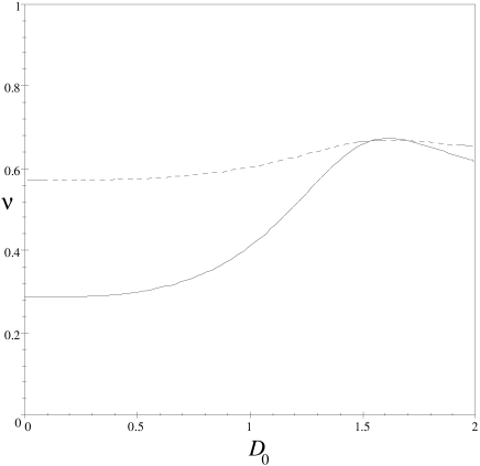
Figure 9.2: Test of the relation in Eq. (9.4) for the Ising-model in $d=2.25,\ d=2.5,\ d=2.75$ and $d=3$. The upper curves are from the high temperature representations of the Ising model ($D=1$), while the lower curves are from the low temperature expansion ($D=d-1$) as explained in the text. The exponent $\nu$ is extrapolated from the maximum of each curve. These curves are based on the scheme in which we extrapolate $\nu d$, linearize in $N$, and to divide the result by $dD$. This choice is determined through the quality checks of section 7.

We shall now test the validity of the above conjecture. As discussed before, our generalization to the sum over manifolds is defined only up to the factor $c(D)$. For the remainder of this section we make the “least number of variables” choice $c(D)=D$, for the partition function. Singularities of the partition function are characterized by the critical exponent $\alpha(D,d,N)$, through

$$\ln{\mathcal{Z}}_{\mbox{\scriptsize singular}}\sim|t-t_{c}|^{2-\alpha}\ .$$ (9.1)

The equality of the singularities on approaching the critical point from the low or high temperature sides, requires

$$\alpha(1,d,1)=\alpha(d-1,d,1)\ .$$ (9.2)

From the scaling-relation

$$\alpha(D,d,1)=2-\frac{\nu(D,d,1)d}{D}$$ (9.3)

we obtain

$${\nu(1,d,1)}=\frac{1}{d-1}\,\nu(d-1,d,1)\ .$$ (9.4)

A more general identity is obtained by considering a generalized class of Ising models, whose interactions are defined on $D$-dimensional primitive elements of a lattice  [?]. In the standard Ising model the interactions occur on bonds ($D=1$), while in Ising lattice gauge theory interactions are placed on plaquettes ($D=2$). Equating the singularities from the high and low temperature expansions of such models, and assuming a single continuous phase transition, yields

$${\nu(D,d,1)}=\frac{D}{d-D}\,\nu(d-D,d,1)\ .$$ (9.5)

The conjectured identity in Eq. (9.4) was tested numerically, and the results are presented in Fig. 9.2. The extrapolated exponents (the maxima of the curves) from the dual high and low temperature expansions are in excellent agreement. Indeed, one could hardly expect better from a 1-loop calculation. Nevertheless, higher-loop calculations would be useful to check this surprising hypothesis. One of the peculiarities of the 1-loop extrapolations presented in Fig. 9.2 is that any crossing of the curves from the dual models occurs at the mean–field value of $2D/d$ from Eq. (8.23). This is accidental, but present for all of our “good” extrapolation variables. An explicit counter example is given on Fig. 9.4, where we used the “bad” extrapolation-variables $1/D$ and $d$. They are bad, as there is no pronounced maximum to estimate $\nu$. Nevertheless, the intersection of the two dual models occurs at $\nu=0.6$, not too far from the exact result of 0.6315.

Figure 9.4: Extrapolations for the Ising model and its dual in $D=1$, $d=3$, using $c(D)=D$, and as extrapolation variables $1/D$ and $d$.

10 Cubic anisotropy

Up to now, we assumed that the interaction between manifolds is independent of their color. This is a consequence of the rotational invariance of the underlying spin model introduced in Sec. 2. This equality of interactions does not have to hold in a system of polymer loops. In the context of the $\varphi^{4}$-theory, unequal interactions result from the breaking of rotational symmetry, e.g. through the introduction of cubic anisotropy, as discussed in Refs.  [?,?,?,?]. In the microscopic spin model of Sec. 2, the independence of the interactions between loops from their colors emerges as a consequence of the normalization condition

$$\sum_{i}S_{i}^{2}=1\ .$$ (10.1)

If we replace this by the constraint

$$\sum_{i}|S_{i}|^{a}=1\ ,$$ (10.2)

with $a\neq 2$, which breaks rotational symmetry, this is no longer the case.

The model in the absence of full spherical symmetry is described by two interaction parameters. In addition to $b$ which indicates the interaction between any two membranes irrespective of their color, there is a new anisotropic coupling constant $u$ which acts only between membranes of the same color. Physically, not all combinations of $u$ and $b$ are allowed, as some of them induce a collapse of the membranes. The following two cases can be distinguished:

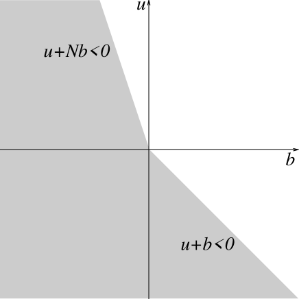
Figure 10.2: Regions of stability for the bare model with cubic anisotropy (the white portions are stable): The bare model is unstable if $u+Nb<0$ for $u>0$, and if $u+b<0$ for $u<0$. Note that this diagram changes upon renormalization.

(i) If $u$ is negative, for a single membrane to avoid itself and not to collapse, the condition

$$u+b>0\ ,$$ (10.3)

has to hold. This implies that $b$ is positive, and the repulsive interactions between any pair of membranes ensures mutual stability. The same condition is obtained in the $O(N)$-model by requiring the stability of the minimum energy state  [?].

(ii) If $u$ is positive, the stability condition in the $O(N)$-model is  [?]

$$u+Nb>0\ .$$ (10.4)

This places a lower bound on $b$ which is, for more than one color ($N>1$), more restrictive than Eq. (10.3), but still admits negative values for $b$ (see Fig. 10.2). For $b<0$, membranes of different color attract; in the extreme limit becoming glued together to form a “super-membrane” out of $N$ differently colored membranes. In this limit, the theory reduces to an Ising-like system, where the effective number of colors is one. (The corresponding RG-flows, as discussed below, do indeed tend to an Ising fixed point.) For this “super-membrane” not to collapse, we again find the condition in Eq. (10.4). However, this picture is quite schematic, and real physical systems are governed by many more parameters, and may well behave differently. Studies in polymers  [?,?] indicate that the precise competition of the attractive and repulsive parts of the interaction potential plays a crucial role, sometimes leading to non-universal behavior.

The above stability arguments are based on energetic considerations, and are expected to be modified upon the inclusion of fluctuations, say through a renormalization group procedure. In the studies of critical phenomena, a well-known example is the Coleman-Weinberg mechanism  [?,?], where the RG flows take an apparently stable combination of $b$ and $u$ into an unstable regime, indicating that fluctuations destabilize the system. In the flow diagrams described below, we also find the reverse behavior in which an apparently unstable combination of $b$ and $u$ flows to a stable fixed point. We interpret this behavior as indicating that fluctuations actually stabilize the model, a reverse Coleman-Weinberg effect, which to our knowledge has not been discussed before. To decide whether a system with a given combination of couplings is stable, we first follow the renormalization group flow. As perturbative renormalization does not say anything about the strong coupling regime, we regard run-away-trajectories in the flow as indicating an unphysical situation. If, on the other hand the renormalization group flow tends to a finite and completely IR-stable fixed point, we use the “classic” stability analysis discussed above, since renormalization has eliminated all fluctuations. Using this criterion we have shaded in grey the unphysical regions in the following flow diagrams.

The derivation of the generalized renormalization group functions is most easily carried out in a mixed scheme, in which we absorb contributions due to self-avoidance into $Z$, and those due to interactions with another membrane (proportional to $N$) into $Z_{t}$. For the original model, this scheme leads to the renormalization factors

$$Z_{t}(b) = 1+\frac{b}{2\varepsilon}\frac{Nc(D)}{2}\ ,$$

$$Z(b) = 1+\frac{2-D}{2D}\frac{b}{\varepsilon}\ .$$ (10.5)

The presence of the additional interaction $u$ between membranes of the same color, modifies the above result to

$$Z_{t}(b,u) = 1+\frac{bNc(D)}{4\varepsilon}+\frac{uc(D)}{4\varepsilon}\ ,$$

$$Z(b,u) = 1+\frac{2-D}{2D}\frac{b+u}{\varepsilon}\ .$$ (10.6)

To derive the renormalization of the coupling-constants, we note that with this choice of $Z$ and $Z_{t}$, we have eliminated all divergent configurations which in the polymer picture and in the MOPE are denoted by

$$\!\!\!\raisebox{-7.96661pt}{ \begin{picture}(25.0,12.0)(0.0,0.0)\put(10.0,5.0){\put(0.0,0.0){\circle*{2.0}} \put(-5.0,5.0){\circle*{2.0}} \put(-5.0,-5.0){\circle*{2.0}} \put(-10.0,0.0){\oval(20.0,10.0)[r]} \put(-5.0,-5.0){\dashbox(0.5)(0.0,10.0)[]{}} \put(0.0,0.0){\dashbox(0.5)(5.0,0.0)[]{}} \put(5.0,0.0){\put(0.0,0.0){\circle*{2.0}}} \put(15.0,0.0){\oval(20.0,10.0)[l]} }\end{picture}}\ ,\quad\mbox{ and}\qquad\,\parbox{43.53232pt}{\epsfbox{./gnondiv.eps}}\,\ ,$$ (10.7)

respectively. The diagrams that renormalize the interactions are of two classes

$${\!\!\!\raisebox{-12.94582pt}{ \begin{picture}(15.0,15.0)(0.0,0.0)\put(5.0,5.0){ \put(10.0,2.5){\oval(10.0,15.0)[l]} \put(-5.0,2.5){\oval(10.0,15.0)[r]} \put(0.0,0.0){\circle*{2.0}} \put(0.0,5.0){\circle*{2.0}} \put(0.0,0.0){\circle*{2.0}} \put(0.0,0.0){\dashbox(0.5)(5.0,0.0)[]{}} \put(0.0,5.0){\dashbox(0.5)(5.0,0.0)[]{}} \put(5.0,0.0){\circle*{2.0}} \put(5.0,5.0){\circle*{2.0}} }\end{picture}}}\ ,\qquad\mbox{\rm and}\qquad\!\!\!\raisebox{-7.96661pt}{ \begin{picture}(30.0,10.0)(0.0,0.0)\put(10.0,5.0){ \put(-5.0,0.0){\dashbox(0.5)(5.0,0.0)[]{}} \put(-5.0,0.0){\circle*{2.0}} \put(0.0,0.0){\circle*{2.0}} \put(-10.0,0.0){\oval(10.0,10.0)[r]} \put(5.0,0.0){\circle{10.0}} \put(10.0,0.0){\dashbox(0.5)(5.0,0.0)[]{}} \put(20.0,0.0){\oval(10.0,10.0)[l]} \put(10.0,0.0){\circle*{2.0}} \put(15.0,0.0){\circle*{2.0}} }\end{picture}}\ .$$ (10.8)

In calculating the contribution to the renormalization of $b$, the inner loop of the latter diagram contributes a factor of $N$ if both interactions are $b$, and 1 for the two cases when one of the interactions is $u$, resulting in

$$b = \mu^{-\varepsilon}Z^{-\frac{d}{2}}\left(1-\frac{b}{\varepsilon}\mbox{Res}\bigg{<}\!\,\parbox{38.41095pt}{\epsfbox{./gm_quer.eps}}\,\bigg{|}\,\parbox{30.72867pt}{\epsfbox{./gb.eps}}\,\!\bigg{>}-b\frac{Nc(D)}{4\varepsilon}-u\frac{c(D)}{2\varepsilon}\right)b_{0}\ .\quad$$ (10.9)

(Note that because of the choice of the mixed RG scheme, the above relation does not reduce for $u=0$ to the corresponding one derived earlier.) For the anisotropic coupling $u$, the first class of diagrams can be constructed from two interactions $u$ (1 way), or one $u$ and one $b$ (two ways). The second class gives a single contribution proportional to $u^{2}$, for the overall result

$$u = \mu^{-\varepsilon}Z^{-\frac{d}{2}}\times\left(1-\frac{u+2b}{\varepsilon}\mbox{Res}\bigg{<}\,\parbox{38.41095pt}{\epsfbox{./gm_quer.eps}}\,\bigg{|}\,\parbox{30.72867pt}{\epsfbox{./gb.eps}}\,\bigg{>}-u\frac{c(D)}{4\varepsilon}\right)u_{0}\ .$$ (10.10)

The renormalized parameters yield the $\beta$-functions at 1-loop order, as

$$\beta_{b}(b,u) = -\varepsilon b+b^{2}\left(\mbox{Res}\bigg{<}\,\parbox{38.41095pt}{\epsfbox{./gm_quer.eps}}\,\bigg{|}\,\parbox{30.72867pt}{\epsfbox{./gb.eps}}\,\bigg{>}+1+\frac{Nc(D)}{4}\right)+\,bu\left(1+\frac{c(D)}{2}\right)\ ,$$

and

$$\beta_{u}(b,u) = -\varepsilon u+u^{2}\left(\mbox{Res}\bigg{<}\,\parbox{38.41095pt}{\epsfbox{./gm_quer.eps}}\,\bigg{|}\,\parbox{30.72867pt}{\epsfbox{./gb.eps}}\,\bigg{>}+1+\frac{c(D)}{4}\right)$$ (10.12)

$$+\,bu\left(1+2\mbox{Res}\bigg{<}\,\parbox{38.41095pt}{\epsfbox{./gm_quer.eps}}\,\bigg{|}\,\parbox{30.72867pt}{\epsfbox{./gb.eps}}\,\bigg{>}\right)\ .$$

Finally, the exponent $\nu$ is obtained from Eq. (10) as

$$\nu(b,u)=\frac{2-D}{2}\left(1+\frac{1}{2D}\left[b\left(1+\frac{Nc(D)}{2}\right)+u\left(1+\frac{c(D)}{2}\right)\right]\right)\ .$$ (10.13)

For $D\to 1$, these equations reduce to the renormalization-group functions reproduced in Amit  [?]. (In  [?] there is an additional factor of 2/3 due to the choice of numerical constants.)

As in their standard counterpart, these flow-equations admit 4 fixed points:

1. The Gaussian fixed point

   $$b^{*}_{G}=0\ ,\quad u^{*}_{G}=0\ ,$$ (10.14)

   which is always unstable below the upper critical line $d_{u}(D)$. (The following discussions of stability all pertain to this region.)

2. The Heisenberg fixed point

   $$b^{*}_{H}=\frac{\varepsilon}{1+\frac{Nc(D)}{4}+\mbox{Res}\bigg{<}\,\parbox{38.41095pt}{\epsfbox{./gm_quer.eps}}\,\bigg{|}\,\parbox{30.72867pt}{\epsfbox{./gb.eps}}\,\bigg{>}}\ ,\quad u^{*}_{H}=0\ ,$$ (10.15)

   is always stable along the $u=0$ axis, and is completely stable as long as

   $$\frac{Nc(D)}{4}<\mbox{Res}\bigg{<}\,\parbox{38.41095pt}{\epsfbox{./gm_quer.eps}}\,\bigg{|}\,\parbox{30.72867pt}{\epsfbox{./gb.eps}}\,\bigg{>}_{\varepsilon^{-1}}\ .$$ (10.16)

   This certainly applies to single polymers and membranes with $N=0$, but is also the case for the $O(N)$ model as long as $N<4$.

3. The Ising fixed point

   $$b^{*}_{I}=0\ ,\quad u^{*}_{I}=\frac{\varepsilon}{1+\frac{c(D)}{4}+\mbox{Res}\bigg{<}\,\parbox{38.41095pt}{\epsfbox{./gm_quer.eps}}\,\bigg{|}\,\parbox{30.72867pt}{\epsfbox{./gb.eps}}\,\bigg{>}}\ ,$$ (10.17)

   is stable if

   $$\mbox{Res}\bigg{<}\,\parbox{38.41095pt}{\epsfbox{./gm_quer.eps}}\,\bigg{|}\,\parbox{30.72867pt}{\epsfbox{./gb.eps}}\,\bigg{>}<\frac{c(D)}{4}\ .$$ (10.18)

   For the standard $O(N)$-model with $D=1$ the Ising fixed point is unstable. However, since for large $d_{c}$, the left hand side of the above inequality decays rapidly as $2^{-d_{c}/2}$, the Ising fixed point is stable if the expansion point is sufficiently close to $D=2$.

4. The cubic fixed point is located at

   $$b^{*}_{c} = \frac{\left(A(D)-\frac{c(D)}{4}\right)}{\left(1+\frac{Nc(D)}{4}+A(D)\right)\left(A(D)-\frac{c(D)}{4}\right)+\left(1+\frac{c(D)}{2}\right)\left(\frac{Nc(D)}{4}-A(D)\right)}\varepsilon\ ,$$

   $$u^{*}_{c} = \frac{\left(\frac{Nc(D)}{4}-A(D)\right)}{\left(1+\frac{Nc(D)}{4}+A(D)\right)\left(A(D)-\frac{c(D)}{4}\right)+\left(1+\frac{c(D)}{2}\right)\left(\frac{Nc(D)}{4}-A(D)\right)}\varepsilon\ ,$$ (10.19)

   $$\mbox{where}\qquad A(D)=\mbox{Res}\bigg{<}\,\parbox{38.41095pt}{\epsfbox{./gm_quer.eps}}\,\bigg{|}\,\parbox{30.72867pt}{\epsfbox{./gb.eps}}\,\bigg{>}\ .$$

   The stability of this point under RG flows depends on the parameters $D$ and $N$, and this dependence is not simple. The physical stability of this fixed point according to the criteria of Eqs. (10.3) and (10.4) should also be verified. Interestingly, we find (at least at 1-loop order) that whenever the fixed point is IR-stable, it falls in the physically stable region. Note that there are combinations of $D$ and $N$, for which the cubic fixed point is at infinity in the 1-loop approximation. An explicit example is for $D=1$ and $N=0$, a scenario relevant to the random bond Ising model discussed in the next section.

Figure 10.4: Regions with different RG flow patterns in the $(N,D)$-plane, as discussed in the text. The domain-boundaries are obtained from $c(D)=4A(D)$ for the line separating (iii) and (iv) as well as (ii) and (vi); $Nc(D)=4A(D)$ for the line separating (i) and (ii) as well as (iv) and (v). A third boundary is given by the vanishing of the denominator in Eq. (10.19).

The two RG equations admit six different flow patterns, the last four of which do not occur in the standard field theory. The domains of the $(N,D)$ plane corresponding to each of the following scenarios is plotted in Fig. 10.4:

1. For $D=1$, i.e. in the case of the $O(N)$ model, and for $0<N<4$, only the Heisenberg fixed point is stable, as indicated in Fig. 10.6. This is the fixed point that is usually studied in the context of critical phenomena.

2. For $D=1$ and $N>4$, the Heisenberg fixed point is unstable and the system is governed by the cubic fixed point (Fig. 10.8).

3. An interesting phase diagram is obtained for $N=0$ and $1<D<1.29$. Then, as shown in Fig. 10.10, the Heisenberg and cubic fixed points are both stable, their domains of attraction being separated by the axis $b=0$.

4. Another phase diagram with two completely stable fixed points is obtained for $N=0$ and $D$ close to 2. Then, as shown in Fig. 10.12, the Heisenberg and Ising fixed points are both stable, and there is a phase separatrix passing through the Gaussian and the cubic fixed points.

5. For $D$ close to 2 and $N>N_{c}$, where $N_{c}$ vanishes exponentially for $D\to 2$, the cubic fixed point is in the lower right sector. Both the cubic and Ising fixed points are stable as indicated in Fig. 10.14.

6. Yet another possibility is that both the Heisenberg and the cubic fixed points are unstable, as in Fig. 10.16. This is the case for $D$ close to 2 and $N$ large. Then only the Ising fixed point is attractive and controls the critical behavior.

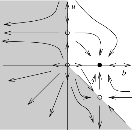
Figure 10.6: RG-flow from Eqs. (10) and (10.12) in domain (i), e.g. $D=1$ and $N<4$; shaded regions are unstable.

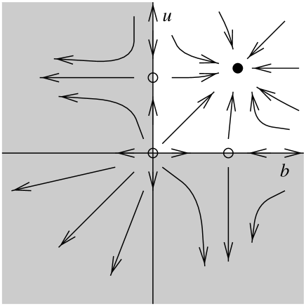
Figure 10.8: RG-flow from Eqs. (10) and (10.12) in domain (ii), e.g. $D=1$ and $N>4$; shaded regions are unstable.

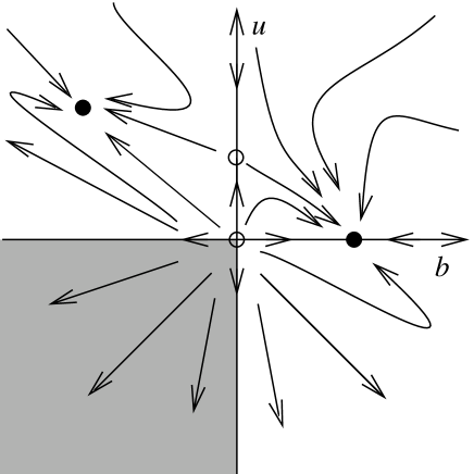
Figure 10.10: RG-flow from Eqs. (10) and (10.12) in domain (iii), e.g.  $N=0$ and $1<D<1.29$, shaded regions being unstable.

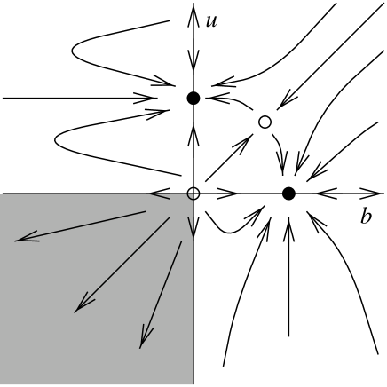
Figure 10.12: RG flow from Eqs. (10) and (10.12) in domain (iv), e.g.  $N=0$ and $D$ close to 2; shaded regions are unstable.

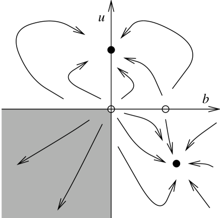
Figure 10.14: RG-flow from Eqs. (10) and (10.12) in domain (v), e.g.  $N=0.2$ and $D=1.8$, shaded regions being unstable.

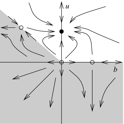
Figure 10.16: RG flow from Eqs. (10) and (10.12) in domain (vi), e.g.  large $N$ and $D$ close to 2; shaded regions are unstable.

We may inquire as to how the above flow diagrams, with different stable points and stability regions, can occur by continuously moving around in the $(N,D)$ plane. To demonstrate this, let us examine the sequence of flow diagrams for $N=0$ and differing $D$. The appropriate flow diagram for $D<1$ is that of Fig. 10.6, with the cubic fixed point going to infinity as $D\to 1$. For $D>1$ this fixed point reappears in the upper left sector, as in Fig. 10.10. Along the way, it coincides with the stable fixed point at infinity, and they exchange stability. This mechanism of changing stability from one fixed point to another is quite general, and occurs again when the cubic and Ising fixed points merge at $D\approx 1.29$. For $1.29<D<2$, the appropriate flow diagram is that of Fig. 10.12. The cubic fixed point continues to approach the Heisenberg one as $D\to 2$, resulting in very slow approaches to the fixed points in this limit.

We may ask whether the expanded picture presented here provides any new insight into the behavior of tethered self-avoiding membranes ($D=2$, $N=0$). The perturbative expansion predicts a crumpled phase with an exponent of $\nu=0.85<1$ in $d=3$  [?,?]. Yet many simulations of this system using models of beads and springs  [?,?,?,?,?] seem to suggest a flat phase with $\nu=1$. It is thus important to ask if there are additions to the standard description of such membranes in Eq. (5.3), which can lead to a flat configuration. The most natural candidate is a bending rigidity $\kappa$, which is automatically generated in models of strings and beads as pointed out in Ref.  [?]. However, it is expected that a finite $\kappa_{c}$ is needed in a flat phase, while the absence of a crumpled phase in simulations may suggest $\kappa_{c}=0$. Our modified Hamiltonian with cubic anisotropy indicates that the presence of even small $u$ for $D\to 2$ places the system within the domain of attraction of the Ising fixed point in Fig. 10.12. (The separatrix through the cubic fixed point approaches the horizontal line as $D\to 2$.) The exponents that we calculate for the Ising fixed point ($\nu>1$ in $d=3,4$ and $\nu=0.9$ in $d=5$, $\nu=0.8$ in $d=6$, and $\nu=0.6$ in $d=8$) are tantalizingly close to those found in the simulations of Grest  [?]. Yet it is hard to justify the inclusion of a finite $u$, which is meaningless for a single membrane at $N=0$. While the presence of additional membranes does limit the bending of the membranes around it, the net effect is much more than just a simple bending rigidity, as related constraints appear on all length scales.

11 The random bond Ising model

In this section we analyze in greater detail the model for $N=0$. The $N\to 0$ limit is interesting, not only because of its relevance to self-avoiding polymers and membranes, but also for its relation to the Ising model with bond disorder. To show the latter connection, we start with the field theory description of the random bond Ising model, with the Hamiltonian

$${\mathcal{H}}=\int_{r}\left[\frac{1}{2}\left(\nabla S(r)\right)^{2}+\frac{1}{2}\left(t+\eta(r)\right)S^{2}(r)+uS^{4}(r)\right]\ ,$$ (11.1)

where $\eta(r)$ is a quenched random variable (with $\overline{\eta(r)}=0$). Expectation values with quenched disorder can be calculated from a partition function that is replicated $N$ times, in the limit $N\to 0$ (for a review see e.g.  [?]). Averaging the replicated weight over the Gaussian random variable $\eta(r)$, with $\overline{\eta(r)\eta(r^{\prime})}=2\sigma\delta^{d}(r-r^{\prime})$, induces an interaction between different replicas with an effective Hamiltonian

$${\mathcal{H}}_{N}=\int_{r}\sum_{\alpha}\left[\frac{1}{2}\left(\nabla S_{\alpha}(r)\right)^{2}+\frac{t}{2}S_{\alpha}^{2}(r)+uS_{\alpha}^{4}(r)\right]-\sigma\sum_{\alpha\beta}S_{\alpha}^{2}(r)S_{\beta}^{2}(r)\ .$$ (11.2)

The replicated system is thus controlled by a Hamiltonian with positive cubic anisotropy $u$, but negative $b=-\sigma$.

A key result in the study of random bond systems is the ”Harris criterion” [?], which states that randomness is relevant as long as the heat capacity exponent $\alpha$ is positive. This is the case for the Ising model, and therefore new critical behavior is expected for the random bond system. In the usual field theory treatments  [?,?,?,?], there is no fixed point at the 1-loop order. This is due to the vanishing of the denominator in Eq. (10.19) for $D=1$. However, we now have the option of searching for a stable fixed point by expanding about $D\neq 1$. Indeed, for $N=0$ and $1<D<1.29$, the cubic fixed point lies in the upper left sector ($u>0$ and $b<0$) and is completely stable, see Figs. 10.10 and 11.2. The extrapolation for $\nu$ at the cubic fixed point is plotted in Fig. 11.4, where it is compared to the results for the Heisenberg and Ising fixed points. The divergence of $\nu$, upon approaching $D=1$ from above, is a result of the cubic fixed point going to infinity as mentioned earlier. Upon increasing $D$, the Ising and cubic fixed points approach each other, and merge for $D=1.29$. For larger values of $D$, the cubic fixed point is to the right of the Ising fixed point ($b_{c}^{*}>0$) and only the latter is stable. Given this structure, no plateau can be found for a numerical estimate of the random bond exponent $\nu_{\mbox{\scriptsize DO}}$, and we can only posit the inequality

$$\nu_{\mbox{\scriptsize DO}}>\nu_{\mbox{\scriptsize Ising}}\ .$$ (11.3)

While Eq. (11.3) was derived at 1-loop order, it should hold at higher orders, if no drastic subleading corrections appear; since it merely depends on the general structure of the renormalization group flow.

Higher loop calculations of the random bond Ising model can be used to expand the exponent $\nu$ in powers of $\sqrt{\varepsilon}$. Eq. (11.3) can then be compared to the 2-loop result  [?], which in $d=3$ reads

$$\nu_{\mbox{\scriptsize DO}}=\frac{1}{2}+\sqrt{\frac{6}{53}}\frac{1}{4}\approx 0.584\ .$$ (11.4)

This is slightly larger than the corresponding Ising value at 1-loop order ($\nu\approx 0.583$), but smaller than the best known Ising result ($\nu\approx 0.631$). Three- and four-loop calculations were performed in Refs.  [?] and  [?] respectively; the latter gives $\nu=0.6714$ and $\nu=0.6680$ depending on the resummation-method used. Two-loop calculations in fixed dimension $d=3$  [?] yield $\nu=0.678$. A similar result is obtained within a modified Padé-Borel approximation of 3-loop results in Ref. [?], yielding $\nu=0.666$. We also note that Ref. [?] stresses the existence of very slow transients in the renormalization group flow for small $\varepsilon$. The extremely retarded crossover to the random bond fixed point may quantitatively explain the Monte-Carlo data which seem to suggest a disorder-dependent, and thus non-universal, behavior for the critical exponents. The same characteristic flow is also present at 1-loop order for our random bond fixed point candidate, e.g. for $D=1.1$ as in Fig. 11.2, further validating our approach.

Figure 11.2: Renormalization group flows for $D=1.1$ and $N=0$. The cubic fixed point is marked by a diamond

Within error-bars, all these results are consistent with $\alpha=0$, i.e. the border-line value of the Harris criterion [?], corresponding to

$$\nu=\frac{2}{3}\ .$$ (11.5)

There is also an exact result [?] that the exponent $\nu$ in any random system must be greater than or equal to $2/d$. Generalizing the “Harris criterion” bound to manifolds yields a limiting value of $2D/d$, which is also the mean–field value discussed earlier.

Figure 11.4: Extrapolations of $\nu$ from the expansion of $\nu d$ with $c(D)=D$, for the $O(N)$-model in three dimensions. The values of the Heisenberg fixed point for $N=0$ are compared to those of the Ising and cubic fixed points. The crossing of the latter two curves yields an estimate of $\nu=0.6315$ for the $d=3$ Ising model.

The duality between the high and low temperature expansions of the Ising model remains valid in the presence of random bonds. As discussed above, the high temperature expansion can be presented geometrically as a theory of loops with self-avoidance ($u>0$), and mutual attraction ($b<0$). We can develop a related low temperature expansion as follows: Starting with an ordered ground state, the partition function $Z[\{J\}]$ can be expanded as a sum over contributions of droplets of the opposite spin; each element of the droplet surface crossing a local random bond $J$ makes a contribution of $\exp(-2\beta J)$. A replicated description is obtained for $Z[\{J\}]^{N}$ as a sum over droplets of $N$ different colors. The next step is to average over all the random bonds $\{J\}$: A specific bond may be crossed $m=0,1,\ldots,N$ times for a given term in $Z[\{J\}]^{N}$. Assuming that the random bonds are independently chosen from a Gaussian distribution of width $\sigma$, each random bond contributes a factor of

$$\overline{\exp(-2\beta mJ)}=\exp\left[-2\beta\left(\overline{J}-\beta\sigma\right)m+4\beta^{2}\sigma\,\frac{m(m-1)}{2}\right].$$ (11.6)

The first term in the exponent on the right hand side can be regarded as a shift in the bond energy due to randomness. The second term represents a pairwise attraction between the $m$ manifolds of different colors. Thus the quench averaged low temperature description is of a set of $D=d-1$ dimensional self-avoiding droplets, with mutual attractions between droplets of different colors. (This is easily generalized to models with interactions defined on other elementary manifolds.)

We can now make the conjecture that the low temperature sums are not drastically modified by restricting the droplets to tethered membranes. This will again lead to the exponent identity in Eq. (9.5). The extrapolations from the dual descriptions of the random bond Ising model (at the cubic fixed point) are presented in Fig. 11.6. Because of the absence of a plateau, there are no clear points where these curves can be compared. The intersection of the two curves provides a specific point for extracting exponents of the random bond model. However, as discussed in section 9, at the 1-loop level this occurs at the mean-field value of $2/3$.

Figure 11.6: Extrapolations of $\nu$ from the expansion of $\nu d$ with $c(D)=D$, for the random bond Ising-model in $d=3$, from the high and low temperature descriptions. Note that the intersection of the curves (from these dual descriptions) at the mean-field value of 2/3 is a property of the 1-loop expansion, as discussed in section 9.

In the previous sections we relied on a plateau in the extrapolation curves to obtain numerical values of the exponents. Another method for selecting a specific point of these curves is to look at intersection points. For example, in Fig. 11.4 the curves corresponding to the cubic and Ising fixed points intersect at $D=1.29$. Since the intersection occurs when the two fixed points coalesce on the $b=0$ axis, they both have Ising symmetry at this junction. We may hope that this point yields precise exponents as all ambiguity in the expansion point is removed. The actual numerical prediction of

$$\nu^{*}=0.6315\ ,$$ (11.7)

is indistinguishable from higher-order calculations  [?]. However, the method is not insensitive to the extrapolation variables used, and it is thus unclear if more precise results are obtained in higher order calculations.

Finally, we note that the above considerations are easily generalized to multi-component spins subject to random bonds. We shall denote the number of components of the field by $p$, reserving the symbol $N$ for the number of replicas, as in the random bond Ising model (corresponding to $p=1$). Starting as in Eq. (11.1) from

$${\mathcal{H}}^{p}=\int_{r}\sum_{i=1}^{p}\left[\frac{1}{2}\left(\nabla S^{i}(r)\right)^{2}+\frac{1}{2}\left(t+\eta(r)\right)S^{i}(r)^{2}\right]+u\sum_{i,j=1}^{p}S^{i}(r)^{2}S^{j}(r)^{2}\ ,$$ (11.8)

yields in analogy with Eq. (11.2), after replicating and averaging over $\eta$,

$${\mathcal{H}}^{p}_{N}=\!\int_{r}\sum_{\alpha=1}^{N}\sum_{i=1}^{p}\left[\frac{1}{2}\!\left(\nabla S^{i}_{\alpha}(r)\right)^{2}\!\!+\!\frac{t}{2}S^{i}_{\alpha}(r)^{2}\right]+u\!\sum_{\alpha=1}^{N}\sum_{i,j=1}^{p}S_{\alpha}^{i}(r)^{2}S_{\alpha}^{j}(r)^{2}-\sigma\!\!\sum_{\alpha,\beta=1}^{N}\sum_{i,j=1}^{p}S_{\alpha}^{i}(r)^{2}S^{j}_{\beta}(r)^{2}\ .$$ (11.9)

In the resulting $O(N)\times O(p)$-model, rotational symmetry is broken in the $O(N)$-sector, but remains intact in the $O(p)$-sector. We can next develop a geometrical description of the high temperature expansion of this field theory in the language of self-avoiding polymer loops, which are then generalized to membranes. It is then easy to see that in a perturbative expansion, each closed loop contributes an additional factor of $p$ (as in the standard $O(N)$-model, where every closed loop is accompanied by a factor of $N$). All previous results are thus simply generalized by replacing $c(D)$ in the renormalization group expressions with $p\times c(D)$. Since, according to the Harris criteorion [?], non-trivial random bond exponents are obtained in the physical dimensions of $d=2$ and $d=3$, only for $p\leq 2$, we shall not pursue this analogy further.

Appendix A Derivation of the RG-equations

In this section, we give a derivation of the renormalization group functions. Starting from

$$b=b_{0}\,Z_{b}^{-1}\,Z^{-d/2}\,\mu^{-\varepsilon}\ ,$$ (A.1)

the $\beta$-function is given through the variation of the renormalized coupling, at fixed values of the bare coupling and bare chemical potential, as

$$\beta(b):=\mu\frac{\partial}{\partial\mu}\parbox{2.84526pt}{ \begin{picture}(1.0,12.0)\put(0.5,-0.2){\line(0,1){11.0}} \end{picture} }_{0}b\ .$$ (A.2)

From the derivative of Eq. (A.1) with respect to $\mu$, we obtain

$$\beta(b)\left(1+b\frac{\partial}{\partial b}\ln(Z_{b}Z^{d/2})\right)=-\varepsilon b\ ,$$ (A.3)

which solving for $\beta(b)$, yields

$$\beta(b)=\frac{-\varepsilon b}{1+b\frac{\partial}{\partial b}\ln(Z_{b}Z^{d/2})}\ .$$ (A.4)

The scaling exponent $\nu$ relates the chemical potential $t$ and radius of gyration $R$ through

$$R\sim t^{-\nu/D}\ .$$ (A.5)

To obtain $\nu$, we first observe that the dimensionless combination $R^{2}t^{\frac{2-D}{D}}$, is a function of $b$ and $t/\mu^{D}$ only, i.e.

$$R^{2}t^{\frac{2-D}{D}}=f(b,t/\mu^{D})\ .$$ (A.6)

Since in addition, $t$ can be expressed as a function of $t_{0}$ and $b$ only, Eq. (A.6) implies that

$$\mu\frac{\mbox{d}}{\mbox{d}\mu}\left[R^{2}t^{\frac{2-D}{D}}\right]=\left(\beta(b)\frac{\partial}{\partial b}-Dt\frac{\partial}{\partial t}\right)\left[R^{2}t^{\frac{2-D}{D}}\right]\ .$$ (A.7)

Next observe that $R_{0}^{2}t_{0}^{\frac{2-D}{D}}$ is independent of the renormalization scale $\mu$. Replacing bare by renormalized quantities, we obtain a relation for the total derivative with respect to $\mu$, as

$$\mu\frac{\mbox{d}}{\mbox{d}\mu}\left[R^{2}t^{\frac{2-D}{D}}Z(b)Z_{t}(b)^{\frac{2-D}{D}}\right]=0\ .$$ (A.8)

Combining the latter relation with Eq. (A.7) gives

$$\left(Dt\frac{\partial}{\partial t}-\beta(b)\frac{\partial}{\partial b}-\beta(b)\frac{\partial}{\partial b}\ln\left(ZZ_{t}^{\frac{2-D}{D}}\right)\right)\left[R^{2}t^{\frac{2-D}{D}}\right]=0\ .$$ (A.9)

The scaling function of the field, describing the scaling of the membrane at the critical point with $\beta(b)\to 0$, is thus

$$\nu(b)=\frac{2-D}{2}-\frac{1}{2}\beta(b)\frac{\partial}{\partial b}\ln\left(ZZ_{t}^{\frac{2-D}{D}}\right)\ .$$ (A.10)

(Note that the last term cannot be dropped, as the vanishing of the $\beta$-function is canceled by the divergence of the derivatives of the $Z$-factors at this point.)

Appendix B Reparametrization invariance

In this appendix, we shall explore the consequences of a reparametrization

$$x\longrightarrow x^{\prime}=x\,Z_{\alpha}^{-1/D}\ ,$$ (B.1)

on the Hamiltonian

$${\mathcal{H}} = \frac{Z}{2-D}\int_{x}\frac{1}{2}(\nabla r(x))^{2}+b\mu^{\varepsilon}Z_{b}\int_{x}\int_{y}\tilde{\delta}^{d}(r(x)-r(y))+tZ_{t}\Omega\ ,$$ (B.2)

for a self-avoiding membrane ($D=1$ for polymers). (The notation for the rescaling factor anticipates renormalization factors that we shall introduce next.) The Hamiltonian in Eq. (B.2) is in fact not invariant under this rescaling because of the cutoff implicit in the interaction. In order to achieve scale invariance, the cutoff, or equivalently the renormalization scale $\mu$, must also be rescaled to

$$\mu\longrightarrow\mu^{\prime}=\mu\,Z_{\alpha}^{1/D}\ .$$ (B.3)

The Hamiltonian then changes to

$${\mathcal{H}} = \frac{ZZ_{\alpha}^{\frac{2-D}{D}}}{2-D}\int_{x}\frac{1}{2}(\nabla r(x))^{2}+b\mu^{\varepsilon}Z_{b}Z_{\alpha}^{\varepsilon/D-2}\int_{x}\int_{y}\tilde{\delta}^{d}(r(x)-r(y))+tZ_{t}Z_{\alpha}^{-1}\Omega\ .\qquad$$ (B.4)

Comparing to the original Hamiltonian then identifies the new renormalization group factors

$$Z^{\prime} = ZZ_{\alpha}^{\frac{2-D}{D}}$$

$$Z_{t}^{\prime} = Z_{t}Z_{\alpha}^{-1}$$ (B.5)

$$Z_{b}^{\prime} = Z_{b}Z_{t}^{-2+\varepsilon/D}\ .$$

As discussed in the main text, see Eqs. (3.29) and (5.25), the renormalization group-functions are left unchanged by the transformations in Eqs. (B.5); the most useful case being $Z_{\alpha}=Z_{t}$.

Appendix C Structure of the divergences and the MOPE

In this appendix we present a more intuitive description of the structure of the divergences, and the multilocal operator product expansion (MOPE) used to prove renormalizability [?,?] and for explicit calculations  [?,?]. This presentation already appears in French in Ref.  [?], but is reproduced here for completeness, and convenience of readers.

We first remark that with our choice of normalizations, the free propagator

$$\frac{1}{d}\left<\frac{1}{2}\left(r(x_{1})-r(x_{2})\right)^{2}\right>_{0}=|x_{1}-x_{2}|^{2-D}\ ,$$ (C.1)

is the Coulomb potential in $D$ dimensions. This analogy with electrostatics will help us to analyze the structure of the divergences. The interaction part of the Hamiltonian $\mathcal{H}$ is reminiscent of a dipole, and can be written as

$${\mathcal{H}}_{\mbox{\scriptsize int}} = b\int_{x_{1}}\int_{x_{2}}\tilde{\delta}^{d}(r(x_{1})-r(x_{2}))$$ (C.2)

$$= b\int_{x_{1}}\int_{x_{2}}\int_{k}\mbox{e}^{ik(r(x_{1})-r(x_{2}))}\ .$$

The next step is to analyze the divergences appearing in the perturbative calculation of expectation values of observables. To simplify the calculations, we focus on the partition function

$${\mathcal{Z}}=\sum_{\mbox{\scriptsize all states}}\mbox{e}^{-\mathcal{H}}=\left<\mbox{e}^{-{\mathcal{H}}_{\mbox{\scriptsize int}}}\right>_{0}\ .$$ (C.3)

To exhibit the similarity to Coulomb systems, consider the second order term

$$\frac{1}{2}\left<{\mathcal{H}}_{\mbox{\scriptsize int}}^{2}\right> = \frac{b^{2}}{2}\int_{x_{1}}\int_{x_{2}}\int_{y_{1}}\int_{y_{2}}\int_{k}\int_{p}\left<\mbox{e}^{ik(r(x_{1})-r(x_{2}))}\mbox{e}^{ip(r(y_{1})-r(y_{2}))}\right>_{0}$$ (C.4)

$$= \frac{b^{2}}{2}\int_{x_{1}}\int_{x_{2}}\int_{y_{1}}\int_{y_{2}}\int_{k}\int_{p}\,\mbox{e}^{-E_{\mbox{\scriptsize c}}},$$

where $E_{c}$ is the Coulomb-energy of a configuration of dipoles with charges $\pm k$, and $\pm p$, respectively. More generally, for any Gaussian measure we have

$$\left<\mbox{e}^{i\sum_{i}k_{i}r(x_{i})}\right>_{0}=\mbox{e}^{-\frac{1}{2}\sum_{i,j}k_{i}k_{j}\left<(r(x_{i})-r(x_{j}))^{2}\right>_{0}}\ .$$ (C.5)

Since for any configuration of dipoles, specified by their coordinates and charges, the total charge is zero, the Coulomb-energy is bounded from below, i.e.

$$E_{\mbox{\scriptsize c}}\geq 0\ .$$ (C.6)

This implies that

$$\mbox{e}^{-E_{\mbox{\scriptsize c}}}\leq 1\ ,$$ (C.7)

and that the configurations which contribute most are those with minimal charge.

Let us apply the above observation to evaluating the integrals in Eq. (C.4). The basic idea is to look for classes of configurations which are similar. The integral over the parameter which indexes such configurations is the product of a divergent factor, and a “representative” operator. For the case of two dipoles, one with charge $k$ and the other with charge $p-k$ contracted together, one only sees a simple dipole with charge $p$ from far away, i.e.

$${\scriptstyle k\atop\scriptstyle p-k}{\,\parbox{42.67912pt}{\epsfbox{./gm_quer.eps}}\,}{\scriptstyle-k\atop\scriptstyle-p+k}\, \approx \,{\scriptstyle p}{\,\parbox{28.45274pt}{\epsfbox{./gb.eps}}\,}{\scriptstyle p}\ \times\ \mbox{e}^{-k^{2}(|s|^{2-D}+|t|^{2-D})}\ .$$

The second factor on the r.h.s. contains the dominant part of the Coulomb energy $E_{\mbox{\scriptsize c}}={k^{2}(|s|^{2-D}+|t|^{2-D})}$ of the interaction between the two dipoles; $s$ and $t$ are the distances between the contracted ends. The integral over $k$ is now factorized, and we obtain

$$\int_{k}\mbox{e}^{-k^{2}(|s|^{2-D}+|t|^{2-D})}=(|s|^{2-D}+|t|^{2-D})^{-d/2}\ .$$ (C.9)

We define the MOPE coefficient, as

$$\bigg{(}\,\parbox{38.41095pt}{\epsfbox{./gm_quer.eps}}\,\bigg{|}\,\parbox{30.72867pt}{\epsfbox{./gb.eps}}\,\bigg{)}=\left(|s|^{2-D}+|t|^{2-D}\right)^{-d/2}\ .$$ (C.10)

The MOPE therefore gives a convenient and powerful tool to calculate the dominant and all subdominant contributions from singular configurations.

For the sake of completeness, let us still calculate the two other MOPE coefficients used in the text. The first is for small $|x-y|$, ($\nu_{0}=\frac{2-D}{2}$)

$$\vphantom{\hbox{\,\parbox{20.48592pt}{\epsfbox{./gh.eps}}\,}}{}_{x}\,\parbox{20.48592pt}{\epsfbox{./gh.eps}}\,_{y} = \int_{k}\,:\mbox{e}^{ikr(x)}:\,:\mbox{e}^{-ikr(y)}:$$ (C.11)

$$= \int_{k}\,:\mbox{e}^{ik(r(x)-r(y))}:\mbox{e}^{-k^{2}|x-y|^{2\nu_{0}}}$$

$$= \int_{k}\left[\mbox{\bf 1}-\frac{k^{2}}{2d}\,:\left[r(x)-r(y)\right]^{2}:\,+\ldots\right]\mbox{e}^{-k^{2}|x-y|^{2\nu_{0}}}$$

$$= |x-y|^{-\nu_{0}d}\,\mbox{\bf 1}-\frac{1}{4}\,:\left[(x-y)\nabla r\left(\frac{x+y}{2}\right)\right]^{2}:\,|x-y|^{-\nu_{0}(d+2)}+\ldots$$

$$= |x-y|^{-\nu_{0}d}\,\mbox{\bf 1}\,-\frac{1}{2D}|x-y|^{D-\nu_{0}d}\,\,\parbox{10.24275pt}{\epsfbox{./go.eps}}\,\,+\ldots\ .$$

(The normal ordered operator $:\!\!O\!\!:$ indicates that all self-contractions of $O$ have been subtracted.) We also have to show the factorization property of    , which is the product of two $\tilde{\delta}^{d}$-interactions

$$\,\parbox{43.53232pt}{\epsfbox{./gnondiv.eps}}\,\raisebox{-14.08485pt}[0.0pt][0.0pt]{\makebox[0.0pt][l]{$\scriptstyle u\ \ \ x\,y\,z$} }=\int_{k,p}\,:\mbox{e}^{ikr(u)}:\,:\mbox{e}^{-ikr(x)}:\,:\mbox{e}^{ipr(y)}:\,:\mbox{e}^{-ipr(z)}:\ .$$ (C.12)

We want to study the contraction of $x$, $y$, and $z$, and look for all contributions which are proportional to

$$\,\parbox{30.72867pt}{\epsfbox{./gb.eps}}\,=\int_{k}\,:\mbox{e}^{ikr(u)}:\,:\mbox{e}^{-ikr((x+y+z)/3)}:\ .$$ (C.13)

The key-observation is that in Eq. (C.12) no contraction with $:\mbox{e}^{-ikr(x)}:$ contributes. All such contractions yield a factor of $k$, which after integration over $k$ results in derivatives of the $\tilde{\delta}^{d}$-distribution. This is equivalent to stating that as long as contributions proportional to     are studied, the following factorization property holds:

$$\,\parbox{43.53232pt}{\epsfbox{./gnondiv.eps}}\,=\,\parbox{30.72867pt}{\epsfbox{./gb.eps}}\,\times\,\parbox{20.48592pt}{\epsfbox{./gh.eps}}\,\ .$$ (C.14)

This is the reason why, in the massless scheme, divergences proportional to     are already eliminated through a counter-term for    , i.e. by the renormalization factor $Z$.

Appendix D Renormalization for infinite membranes

In this appendix, we give a short summary of the renormalization procedure for infinite membranes, and derive the one-loop counter-terms. This is a simplified version of the corresponding section in Ref.  [?], which is included here again mainly for completeness.

Let us start with a single dipole: When its end-points $(x,y)$ are contracted towards a point (taken here to be the center-of-mass $z=(x+y)/2$), the MOPE is

$$\vphantom{\hbox{\,\parbox{20.48592pt}{\epsfbox{./gh.eps}}\,}}_{x}\,\parbox{20.48592pt}{\epsfbox{./gh.eps}}\,_{y}=\bigg{(}\vphantom{\hbox{\,\parbox{20.48592pt}{\epsfbox{./gh.eps}}\,}}_{x}\,\parbox{20.48592pt}{\epsfbox{./gh.eps}}\,_{y}\bigg{|}\,\mbox{\bf 1}\bigg{)}\mbox{\bf 1}\ +\ \bigg{(}\vphantom{\hbox{\,\parbox{20.48592pt}{\epsfbox{./gh.eps}}\,}}_{x}\,\parbox{20.48592pt}{\epsfbox{./gh.eps}}\,_{y}\bigg{|}\,\parbox{10.24275pt}{\epsfbox{./go.eps}}\,\bigg{)}\,\parbox{10.24275pt}{\epsfbox{./go.eps}}\,\ +\ldots\ .$$

The first MOPE-coefficients are given explicitly by

$$\bigg{(}\vphantom{\hbox{\,\parbox{20.48592pt}{\epsfbox{./gh.eps}}\,}}_{x}\,\parbox{20.48592pt}{\epsfbox{./gh.eps}}\,_{y}\bigg{|}\,\mbox{\bf 1}\bigg{)} = |x-y|^{-\nu_{0}d}\ ,$$

$$\bigg{(}\vphantom{\hbox{\,\parbox{20.48592pt}{\epsfbox{./gh.eps}}\,}}_{x}\,\parbox{20.48592pt}{\epsfbox{./gh.eps}}\,_{y}\bigg{|}\,\parbox{10.24275pt}{\epsfbox{./go.eps}}\,\bigg{)} = -\frac{1}{2D}|x-y|^{D-\nu_{0}d}\ ,$$ (D.1)

and where     denotes the local operator

$$\,\parbox{10.24275pt}{\epsfbox{./go.eps}}\,=\frac{1}{2}(\nabla r(x))^{2}\ .$$ (D.2)

The integral over the relative distance $x-y$ for $\bigg{(}\vphantom{\hbox{\,\parbox{20.48592pt}{\epsfbox{./gh.eps}}\,}}_{x}\,\parbox{20.48592pt}{\epsfbox{./gh.eps}}\,_{y}\bigg{|}\,\parbox{10.24275pt}{\epsfbox{./go.eps}}\,\bigg{)}$ is, at $\varepsilon=0$, logarithmically divergent.

The simplest contraction resulting in a dipole is when two dipoles coalesce. The corresponding MOPE-coefficient is

$$\bigg{(}\,\parbox{38.41095pt}{\epsfbox{./gm_quer.eps}}\,\bigg{|}\,\parbox{30.72867pt}{\epsfbox{./gb.eps}}\,\bigg{)}=\left(|x|^{2\nu_{0}}+|y|^{2\nu_{0}}\right)^{-d/2}\ ,$$ (D.3)

where $x$ and $y$ are now the relative distances inside the two subsets. Another possibility is to consider the contraction    . But as we have shown in appendix C, this does not give a new divergence.

In the next step, counter-terms are introduced to subtract these divergences. We have to distinguish between counter-terms for relevant operators and those for marginal operators. The former can be defined by analytic continuation, while the latter require a subtraction scale. Indeed, the divergence for 1 is given by the integral

$$\int_{\Lambda^{-1}<|x-y|<L}\bigg{(}\vphantom{\hbox{\,\parbox{20.48592pt}{\epsfbox{./gh.eps}}\,}}_{x}\,\parbox{20.48592pt}{\epsfbox{./gh.eps}}\,_{y}\bigg{|}\mbox{\bf 1}\bigg{)} = \int_{\Lambda^{-1}}^{L}\frac{dx}{x}x^{D-\nu_{0}d}$$

$$= \frac{1}{D-\varepsilon}\left(\Lambda^{D-\varepsilon}-L^{\varepsilon-D}\right)\ ,$$

where $\Lambda$ is a high-momentum UV-regulator, and $L$ a large distance regulator. For $\varepsilon\approx 0$, this is UV-divergent but IR-convergent. The simplest way to subtract this divergence is therefore to replace the dipole operator by

$${}_{x}\,\parbox{30.72867pt}{\epsfbox{./gb.eps}}\,_{y}\ \longrightarrow\ _{x}\,\parbox{30.72867pt}{\epsfbox{./gb.eps}}\,_{y}\,-\,_{x}\,\parbox{30.72867pt}{\epsfbox{./gbdotted.eps}}\,_{y}\ ,$$ (D.5)

where ${}_{x}\,\parbox{30.72867pt}{\epsfbox{./gbdotted.eps}}\,_{y}=|x-y|^{-\nu_{0}d}$. This amounts to adding to the bare Hamiltonian, the UV-divergent counter-term

$$\Delta{\mathcal{H}}[r]=-{b\over 2}\,\int_{x}\int_{y}|x-y|^{-\nu_{0}d}\ ,$$ (D.6)

which is a pure number, and thus does not change the expectation value of any physical observable.

We next consider marginal operators: In the MOPE of Eq. (D), the integral over the relative distance of ${\displaystyle\int_{x-y}}\bigg{(}\vphantom{\hbox{\,\parbox{20.48592pt}{\epsfbox{./gh.eps}}\,}}_{x}\,\parbox{20.48592pt}{\epsfbox{./gh.eps}}\,_{y}\bigg{|}\,\parbox{10.24275pt}{\epsfbox{./go.eps}}\,\bigg{)}\,\parbox{10.24275pt}{\epsfbox{./go.eps}}\,$ is logarithmically divergent at $\varepsilon=0$. In order to find the appropriate counter-term, we use dimensional regularization, i.e. set $\varepsilon>0$. An IR-cutoff $L$, or equivalently a subtraction momentum scale $\mu=L^{-1}$, has to be introduced in order to define the subtraction operation. As a general rule, let us integrate over all distances appearing in the MOPE-coefficient, bounded by the subtraction scale $L=\mu^{-1}$, giving

$$\bigg{<}\,\parbox{20.48592pt}{\epsfbox{./gh.eps}}\,\bigg{|}\,\parbox{10.24275pt}{\epsfbox{./go.eps}}\,\bigg{>}_{L}:=\int_{|x-y|<L}\bigg{(}{}_{x}\,\parbox{20.48592pt}{\epsfbox{./gh.eps}}\,_{y}\bigg{|}\,\parbox{10.24275pt}{\epsfbox{./go.eps}}\,\bigg{)}=L^{\varepsilon}\,f(\varepsilon,D)\ .$$ (D.7)

Following Refs.  [?,?,?,?,?], we use a minimal subtraction scheme (MS). The internal dimension $D$ of the membrane is kept fixed, and Eq. (D.7) is expanded as a Laurent series in $\varepsilon$, which here starts at $\varepsilon^{-1}$. Denoting by $\mbox{Res}\big{<}\ \big{|}\ \big{>}$, the residue of the term of order $\varepsilon^{-1}$ of the Laurent expansion of $\big{<}\ \big{|}\ \big{>}_{L}$ for $L=1$, the residue of the pole in Eq. (D.7) is found to be

$$\mbox{Res}\bigg{<}\,\parbox{20.48592pt}{\epsfbox{./gh.eps}}\,\bigg{|}\,\parbox{10.24275pt}{\epsfbox{./go.eps}}\,\bigg{>}=-\frac{1}{2D}\ .$$ (D.8)

It is this pole that is subtracted in the MS-scheme by adding to the Hamiltonian a counter-term

$$\Delta{\mathcal{H}}[r]=-\frac{b}{\varepsilon}\,\mbox{Res}\bigg{<}\,\parbox{20.48592pt}{\epsfbox{./gh.eps}}\,\bigg{|}\,\parbox{10.24275pt}{\epsfbox{./go.eps}}\,\bigg{>}\,\int_{x}\,\parbox{10.24275pt}{\epsfbox{./go.eps}}\,_{x}\ .$$ (D.9)

Similarly, the divergence arising from the contraction of two dipoles into a single dipole is subtracted by a counter-term proportional to the residue of the single pole of

$$\bigg{<}\,\parbox{38.41095pt}{\epsfbox{./gm_quer.eps}}\,\bigg{|}\,\parbox{30.72867pt}{\epsfbox{./gb.eps}}\,\bigg{>}_{L} = \int_{|x|<L}\int_{|y|<L}\bigg{(}\,\parbox{38.41095pt}{\epsfbox{./gm_quer.eps}}\,\bigg{|}\,\parbox{30.72867pt}{\epsfbox{./gb.eps}}\,\bigg{)}$$

$$= \int_{|x|<L}\int_{|y|<L}\left(|x|^{2\nu_{0}}+|y|^{2\nu_{0}}\right)^{-d/2}\ .$$

Integrating the above yields

$$\mbox{Res}\bigg{<}\,\parbox{38.41095pt}{\epsfbox{./gm_quer.eps}}\,\bigg{|}\,\parbox{30.72867pt}{\epsfbox{./gb.eps}}\,\bigg{>}=\frac{1}{2-D}\frac{\Gamma\left(\frac{D}{2-D}\right)^{2}}{\Gamma\left(\frac{2D}{2-D}\right)}\ .$$ (D.11)

As a result, the model is UV-finite if we use the renormalized Hamiltonian

$${\mathcal{H}}_{R}[r] = \frac{Z}{2-D}\int_{x}\frac{1}{2}\big{(}\nabla r(x)\big{)}^{2}+bZ_{b}\mu^{\varepsilon}\int_{x}\!\int_{y}\!\tilde{\delta}^{d}\big{(}r(x)-r(y)\big{)}\ ,$$ (D.12)

instead of the bare Hamiltonian ${\mathcal{H}}[r]$. Here, $r$ and $b$ are the renormalized field and coupling constant, and $\mu=L^{-1}$ is the renormalization momentum scale, and the renormalization factors at one loop order are

$$Z = 1-(2-D)\mbox{Res}\bigg{<}\,\parbox{20.48592pt}{\epsfbox{./gh.eps}}\,\bigg{|}\,\parbox{10.24275pt}{\epsfbox{./go.eps}}\,\bigg{>}\frac{b}{\varepsilon}\ ,$$ (D.13)

$$Z_{b} = 1+\mbox{Res}\bigg{<}\,\parbox{38.41095pt}{\epsfbox{./gm_quer.eps}}\,\bigg{|}\,\parbox{30.72867pt}{\epsfbox{./gb.eps}}\,\bigg{>}\frac{b}{\varepsilon}\ .$$ (D.14)

The renormalized field and coupling constants are re-expressed in terms of their bare counterparts through

$$r_{0}(x)=Z^{1/2}\,r(x)\ ,\qquad b_{0}=b\,Z_{b}\,Z^{d/2}\,\mu^{\varepsilon}\ .$$ (D.15)

Following the analysis of Refs.  [?,?,?,?], the renormalization group $\beta$-function and $\nu$ (the anomalous scaling dimension of $r$) are obtained from the variation of the coupling constant and the field with respect to the renormalization scale $\mu$, keeping the bare couplings fixed. They are written in terms of $Z$ and $Z_{b}$ as

$$\beta(b) = \mu\frac{\partial}{\partial\mu}\parbox{2.84526pt}{ \begin{picture}(1.0,12.0)\put(0.5,-0.2){\line(0,1){11.0}} \end{picture} }_{b_{0}}b=\frac{-\varepsilon b}{1+b\frac{\partial}{\partial b}\ln Z_{b}+\frac{d}{2}b\frac{\partial}{\partial b}\ln Z}\ ,$$ (D.16)

$$\nu(b) = \frac{2-D}{2}-\frac{1}{2}\mu\frac{\partial}{\partial\mu}\parbox{2.84526pt}{ \begin{picture}(1.0,12.0)\put(0.5,-0.2){\line(0,1){11.0}} \end{picture} }_{b_{0}}\ln Z$$ (D.17)

$$= \frac{2-D}{2}-\frac{1}{2}\beta(b)\frac{\partial}{\partial b}\ln Z\ .$$

Appendix E Other topologies

Throughout the manuscript we have generalized polymer loops at $D=1$ to closed hyperspheres at $D\neq 1$. Natural questions are whether other topologies may also be used, or if it is possible to sum over all topologies with appropriate weights. The only equation where the topology enters, is that of the partition function for a single polymer or membrane in Eq. (5.11). Following David et al.  [?], this is generalized to

$${\mathcal{Z}}_{1,\chi}^{(0)} = \frac{c(D)}{D}\int\frac{\mbox{d}\Omega}{\Omega}\,\Omega^{1+{\chi d}/{6D}-\nu_{0}d/D}\mbox{e}^{-t\Omega}$$ (E.1)

$$= \frac{c(D)}{D}\Gamma\left(\frac{\varepsilon}{D}+\frac{\chi d}{6D}-1\right)t^{\varepsilon/D+\frac{\chi d}{6D}-1}\ ,$$

where $\chi$ is the Euler characteristics of the membrane; $\chi=0$ corresponds to a sphere, $\chi=1$ to a 1-torus, and so on. Note that this equation is strictly correct only for $D=2$, but that we make an analytic continuation for arbitrary $D$ in order to keep the anomalous contribution from the topology. (Topological anomalies, related to trace anomalies in conformal field theory  [?], occur only in integer dimensions.) Expanding now for $\varepsilon=0$, the 1-torus gives an additional contribution at $D=4/3$, and $d=8$. Thus for $D>4/3$, the torus is irrelevant, higher topologies are even more irrelevant, and their neglect is justified. In principle, for $D<4/3$, we can perform a double $\varepsilon$-expansion about this point. The second expansion parameter is

$$\delta=\varepsilon+\frac{d}{6}-D\ .$$ (E.2)

We can then introduce four different couplings. One coupling $b$ on the same object (be it a torus or a sphere), a second coupling $g$ between spheres, a third coupling $u$ between spheres and tori, and a fourth coupling between tori. We leave such calculations for the future.

References

- [1] K. Wilson and J. Kogut, The renormalisation group and the -expansion, Phys. Rep. 12 (1974) 75.
- [2] J. Zinn-Justin, Quantum Field Theory and Critical Phenomena, Oxford University Press, Oxford, 1989.
- [3] L.R. Corrales and J.C. Wheeler, Tetracritical and novel tricritical points in sulfur solutions: A Flory model for polymerization of rings and chains in a solvent, J. Chem. Phys. 90 (1988) 5030–5055.
- [4] E.M. Anderson and S.C. Greer, The liquid-liquid phase diagram of sulfur + biphenyl, J. Chem. Phys. 88 (1988) 2666–2671.
- [5] B. Duplantier and P. Pfeuty, field theory with continuos as a model for equilibrium polymerisation, J. Phys. A 15 (1982) L127–L131.
- [6] S. F. Edwards, The statistical mechanics of polymers with excluded volume, Proc. Phys. Soc. 85 (1965) 613.
- [7] J. des Cloizeaux, Polymers in solutions: Principles and applications of a direct renormalization method, J. de Physique 42 (1981) 635–652.
- [8] J. des Cloizeaux and G. Jannink, Polymers in Solution, Their Modelling and Structure, Clarendon Press, Oxford, 1990.
- [9] P.-G. de Gennes, Exponents for the excluded volume problem as derived by the Wilson method, Phys. Lett. A 38 (1972) 339–340.
- [10] J. Kogut, An introduction to lattice gauge theory and spin systems, Rev. Mod. Phys. 51 (1979) 659–713.
- [11] R. Savit, Duality in field theory and statistical systems, Rev. Mod. Phys. 52 (1980) 453–487.
- [12] Y. Kantor, M. Kardar and D.R. Nelson, Statistical mechanics of tethered surfaces, Phys. Rev. Lett. 57 (1986) 791–795.
- [13] Y. Kantor, M. Kardar and D.R. Nelson, Tethered surfaces: Statics and dynamics, Phys. Rev. A 35 (1987) 3056–3071.
- [14] M. Kardar and D. R. Nelson, expansions for crumpled manifolds, Phys. Rev. Lett. 58 (1987) 1289 and 2280 E.
- [15] M. Kardar and D. R. Nelson, Statistical mechanics of self-avoiding tethered manifolds, Phys. Rev. A 38 (1988) 966–982.
- [16] J. A. Aronowitz and T. C. Lubensky, -expansion for self-avoiding tethered surfaces of fractional dimension, Europhys. Lett. 4 (1987) 395–401.
- [17] J.A. Aronovitz and T.C. Lubensky, Fluctuations of solid membranes, Phys. Rev. Lett. 60 (1988) 2634–2637.
- [18] B. Duplantier, Nonuniversality in crumpled manifolds, Phys. Rev. Lett. 58 (1987) 2733–2737.
- [19] T. Hwa, Generalized expansion for self-avoiding tethered manifolds, Phys. Rev. A 41 (1990) 1751–1756.
- [20] B. Duplantier, T. Hwa and M. Kardar, Self-avoiding crumpled manifolds: Perturbative analysis and renormalizability, Phys. Rev. Lett. 64 (1990) 2022.
- [21] F. David, B. Duplantier and E. Guitter, Renormalization theory for interacting crumpled manifolds, Nucl. Phys. B 394 (1993) 555–664.
- [22] F. David, B. Duplantier and E. Guitter, Renormalization of crumpled manifolds, Phys. Rev. Lett. 70 (1993) 2205.
- [23] F. David, B. Duplantier and E. Guitter, Renormalization and hyperscaling for selfavoiding manifold models, Phys. Rev. Lett. 72 (1994) 311.
- [24] F. David, B. Duplantier and E. Guitter, Renormalization theory for the self-avoiding polymerized membranes, cond-mat 9702136 (1997).
- [25] K.J. Wiese and F. David, New renormalization group results for scaling of self-avoiding tethered membranes, Nucl. Phys. B 487 (1997) 529–632.
- [26] F. David and K.J. Wiese, Scaling of selfavoiding tethered membranes: 2-loop renormalization group results, Phys. Rev. Lett. 76 (1996) 4564.
- [27] M. Plischke and D. Boal, Absense of a crumpling transition in strongly self-avoiding tethered membranes, Phys. Rev. A 38 (1988) 4943–4945.
- [28] D. Boal, E. Levinson, D. Liu and M. Plischke, Anisotropic scaling of self-avoiding membranes, Phys. Rev. A 40 (1989) 3292–3300.
- [29] F. F. Abraham, W. E. Rudge and M. Plischke, Molecular dynamics of tethered membranes, Phys. Rev. Lett. 62 (1989) 1757.
- [30] J.-S. Ho and A. Baumgärtner, Self-avoiding tethered membranes, Phys. Rev. Lett. 63 (1989) 1324.
- [31] J.-S. Ho and A. Baumgärtner, Simulations of fluid self-avoiding membranes, Europhys. Lett. 12 (1990) 295–300.
- [32] A. Baumgärtner and J.-S. Ho, Crumpling of fluid membranes, Phys. Rev. A 41 (1990) 5747–5750.
- [33] G.S. Grest, Self-avoiding tethered membranes imbedded into high dimensions, J. Phys. I France 1 (1991) 1695–1708.
- [34] G. S. Grest and M. Murat, Molecular dynamics simulations of the structure of gelation/ percolation clusters and random tethered membranes, J. Phys. France 51 (1990) 1415.
- [35] R. Lipowsky and M. Giradet, Shape fluctuations of polymerized or solidlike membranes, Phys. Rev. Lett. 65 (1990) 2893–2896.
- [36] G. Gompper and D.M. Kroll, Edge correlations of fluid and tethered membranes, J. Phys. I France 2 (1992) 663–676.
- [37] T. Hwa, E. Kokufuta and T. Tanaka, Conformation of graphite oxide membranes in solution, Phys. Rev. A 44 (1991) 2235.
- [38] X. Wena, C.W. Garland, T. Hwa, M. Kardar, E. Kokufuta, Y. Li, M. Orkisz and T. Tanaka, Crumpled and collapsed conformations in graphite oxide membranes, Nature 355 (1992) 426.
- [39] M.S. Spector, E. Naranjo, S. Chiruvolu and J.A. Zasadzinski, Conformations of a tethered membrane: Crumpling in graphitic oxide?, Phys. Rev. Lett. 73 (1994) 2867–2870.
- [40] M. E. Cates, The Liouville theory of random surfaces: When is the bosonic string a branched polymer?, Europhys. Lett. 7 (in the journal incorrectly marked as 8) (1988) 719–724.
- [41] C. Domb and M.S. Green, Editors, Series Expansions and Lattice Models, volume 3 of Phase Transitions and Critical Phenomena, Academic Press, London, New York, 1974.
- [42] M. Kardar, Lectures on Directed Paths in Random Media, volume LXII of Les Houches, école d’été de physique théorique 1994, Elsevier Science, Amsterdam, 1996.
- [43] K.J. Wiese and F. David, Self-avoiding tethered membranes at the tricritical point, Nucl. Phys. B 450 (1995) 495–557.
- [44] P. Le Doussal, Tethered membranes with long-range self-avoidance: large dimension limit, J. Phys. A 25 (1992) 469–476.
- [45] M. Goulian, The gaussian approximation for self-avoiding tethered surfaces, J. Phys. II France 1 (1991) 1327–1330.
- [46] E. Guitter and J. Palmeri, Tethered membranes with long-range interaction, Phys. Rev. A 45 (1992) 734–744.
- [47] E. Brezin and S. Hikami, Fancy and facts in the expansion of non-linear sigma-models, cond-mat 9612016 (1996).
- [48] S.-K. Ma, The expansion, volume 6 of Phase Transitions and Critical Phenomena, Academic Press, London, 1986.
- [49] D.J. Amit, Field Theory, the Renormalization Group, and Critical Phenomena, World Scientific, Singapore, 2nd edition, 1984.
- [50] J. Ambjorn, Quantization of Geometry, volume LXII of Les Houches, école d’été de physique théorique 1994, Elsevier Science, Amsterdam, 1996.
- [51] I.J. Ketley and D.J. Wallace, A modified expansion for a hamiltonian system with cubic point-group symmetry, J. Phys. A 6 (1973) 1667.
- [52] A. Aharony, Critical behaviour of magnets with dipolar interactions. ii. Feynman-graph expansion for ferromagnets near four dimensions, Phys. Rev. B 8 (1973) 3342.
- [53] E. Brézin, J.C. Le Gillou and J. Zinn-Justin, Discussion of critical phenomena for general -vector models, Phys. Rev. B 10 (1974) 892.
- [54] L. Schäfer, private communication.
- [55] Ute Ebert, Polymer diffusion in quenched disorder – a renormalization group approach, J. Stat. Phys. 82 (1996) 183–265.
- [56] S. Coleman andd E. Weinberg, Radiative corrections as the origin of spontaneous symmetry breaking, Phys. Rev. D7 (1973) 1888.
- [57] I. B. Petsche and G. S. Grest, Molecular dynamics simulations of the structure of closed tethered membranes, Phys. Rev. E 50 (1994) 1737.
- [58] F. F. Abraham and D. R. Nelson, Fluctuations in the flat and collapsed phases of polymerized membranes, J. Phys. France 51 (1990) 2653.
- [59] V. Dotsenko, Introduction to statistical mechanics of disordered systems, Beg-Rohu, 1997.
- [60] A.B. Harris, Effect of random defects on the critical behaviour of Ising models, J. Phys. C 7 (1974) 1671.
- [61] A. B. Harris and T.C. Lubensky, Renormalization-group approach to the critical behavior of random-spin models, Phys. Rev. Lett. 33 (1974) 1540–1543.
- [62] D.E. Khmel’nitskiĭ, Second-order phase transition in inhomogenous bodies, Sov. Phys.-JETP 41 (1975) 981–984; Zh. Eksp. Teor. Fiz. 68 (1975) 1960–1968.
- [63] G. Grinstein and A. Luther, Application of the renormalization group to phase transitions in disordered systems, Phys. Rev. B 13 (1976) 1329–1343.
- [64] C. Jayaprakash and H.J. Katz, Higher-order corrections to the expansion of the critical behavior of the random Ising system, Phys. Rev. B 16 (1977) 3987–3990.
- [65] I.O. Mayer, Critical exponents of the dilute Ising model from four-loop expansions, J. Phys. A 22 (1989) 2815–2823.
- [66] Y. Holovatch and M. Shpot, Critical exponents of random Ising-like systems in general dimensions, J. Stat. Phys. 66 (1992) 867–883.
- [67] H.K. Janssen, K. Oerding and E. Sengespeick, On the crossover to universal criticality in dilute Ising systems, J. Phys. A 28 (1995) 6073–6085.
- [68] J.T. Chayes, L. Chayes, D.S. Fisher and T. Spencer, Finite-size scaling and correlation lengths for disordered systems, Phys. Rev. Lett. 57 (1986) 2999.
- [69] K.J. Wiese, Membranes polymérisées auto-évitantes, PhD thesis, Université d’Orsay, July 1996.
- [70] Philippe Di Francesco, Pierre Mathieu and David Sénéchal, Conformal Field Theory, Springer, New York, 1997.