Electron transport in a quantum wire with realistic Coulomb interaction

Abstract

Electron transport in a quantum wire with leads is investigated with actual Coulomb interaction taken into account. The latter includes both the direct interaction of electrons with each other and their interaction via the image charges induced in the leads. Exact analytical solution of the problem is found with the use of the bosonization technique for one-dimensional electrons and the three-dimensional Poisson equation for the electric field. The Coulomb interaction is shown to change significantly the electron density distribution along the wire as compared with the Luttinger-liquid model with short-range interactions. In dc and low-frequency regimes, the Coulomb interaction causes the charge density to increase strongly in the vicinity of the contacts with the leads. The quantum wire impedance shows an oscillating behavior versus the frequency caused by the resonances of the charge waves. The Coulomb interaction produces a frequency-dependent renormalization of the charge wave velocity.

PACS number(s): 72.10.Bg

I Introduction

The electron-electron interaction is generally recognized now to be fundamentally important in one-dimensional (1D) structures. The interaction of 1D electrons turns out to be so significant that the Fermi liquid concept breaks down. More adequate becomes the notion of a strongly correlated state known as Luttinger liquid (LL) with bosonlike excitations. [2, 3] The commonly used LL model treats the electron-electron interaction as the short-range one. In this approach, the electron-electron interaction changes the electron liquid compressibility giving rise to a renormalization of charge-wave velocity. Generally speaking, the renormalization parameter $g$ is a function of the wave vector $p$ of boson excitations. However, within the short-range interaction approach the parameter $g$ is supposed to be a constant. Presently there is no unambiguous evidence that the LL really exists in quantum wires or those rejecting this concept. The experiment of Tarucha et al. [4] has shown that the dc conductance of a quantum wire structure is quantized by standard steps $e^{2}/h$. This result was explained in the frame of the LL model. [5, 6, 7] More recently, Yacoby et al. [8, 9] have found a nonuniversal conductance quantization by steps different from $e^{2}/h$. One can therefore conclude that the experiments on quantum wires reveal more complex behavior of 1D conduction than the simple LL model predicts. Thus an important problem is to develop the theory for actual quantum wire structures. Application of the LL theory for this purpose points out two problems.

First, the assumption that electrons interact with each other locally is evidently inadequate in the real situation since the Coulomb interaction is essentially nonlocal. This assumption is often justified [10, 11] by the screening effect of the highly conducting gate electrode. In this case the gate current should be taken into account [12] to provide the charge conservation and cause the theory to be gauge invariant. [13] Hence the screening effect of conducting electrodes (gates and leads) should be thoroughly analyzed and taken into consideration in order to understand the experimental situation. In reality, the screening by the electrodes consists in the appearance of image charges of the electrons which are situated inside the quantum wire. Due to the image charges, the electron-electron interaction becomes dipolelike (or generally multipolelike) but the dependence of $g$ on $p$ may be essential for the structures realized experimentally.

Second, the conductance of the mesoscopic quantum wire structure is known [5, 14] to be substantially determined by the contacts of the wire with the leads. Besides, the contacts between the quantum wire and the leads cause reflection of bosonlike excitations which determines the high-frequency behavior of the admittance. [7, 15, 16] Thus, the interaction of electrons moving in the quantum wire with leads has to be taken into consideration.

The purpose of the paper is to obtain the actual form of the electron-electron interaction potential in quantum wire structures with leads and to investigate the phase-coherent transport of electrons in both the dc and ac regimes. The difficulty of this problem is caused by a nonlocal nature of the interaction and by the fact that in a quantum wire of finite length the translational symmetry is broken and hence the electron-electron interaction potential depends separately on the coordinates $x$ and $x^{\prime}$ of interacting electrons rather than on the difference $|x-x^{\prime}|$. We have found a situation in which this problem is solved exactly in the frame of the bosonization technique. It is realized when the lead surfaces may be approximated by planes perpendicular to the wire.

It is worth noting that there is an alternative (contactless) approach in studying the ac transport of electrons in quantum wires. In this case the quantum wire is not supplied with leads. The ac transport is investigated by means of measuring the absorption or scattering of the electromagnetic radiation. This situation was recently considered by Cuniberti, Sassetti, and Kramer [17] for a homogeneous quantum wire of infinite length. They have investigated ac conductance defined via the absorption of electromagnetic radiation taking into account the electron-electron interaction of finite range and an arbitrary distribution of the external electric field along the wire. It was found that both the interaction length and the electric field distribution affect significantly the ac conductance. In the present paper we show that the leads produce an essential effect due to inhomogeneity of the electron-electron interaction in the wire. It manifests itself in the charge-density distribution along the wire and the frequency dependence of the impedance.

The paper is organized as follows. In Sec. II the potential of electron-electron interaction in a quantum wire structure with leads is obtained for the electron interaction with the charges induced on the leads taken into account. Section III describes the equation of motion for bosonized phase field with nonlocal interaction and gives its solution via expansion in terms of the eigenfunctions of the electron-electron interaction potential. In Sec. IV, charge-density distribution in the structure is investigated for both the dc and ac regimes. Section V contains the calculation and analysis of the impedance of the quantum wire structure.

II Electron-electron interaction potential

The mesoscopic structure under consideration consists of a quantum wire coupled to two bulky (2D or 3D) regions (the electron reservoirs) which serve as leads. The electrons in the wire interact with each other both directly and via the surface charges which are induced on the surface of the leads. The electron-electron interaction energy $W$ is defined by the product of the electron density $\rho({\bf r})$ at a point ${\bf r}$ and the potential $\varphi_{i}(\bf r,\bf r^{\prime})$ created at this point by the charge at a point ${\bf r^{\prime}}$. This potential is determined by the Laplace equation with boundary conditions corresponding to the given configuration of the leads. When calculating $\varphi_{i}(\bf r,\bf r^{\prime})$, it is reasonable to consider the lead surfaces as equipotential ones. This is a natural assumption. As we are interested mainly in the electron behavior in the quantum wire, we can assume that the characteristic times of electron processes (such as Maxwell relaxation and plasma waves) inside the reservoirs are much shorter than the electron transit time through the quantum wire. This will be the case if the reservoirs are perfectly conducting.

Distribution of the electron density $\rho({\bf r})$ in the channel can be written in the form

$$\rho({\bf r})=\chi({\bf r}_{\perp})\rho(x)\>,$$ (1)

where $\chi({\bf r}_{\perp})$ is a normalized function of the radial coordinate perpendicular to the channel and $\rho(x)$ is a function of the coordinate along the channel.

The potential $\varphi_{i}({\bf r,\bf r^{\prime}})$ created by an electron density is expressed via the Green function of the Laplace equation with zero boundary conditions at the lead surfaces.

The product of $\rho({\bf r})$ and $\varphi_{i}({\bf r,\bf r^{\prime}})$ can be integrated over the transverse coordinates ${\bf r}_{\perp}$ and ${\bf r^{\prime}}_{\perp}$ to give the following expression for the electron-electron interaction energy: [18]

$$W=\frac{1}{2}\int\!\int\,dx\,dx^{\prime}\,\rho(x)\,\rho(x^{\prime})\,U(x,x^{\prime}).$$ (2)

FIG. 1.: Schematic view of a quantum wire structure with leads, a moving charge, and electric force lines.

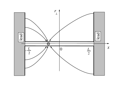
An explicit form of $U(x,x^{\prime})$ was found in Ref. [18] for realistic situation where the electrode surfaces are two planes $x=-L/2$ and $x=L/2$ perpendicular to the channel (Fig. 1). In this case

$$U(x,x^{\prime})=\frac{e^{2}}{\pi\epsilon}\,\int d^{2}q\,|\chi_{q}|^{2}\,G_{q}(x,x^{\prime}),$$ (3)

$\epsilon$ is the dielectric constant outside of the channel, $\chi_{q}$ is the Fourier-Bessel transform of the radial function $\chi({\bf r}_{\perp})$, and

                                                                           

$$G_{q}(x,x^{\prime})=\frac{L}{qL{\rm sinh}(qL)}\left\{\begin{array}[]{rcl}{\rm sinh}\left[q\left(L/2+x\right)\right]\,{\rm sinh}\left[q\left(L/2-x^{\prime}\right)\right]&{\rm if}&x<x^{\prime},\\ {\rm sinh}\left[q\left(L/2-x\right)\right]\,{\rm sinh}\left[q\left(L/2+x^{\prime}\right)\right]&{\rm if}&x>x^{\prime}.\\ \end{array}\right.$$ (4)

                                                                           

The interaction potential defined by Eqs. (3) and (4) is shown in Fig. 2 as a function of $x$ for a variety of $x^{\prime}$, with $V(x,x^{\prime})$ being a normalized form of $U(x,x^{\prime})$:

$$V(x,x^{\prime})=U(x,x^{\prime})\,\epsilon L/e^{2}\,.$$

FIG. 2.: Distance dependence of the electron-electron interaction potential for a variety of $x^{\prime}$. Dotted line is the envelope of $V(x,x)$ maxima.

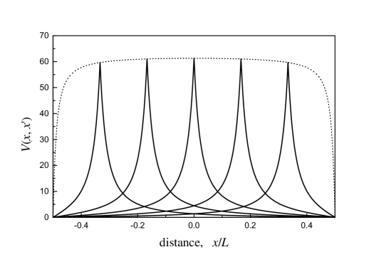
When the interelectron distance is larger than the wire radius $a$ ($|x-x^{\prime}|\gg a$), the potential decreases as $V\sim L/|x-x^{\prime}|$. In the middle part of the quantum wire $V(x=x^{\prime})\sim L/a$. Near the contacts ($x,x^{\prime}\to\pm L/2$), $V$ goes to zero due to screening effect of the charges induced on the lead surfaces. The behavior of this kind is quite general for the interaction potential regardless of the specific configuration of the leads. The potential defined by Eqs. (3) and (4) will be used below in getting an exactly solvable model of the interacting electron transport.

III The equation of motion

To study a linear response of the quantum wire structure to an external voltage $V_{a}\exp(-i\omega t)$ applied across the leads, we can restrict ourselves to the consideration of low-energy excitations of the electron system. The most adequate method for this purpose is the standard bosonization technique. [2, 3] We will use this technique assuming that the electron density fluctuations are long-range ones.

When external voltage is applied across the electrodes, the electric potential $\varphi(\bf r)$ in the wire is determined by the Poisson equation with the boundary conditions controlled by the applied voltage: $\varphi=0$ at the left reservoir and $\varphi=V_{a}$ at the right reservoir. It is convenient to present the electric potential in the wire as a sum

$$\varphi=\varphi_{\rm ext}+\varphi_{i}\,.$$ (5)

Here $\varphi_{\rm ext}$ is the potential which would be without the wire. It is determined by the Laplace equation with the same boundary conditions as the total potential $\varphi$. The potential $\varphi_{i}$ is defined by the Poisson equation with zero boundary conditions. The potential $\varphi_{i}$ is precisely the one used in Sec. II while calculating the electron-electron interaction energy [see Eqs. (2) and (3)].

Thus the bosonized Hamiltonian [3, 19] of 1D spinless electrons can be taken in the form

                                                                           

$$H=\int\!\frac{dx}{2\pi}\,v_{F}\!\left[(1\!+\!g_{1})\pi^{2}\Pi^{2}+(1\!-\!g_{1})\left(\partial_{x}\Phi\right)^{2}\right]-e\int dx\,\rho(x,t)\varphi_{\rm ext}(x,t)+\!\int\!\!\!\int\!\frac{dx\,dx^{\prime}}{2\pi^{2}}\,(\partial_{x}\Phi)\,U(x,x^{\prime})\,(\partial_{x^{\prime}}\Phi)\,,$$ (6)

where $\Phi(x,t)$ is the phase field related to the charge excitations, $\Pi(x,t)$ is the momentum density conjugate to $\Phi$, $v_{F}$ is the Fermi velocity, and $g_{1}$ is the backscattering parameter. [19]

By writing this Hamiltonian, we assume implicitly that the ground state is uniform. More careful investigation [20] shows that really the ground state is nonuniform due to two factors: (i) charging of the quantum wire which occurs as a consequence of the electron transfer between the wire and the reservoirs during the process of the establishment of the equilibrium electrochemical potential and (ii) Friedel oscillations near the contacts. The charge stored in the wire depends on the wire radius and the background density of the positive charge. This charge may be both positive and negative. Under certain conditions the wire remains neutral. The charging effect will be investigated elsewhere. In the present paper the ground state is assumed to be neutral. The Friedel oscillations of the electron density have a characteristic length of the order of the Fermi wavelength. Since we restrict our consideration by the long-range variation of the electron density, the ground state may be considered as uniform.

The long wave component of the electron density $\rho$ is related to $\Phi$ by

$$\rho=-\frac{1}{\pi}\>\partial_{x}\Phi\;.$$

From the Hamiltonian (6) we get the following equation of motion for the phase field $\Phi$:

$$\partial_{t}\left(\frac{1}{v\tilde{g}}\partial_{t}\Phi\right)-\partial_{x}\left(\frac{v}{\tilde{g}}\partial_{x}\Phi\right)=\partial_{x}\left[e\>\varphi_{\rm ext}+\frac{1}{\pi}\,\int\limits_{-L/2}^{L/2}dx^{\prime}\,U(x,x^{\prime})\,\partial_{x^{\prime}}\Phi\right]\;,$$ (7)

                                                                           

with

$$v=v_{F}\sqrt{1-g_{1}^{2}}\;,\qquad\qquad\tilde{g}=\sqrt{\frac{1+g_{1}}{1-g_{1}}}\;.$$

Following Refs. 4-6, we extend the one-dimensional Eq. (7) to the reservoirs assuming that the electron density inside them is extremely high and their conductivity is ideal. In such a case, $\varphi_{\rm ext}$ is a constant inside the reservoirs. Hence the first term on the right-hand side of Eq. (7) can be omitted. The second term (appearing from the electron-electron interaction energy $W$) is known to be small as compared with the kinetic energy on the left-hand side of Eq. (7) when the electron density is high. In this sense, the electrons in the reservoirs are noninteracting although the external field is of course ideally screened there. Thus, the right-hand side of Eq. (7) may be dropped in the reservoirs. The solution of the bosonized equation in the reservoirs should satisfy the condition that the density wave be restricted at $|x|\to\infty$ when the external voltage is turned on adiabatically. The boundary conditions at the contacts between the wire and the leads require the continuity of $\Phi$ and the particle current. The latter means that $(v/\tilde{g})\partial_{x}\Phi$ must be continuous there.

We find the exact solution of Eq. (7) with the electron-electron interaction potential $U(x,x^{\prime})$ defined by Eqs. (3) and (4). In terms of dimensionless variables

$$\xi=\frac{x}{L}\>,\qquad u=\frac{v\,\Phi}{e\tilde{g}LV_{a}}\>,\qquad f=\frac{\varphi_{\rm ext}}{V_{a}}\>,$$

Eq. (7) takes the form:

$$\frac{d}{d\xi}\left[\frac{du}{d\xi}+\beta\hat{V}\frac{du}{d\xi}-f(\xi)\right]\,+\,\Omega^{2}u\,=\,0\>.$$ (8)

Here

$$\beta=\frac{e^{2}\tilde{g}}{\pi\,\epsilon\,v}\>,\qquad\qquad\Omega=\frac{\omega L}{v}\>,$$

the operator $\hat{V}$ is defined as

$$\hat{V}\psi=\int\limits_{-1/2}^{1/2}d\xi^{\prime}\>V(\xi,\xi^{\prime})\>\psi(\xi^{\prime})\>,$$ (9)

where

                                                                           

$$V(\xi,\xi^{\prime})=2\,\int\limits_{0}^{\infty}\frac{dy}{{\rm sinh}y}\,|\chi_{y}|^{2}\>\left\{\begin{array}[]{rcl}{\rm sinh}\left[y\left(1/2+\xi\right)\right]\,{\rm sinh}\left[y\left(1/2-\xi^{\prime}\right)\right]&{\rm if}&\xi<\xi^{\prime},\\ {\rm sinh}\left[y\left(1/2-\xi\right)\right]\,{\rm sinh}\left[y\left(1/2+\xi^{\prime}\right)\right]&{\rm if}&\xi>\xi^{\prime}.\\ \end{array}\right.$$ (10)

                                                                           

The electron density in standard units is related to $u_{\xi}$ by

$$\rho(\xi)=-\frac{2\,e\,\tilde{g}\,V_{a}}{h\,v}\,u_{\xi}(\xi)\;.$$ (11)

After solving Eq. (8) in the reservoirs we use the continuity of the electron flow and the phase $\Phi$ at the contacts to obtain the boundary conditions directly to Eq. (8) in the inner region of the quantum wire, $-1/2\leq\xi\leq 1/2$,

$$u_{\xi}\,\pm\,i\,\Omega\tilde{g}\,\left.u\right|_{\xi=\mp 1/2}\,=\,0\;.$$ (12)

The integro-differential equation of the form Eq. (8) may be solved via an expansion in terms of the eigenfunctions of the operator $\hat{V}$. It is easy to verify that the functions

$$\psi_{n}(\xi)=\sqrt{2}\sin\left[\pi n\left(\xi+\frac{1}{2}\right)\right]\>,\qquad n=1,2,3,\dots\>,$$

are the eigenfunctions of $\hat{V}$ defined by Eqs. (9) and (10) with the eigenvalues

$$\lambda_{n}=2\int_{0}^{\infty}\frac{y\,dy}{y^{2}+(n\pi)^{2}}\;|\chi_{y}|^{2}\;.$$ (13)

For the geometry of the sample under consideration, the external potential $f(\xi)$ is a linear function which may be expanded in terms of $\psi_{n}(\xi)$ with even $n$.

The exact solution of Eq. (8) with the boundary conditions (12) can be obtained via the expansion in terms of $\psi_{n}(\xi)$. As a result, we get the following expressions for the dimensionless electron density $u_{\xi}(\xi)$:

$$u_{\xi}(\xi)\,=\,\sum_{n=1}^{\infty}c_{n}\sin\left[2\pi n(\xi+1/2)\right]\,$$ (14)

and the phase field $u(\xi)$,

$$u(\xi)\,=\,A(\Omega)-\sum_{n=1}^{\infty}\frac{c_{n}}{2\pi n}\cos\left[2\pi n(\xi+1/2)\right]\,,$$ (15)

where

$$c_{n}=B(\Omega)\>\frac{4\pi n}{4\pi^{2}n^{2}(1+\beta\lambda_{2n})-\Omega^{2}}\,,$$ (16)

$$A(\Omega)=\frac{1}{\Omega}\>\frac{1-4i\tilde{g}\Omega D(\Omega)}{2i\tilde{g}+\Omega-4i\tilde{g}\Omega^{2}D(\Omega)}\,,$$ (17)

$$B(\Omega)=\frac{-2i\tilde{g}}{2i\tilde{g}+\Omega-4i\tilde{g}\Omega^{2}D(\Omega)}\>,$$ (18)

$$D(\Omega)=\sum_{n=1}^{\infty}\frac{1}{4\pi^{2}n^{2}(1+\beta\lambda_{2n})-\Omega^{2}}\,.$$ (19)

IV Electron density distribution

The purpose of this section is to clarify how the real Coulomb interaction affects the value and the distribution of the charge density in the quantum wire structure.

First of all, let us consider a limiting case of the short-range interaction. In this case, $V(x,x^{\prime})\propto\delta(x-x^{\prime})$ and hence the eigenvalues are independent of $n$ and $\lambda_{2n}=\lambda$. All the sums are easily calculated, which results in the following expression for the normalized electron density:

$$u_{\xi}(\xi)=\frac{1}{\Omega\sqrt{1+\beta\lambda}}\>\frac{g^{*}\sin(\Omega^{*}\xi)}{g^{*}\cos(\Omega^{*}/2)-i\sin(\Omega^{*}/2)},$$ (20)

where renormalized values $g^{*}=\tilde{g}/\sqrt{1+\beta\lambda}$ and $\Omega^{*}=\Omega/\sqrt{1+\beta\lambda}$ are introduced. The density $\rho(\xi)$ calculated according to Eq. (20) coincides exactly with that found in Ref. [16] in the framework of the standard LL model with the interaction parameter $g=g^{*}$.

In the limit of $\Omega\to 0$, Eq. (20) yields

$$u_{\xi}(\xi)=\frac{\xi}{1+\beta\lambda}\>.$$ (21)

With increasing, frequency the charge waves appear which have resonances [16] along the wire when $\Omega=2\pi n\sqrt{1+\beta\lambda}$.

Another case will be useful in what follows as a reference point to demonstrate the Coulomb interaction effect. It is the case of noninteracting electrons which corresponds to $\beta=0$ in Eqs. (20) and (21).

For the case of the realistic interaction, the electron density distribution given by Eq. (14) is generally more complicated. However, simple results are obtained for the regions near the contacts and in the middle part of the wire, taking into account the specific behavior of $\lambda_{n}$ versus $n$. It is determined by the fact that the radial function $\chi({\bf r}_{\perp})$ is located in the region of radius $a$ which is much shorter than the wire length $L$, i.e., $\alpha=a/L$ is a small parameter. The results which will be given below are qualitatively valid for any localized function $\chi({\bf r}_{\perp})$. To be specific, we will use the Gaussian form for $\chi({\bf r}_{\perp})$ when it is necessary to bring the calculations to final form. One obtains that $\lambda_{n}$ varies slowly with $n$ for $\pi\alpha n\ll 1$ and $\lambda_{n}$ decreases as $n^{-2}$ for $\pi\alpha n\gg 1$.

In the vicinity of the contacts, the main contribution to the sum in Eq. (14) is due to the large-$n$ terms for which an asymptotic expression of $\lambda_{n}\sim n^{-2}$ can be used. Thus the following expression for the normalized electron density is obtained in the vicinity of the left electrode [$(1/2+\xi)\ll 1$]:

$$u_{\xi}(\xi)\approx-\frac{B(\Omega)}{2}\frac{\sinh(\xi\sqrt{2\beta/\alpha^{2}-\Omega^{2}})}{\sinh(\sqrt{2\beta/\alpha^{2}-\Omega^{2}}/2)}\,,$$ (22)

with $B(\Omega)$ being defined by Eq. (18). Equation (22) shows that (i) $u_{\xi}$ decreases with the distance from the contact as $\sinh(x/\ell)$, with characteristic length being

$$\ell\,=\,\frac{a}{\sqrt{2\beta-\alpha^{2}\Omega^{2}}}\;,$$

(ii) at $\Omega=0$, the boundary value of $u_{\xi}$ is equal to 1/2 and is independent of the interaction. [18]

In the middle part of the wire, Eq. (14) may be simplified when $\alpha$ is exponentially small, i.e., $-\ln\alpha\gg 1$. In this case the sum in Eq. (14) may by estimated assuming

$$\lambda_{n}\approx\lambda_{0}\equiv-\ln(2\pi^{2}\alpha^{2})-\gamma\,,$$

$\gamma\approx 0.57721\dots$ being Euler’s constant. This calculation results in the same equation as Eq. (20) for the short-range interacting electron gas, where $\lambda$ should be replaced by $\lambda_{0}$. This is equivalent to introducing an effective interaction parameter

$$g_{\rm eff}\approx\,\frac{\tilde{g}}{\sqrt{1+\beta\lambda_{0}}}$$

into the LL model.

For the sake of simplicity, we suppose $\tilde{g}=1$ below.

FIG. 3.: Distribution of the dc electron density $\rho$ (thick solid line) and the potential $\varphi$ (thin solid line) along the wire for long-range Coulomb interaction. The dashed line is the density distribution according to the LL model with $g_{\rm eff}$, the dotted line is that for noninteracting electrons. The parameters used are: the Fermi energy $\varepsilon_{F}=5$ meV and $\alpha=0.02$. The interaction parameter $\beta$ was calculated to be 0.35.

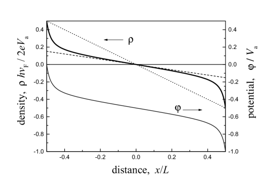
The effect of the Coulomb interaction on the electron density distribution in the quantum wire is demonstrated by Fig. 3 for the dc condition when a positive potential is applied to the left electrode with respect to the right one. Under the action of the external electric field, the electron system in the quantum wire is polarized: the electron liquid is compressed in the left part of the wire and decompressed in the right one. Respectively, at the left end of the quantum wire the excessive electrons appear while at the right end the electron density is decreased. If the electron-electron interaction is omitted [see the dotted line in Fig. 3 and Eq. (21) with $\beta=0$], the electron density decreases linearly with the distance, with the boundary value of the normalized density being equal to $\pm 1/2$. When the short-range interaction with the effective interaction parameter $g_{\rm eff}$ is turned on, the density distribution remains linear (dashed line). But the slope goes down as a result of a decrease in the electron liquid compressibility. Note that the boundary value of the electron density also decreases.

When the actual Coulomb interaction is turned on, the electron density distribution is changed qualitatively (thick line in Fig. 3). As compared with the noninteracting case, the charge density in the middle part of the wire decreases, which may be interpreted as neutralization of the negative and positive charges due to their mutual attraction. Towards the contacts the charge density increases reaching $\pm 1/2$ at the boundaries. This behavior may be understood from the fact that near the contacts the charges in the wire are neutralized by the image charges in the electrodes.

On the other hand, if we compare the Coulomb interaction case with the short-range interaction model, we find that the actual Coulomb interaction leads to an increase of the electron density fluctuation near the contacts. This fact may be interpreted as a result of the decrease in the interaction parameter $g$ due to screening the electron-electron interaction by the electrode.

At finite frequency, this near-contact effect of the Coulomb interaction is preserved up to a characteristic frequency $\Omega_{w}=\sqrt{2\beta}\,/\alpha$, above which the exponentially decreasing part of $\rho(x)$ disappears.

The electric potential $\varphi$ is easily calculated using Eq. (5), Green function (4), and the electron density $\rho(\bf r)$ found above. Distribution of $\varphi(\xi)$ along the quantum wire is shown in Fig. 3. A good proportionality is found between $\rho$ and $\varphi$ for dc conditions when $a/L\ll 1$:

$$\rho(\xi)\approx{\rm const}+\frac{\tilde{g}}{\pi v}e\varphi(\xi)\,.$$

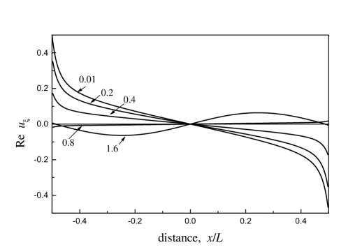
The main effect observed when the frequency grows is the appearance of the traveling charge waves. This is illustrated by Fig. 4, where the real part of the normalized electron density is shown as a function of the distance for a number of frequencies. The curves shown in Fig. 4 were obtained by numerical calculation of Eq. (8). [21] The frequency is given in a normalized form

$$\nu=\frac{\omega L}{2\pi v_{F}}$$

as labels to the curves.

FIG. 4.: Electron density distribution along the wire for a set of frequencies. The curves are labeled by the normalized frequency $\nu$. The parameters used in the calculations are the same as in Fig. 3.

Our analytical solution given by Eqs. (14) and (16) shows that there is a set of characteristic frequencies $\Omega_{n}$ which are determined by the poles of $D(\Omega)$:

$$\Omega_{n}=2\pi n\sqrt{1+\beta\lambda_{2n}}\,.$$ (23)

For $\Omega=\Omega_{n}$, the electron density is a standing wave with zeros at the contacts, $n$ being the wave number:

$$\left(\frac{du}{d\xi}\right)_{n}\propto\frac{\sin\left[2\pi n(\xi+1/2)\right]}{4\pi n(1+\beta\lambda_{2n})}\,.$$

It is noteworthy that the electron flow turns to zero at the contacts simultaneously with the electron density. Thus $\Omega_{n}$ is the resonant frequencies of the charge waves in the quantum wire. Under the resonant condition the electron density perturbation is locked inside the wire.

Equation (23) shows that the frequency $\Omega_{n}$ depends on the wave number $2\pi n/L$ in a nonlinear manner due to the dependence of $\lambda_{n}$ upon $n$. For $n\to\infty$, the resonant frequency is proportional to the wave number which corresponds to the soundlike dispersion. For low wave numbers [$n\leq(\pi\alpha)^{-1}$], $\Omega_{n}$ is noticeably higher than one expects from the soundlike dispersion.

It is instructive to compare Eq. (23) with the dispersion equation for charge waves in an infinite quantum wire which was found by Schulz [19] using the bosonization technique,

$$\Omega(p)=p\sqrt{1+\beta V_{p}}\,,$$ (24)

where $p$ is the wave vector normalized by $L^{-1}$ and $V_{p}$ is the Fourier transform of the interaction potential, which is approximated by the modified Bessel function $K_{0}(\alpha p)$. A similar dispersion law was obtained by Das Sarma and Hwang [22] for 1D plasmons in the long-wavelength limit in the frame of the random-phase approximation taking into consideration the more general form of the interaction potential. Equation (24) differs from Eq. (23) in the replacement $\lambda_{2n}$ by $V_{p}$. A reasonable approximation for $\lambda_{2n}$ is

$$\lambda_{2n}\approx\exp\left(2\pi^{2}\alpha^{2}n^{2}\right)\,E_{1}\left(2\pi^{2}\alpha^{2}n^{2}\right)\,,$$ (25)

where $E_{1}(z)$ is the exponential integral. It is worth noting that in the limit $L\to\infty$, Eq. (25) is the same as the Fourier transform of the interaction potential used in Ref. [17] when the screening length is much larger than the quantum wire diameter. On setting $p=2\pi n$ and comparing the expressions (23) and (24), one can see that they are close when $\pi\alpha n\ll 1$ and differ significantly in the opposite case.

One can say that Eq. (23) is a discrete version of the dispersion relation for 1D electrons which takes correctly into account the electron-electron interaction in a finite 1D system. It will be shown below that the discrete character of the resonant frequencies $\Omega_{n}$ of finite quantum wire results in strong peculiarities of the frequency dependence of admittance.

V The impedance

The electron current in a quantum wire is determined by the time derivative of the phase field. [3] In the terms of the normalized phase $u$, the current is

$$j(x,\omega)=-\frac{2i\omega e^{2}\tilde{g}L}{hv}\,u(x,\omega)\,V_{a}\,.$$ (26)

The current calculated in such a way depends on the coordinate $x$ along the wire. However, the electric current $j_{\rm meas}$ which is detected by a measuring device is obviously independent of $x$. This current is defined as a charge flow through the leads. Its formation process is analyzed in Appendix A as applied to the specific quantum wire structure considered here. The measured current is the sum of a trivial capacitance current and the current caused by the quantum wire presence. According to the Shockley theorem, [23] the latter is

$$j_{\omega}=\frac{1}{L}\int_{-L/2}^{L/2}\!dx\,j(x,\omega)\,.$$

Due to Eqs. (15) and (26), the current $j_{\omega}$ becomes

$$j_{\omega}=i\frac{e^{2}}{h}\,2\tilde{g}\,A(\Omega)\,V_{a}\,,$$

with $A(\Omega)$ being defined by Eq. (17). This results in the following expression for the quantum wire structure impedance:

$$Z(\Omega)=\frac{h}{e^{2}}\left[\frac{1}{1-4i\tilde{g}\Omega D(\Omega)}-\frac{i\Omega}{2\tilde{g}}\right]\,.$$ (27)

In what follows, the impedance is analyzed rather than the admittance which is usually considered, because the frequency dependence of the impedance shows more pronounced features caused by the charge waves. The real part of $Z$ is

$${\rm Re}Z=\frac{h}{e^{2}}\>\frac{1}{1+[4\tilde{g}\Omega D(\Omega)]^{2}}\,.$$ (28)

When $\Omega\to 0$, the impedance is equal to $h/e^{2}$ and is independent of the interaction parameter $\beta$. The frequency dependence of ${\rm Re}Z$ is mainly governed by that of $D(\Omega)$. The resonant frequencies $\Omega_{n}$ are by definition the poles of $D(\Omega)$. Between the neighboring poles, there is a zero of $D(\Omega)$. Equation (28) shows that ${\rm Re}Z=0$ when $|D|\to\infty$ and ${\rm Re}Z=h/e^{2}$ when $D\to 0$. Thus with increasing frequency, ${\rm Re}Z$ oscillates between zero (which occurs at the resonant frequencies) and $h/e^{2}$, these limiting values being independent of the interaction. The frequency dependence of ${\rm Re}Z$ is illustrated by Fig. 5, where three cases are compared: noninteracting electrons, the LL model with short-range interaction, and the electrons with actual Coulomb interaction.

FIG. 5.: Real part of the impedance versus the normalized frequency $\nu$ for true long-range interaction (—), LL approach with $g$=0.63 (- - -), and noninteracting electrons ($\cdots$).

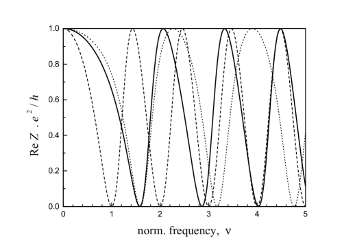
An interesting result is that ${\rm Re}Z=0$ for the resonant frequencies. Under resonant condition the time-dependent evolution of the electron density is essentially oscillations between the two ends of the wire, and electrons are not emitted/absorbed by the contacts. As a consequence, the electric current component in-phase with the applied voltage vanishes, and the real part of both the admittance and the impedance turns to zero. However, in reality there is a finite dissipation which was not taken into account. The inclusion of the dissipation into calculations should restrict the minimum of ${\rm Re}Z$ by some low value.

The resonances of ${\rm ReZ}$ occur when the frequency is a multiple of the inverse time of flight of electron excitations along the quantum wire. This conclusion was confirmed for both the noninteracting [24, 25] electrons and the short-range interacting electrons in the LL model. [16] The fact that in the case of the Coulomb interaction the impedance oscillations are nonperiodic may be interpreted as a result of the frequency-dependent renormalization of the charge-wave velocity due to the Coulomb interaction. At low frequency, the velocity renormalized by the Coulomb interaction is essentially larger than $v_{F}$. The resonance frequency spectrum shows that the velocity decreases with frequency. It is worthwhile to note that the phase velocity is important since the resonant conditions are obviously related to the wave interference.

The imaginary part of the impedance may be presented in the form

$${\rm Im}Z=-\omega L_{\rm eff}+\frac{h}{e^{2}}\>\frac{4\tilde{g}\Omega D(\Omega)}{1+[4\tilde{g}\Omega D(\Omega)]^{2}}\,,$$ (29)

where

$$L_{\rm eff}=\,\frac{hL}{2e^{2}v_{F}}\,.$$

FIG. 6.: Imaginary part of the impedance versus the normalized frequency $\nu$.

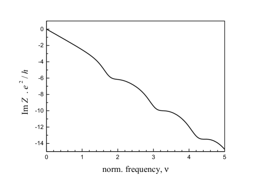
The frequency dependence of ${\rm Im}Z$ consists in the linear decrease caused by the first term in the brackets and oscillations around this dependence due to the second term. This behavior is illustrated by Fig. 6. The linear dependence of the ${\rm Im}Z$ on the frequency is obviously dominating, which allows one to interpret $L_{\rm eff}$ as a frequency-independent inductance. [16]

When the frequency is small, the second term on the right-hand side of Eq. (29) is comparable with the first one. In this case we can expand Eq. (29),

$${\rm Im}Z=\frac{h}{e^{2}}\,\frac{\Omega}{2\tilde{g}}\>\left[-1+\frac{2\tilde{g}^{2}}{\pi^{2}}\sum_{n=1}^{\infty}\frac{1}{n^{2}(1+\beta\lambda_{2n})}\right]\,,$$

to estimate the second term. If the electron-electron interaction is omitted ($\beta=0$, $\tilde{g}=1$), the second term is equal to 1/3. Upon increasing $\beta$, the second term decreases and ImZ remains negative in spite of the fact that the backscattering parameter $\tilde{g}$ slightly increases when the interaction is turned on. Thus the reactive part of the impedance is always inductive if the electron-electron interaction is repulsive independent of the interaction strength.

The behavior of the impedance we have obtained here correlates with that found for the case of both the short-range interaction [16] and noninteracting electrons. [25] Somewhat different behavior of the impedance was found recently in Ref. [17] for a quantum wire without leads based on a rather general approach, which allows one to consider an arbitrary distribution of the external electric field along the quantum wire. In this case the impedance was shown to include both the inductive and capacitive components. This difference originates from the different experimental situation which was considered. In Ref. [17], a homogeneous wire of infinite length with a continuous spectrum of eigensolutions was examined which results in a dispersion relation $\omega=\omega(k)$. The resonant feature of the impedance is caused by the inflection point of $\omega(k)$ where the group velocity reaches a minimum, with the characteristic wavelength of the charge waves being of the order of the wire radius. In the present paper, we consider a more specific situation of a finite wire restricted by leads with a discrete spectrum of eigenfunctions. The resonances we have found are attributed to the finite length of the wire. They appear when the characteristic wavelength of the charge waves is of the order of the wire length, i.e., the frequency is much lower than the resonant frequency which appears in Ref. [17].

The total admittance of the quantum wire structure is formed by both the quantum wire impedance $Z$ defined by Eq. (27) and the interelectrode capacitance $C_{0}$ which is necessarily present there. Using Eq. (A.3) one obtains

$$Y_{\rm tot}(\omega)=\frac{1}{Z}-i\omega C_{0}=\frac{{\rm Re}Z-i({\rm Im}Z+\omega C_{0}|Z|^{2})}{|Z|^{2}}\,.$$ (30)

It is of interest to find the eigenfrequencies of the admittance (the impedance) which describe the behavior of the system under consideration as an element of electric circuit. They are known to be determined by the poles and zeros of the admittance (the impedance). The admittance zeros characterize the system when the external circuit is open while the poles correspond to the short-circuit case.

Equation (30) shows that the poles of $Y_{\rm tot}$ coincide with the zeros of $Z$ (or the poles of the quantum wire admittance). It follows from Eqs. (27) and (19) that there is only one set of eigenfrequencies which are complex with a negative imaginary part corresponding to decaying fluctuations. Several authors have found two sets of the eigenfrequencies in the case of short-range interacting electrons for a three-terminal structure [12] or using an other way for the calculation of the observed current. [15] Both sets of eigenfunctions also describe the decaying fluctuations.

Of more interest, in our opinion, are the zeros of $Y_{\rm tot}(\Omega)$. We show that in this case the conditions can be found under which the eigenfrequencies are real and charge-wave excitations are very slowly decaying. According to Eq. (30), $Y_{\rm tot}=0$ when two equations are satisfied simultaneously:

$${\rm Re}Z(\Omega)=0\,,$$ (31)

$${\rm Im}Z(\Omega)+\frac{\Omega vC_{0}}{L}\,|Z(\Omega)|^{2}=0\,.$$ (32)

The first equation is obviously satisfied by the set of real frequencies $\Omega_{n}$ defined by Eq. (23). The second equation can also be satisfied at one of frequencies $\Omega_{n}$ if the capacitance $C_{0}$ is appropriately fitted, for instance, via changing the lead areas. The resonant value of $C_{0}$ is estimated as

$$C_{0}\approx\frac{e^{2}L}{2\pi^{2}hv_{F}}.$$

Physically, Eq. (31) means the absence of dissipation while Eq. (32) is a resonant condition for the circuit which consists of the quantum wire inductance and the interelectrode capacitance. Under this condition, the resonant frequency of the charge waves in the wire coincides with that of the $L_{\rm eff}C_{0}$ circuit, which results in a strong increase of the charge-wave amplitude.

VI Conclusion

In this paper we have investigated the linear transport of interacting electrons in a quantum wire of mesoscopic length with massive leads. The key point is the full enough account of the actual Coulomb interaction inside the wire and of three-dimensional electric field in the surrounding media. The Coulomb interaction in a mesoscopic quantum wire includes both the direct interaction of electrons with each other and their interaction via the image charges induced on the leads. We have found an exact analytical solution of the problem. This has become possible due to (i) use of the bosonization technique which is well suited to consider the low-energy excitation of 1D interacting electrons, and (ii) solving the equation of motion for the bosonic phase field by expansion in terms of the eigenfunctions of the electron-electron interaction operator, which have been found for a model case where the electrodes are plates perpendicular to the wire.

We have found that the actual Coulomb interaction affects strongly the electron density distribution along the wire in comparison with that in the case of short-range interacting electrons in the conventional LL model. The nonlocal Coulomb interaction manifests itself first of all in the noticeable increase of the charge density in the vicinity of the contacts with leads. Here the electron density perturbation decreases exponentially with the distance from the contact. This effect is essential when the frequency is not too high ($\Omega<\alpha^{-1}\sqrt{2\beta}$).

Another effect of the Coulomb interaction is the renormalization of the charge-wave velocity. Namely, in contrast with the short-range LL model the long-range Coulomb interaction causes the frequency-dependent renormalization of the charge-wave velocity. This effect manifests itself in the frequency dependence of the real part of the impedance. With increasing frequency ${\rm Re}Z$ oscillates between two limiting values which are independent of the interaction. These are zero and $h/e^{2}$. The fact that ${\rm Re}Z$ becomes zero is related to the resonances of the charge waves along the wire length. Such resonances occur also when there is no long-range interaction. The Coulomb interaction causes the resonances to be nonequidistant in frequency, which means that the charge-wave velocity is frequency-dependent. At low frequency the charge-wave velocity is essentially larger than the Fermi velocity. With increasing frequency, the charge-wave velocity decreases and tends asymptotically to the Fermi velocity.

A The current being measured

The current $j_{\rm meas}$ being detected by the measuring device in the external circuit is equal to the charge flow in the leads. Since the currents in the left and right leads are obviously equal each other let us consider the current in the left electrode. It is equal to the sum of the charge flow through the wire $j(x=-L/2)$ and the charge stored at the lead surface per unit time:

$$j_{\rm meas}=\left.j\right|_{x=-L/2}+\frac{dQ_{s}}{dt}\,.$$ (A.1)

The charge $Q_{s}$ consists of two components. One is the external charge caused by the applied voltage if the wire is absent, $Q_{\rm ext}=C_{0}V_{a}$, with $C_{0}$ being the mutual capacity of the electrodes. The other component is the charge $Q_{\rm ind}$ induced by the charges located within the wire. The latter is determined as

$$Q_{\rm ind}=\int_{S}ds\,\sigma\,,$$

where

$$\sigma=-\frac{\epsilon}{4\pi}\frac{\partial\varphi({\bf r})}{\partial n}\,,$$

$\varphi$ is the potential of the charge distributed along the wire and $n$ is the outward normal to the lead surface. The potential $\varphi$ is expressed in terms of the charge density $\rho({\bf r})$ via the Green function $G({\bf r},{\bf r^{\prime}})$ of the Laplace equation with zero boundary conditions at the lead surfaces.

Direct calculation results in

$$Q_{\rm ind}=-e\int_{-L/2}^{L/2}dx^{\prime}\rho(x^{\prime},t)\left.\frac{\partial G_{q}(x,x^{\prime})}{\partial x}\right|_{x=-L/2,q=0}\,.$$

Using Eq. (4) and the continuity equation

$$\frac{\partial\rho}{\partial t}=-\frac{\partial j}{\partial x}\,,$$

we obtain the induced current

$$\frac{dQ_{\rm ind}}{dt}=-j(-\frac{L}{2},t)+\frac{1}{L}\int_{-L/2}^{L/2}dx^{\prime}j(x^{\prime},t)\,,$$ (A.2)

where $j(x,t)$ is the particle current in the wire.

Combining Eqs. (A.1) with (A.2) one obtains

$$j_{\rm meas}=\frac{1}{L}\int_{-L/2}^{L/2}dx^{\prime}j(x^{\prime},t)+C_{0}\frac{dV_{a}}{dt}\,.$$ (A.3)

The first term in equation (A.3) is a current induced by electrons moving in the wire, while the second one is a trivial capacitance current. Equation (A.3) is a particular case of the general Shockley theorem. [23] For arbitrary form and configuration of the leads the Shockley theorem is presented as follows

$$j_{\rm meas}=\frac{1}{V_{a}}\int_{-L/2}^{L/2}dx^{\prime}j(x^{\prime},t)F(x^{\prime})+C_{0}\frac{dV_{a}}{dt}\,,$$ (A.4)

where $V_{a}$ is the potential difference between the leads and $F(x)$ is the electric field along the electron trajectory due to $V_{a}$. According to the original derivation, [23] the field $F(x)$ appears here as a result of using the reciprocity theorem when calculating the charge induced in the leads by the charges moving along the wire. Thus, $F(x)$ has a sense of the external electric field which does not include the polarization of the 1D electron system.

Recently [26, 27] a question was discussed regarding which electric field determines the measured electric current in the quantum wire – the external field or the internal one – which depends on the polarization of 1D electrons. In this connection we note that in our case the current calculated according to Eq. (A.4) does not depend on what electric field is used. The internal electric field is defined by the right-hand side of Eq. (7), where the first term is the external field $F_{ext}$ and the second one is the induced field $F_{ind}$. It is easy to see using Eqs. (26), (14), and (15) that the integral of the product $j(x)F_{ind}(x)$ is zero:

$$\int\!\!\!\int_{-L/2}^{L/2}dx\,dx^{\prime}\,j(x,t)\frac{\partial V(x,x^{\prime})}{\partial x}\,\frac{\partial\Phi(x^{\prime})}{\partial x^{\prime}}\,=\,0\,.$$

Since in our case $F_{ext}$ is independent of $x$, the measured current can be found from Eq. (A.3).

REFERENCES

- [1] Electronic address: vas199@ire216.msk.su
- [2] F.D.M. Haldane, J. Phys. C 14, 2585 (1981).
- [3] J. Voit, Rep. Prog. Phys. 58, 977 (1995).
- [4] S. Tarucha, T. Honda, and T. Saku, Solid State Commun. 94, 413 (1995).
- [5] D.L. Maslov and M. Stone, Phys. Rev. B 52, R5539 (1995).
- [6] V.V. Ponomarenko, Phys. Rev. B 52, R8666 (1995).
- [7] I. Safi and H.J. Schulz, Phys. Rev. B 52, R17 040 (1995).
- [8] A. Yacoby, H.L. Stormer, N.S. Wingreen, L.N. Pfeiffer, K.W. Baldwin, and K.W. West, Phys. Rev. Lett. 77, 4612 (1996).
- [9] A. Yacoby, H.L. Stormer, K.W. Baldwin, L.N. Pfeiffer, and K.W. West, Solid State Commun. 101, 77 (1997).
- [10] L.I. Glazman, I.M. Ruzin, and B.I. Shklovskii, Phys. Rev. B 45, 8454 (1992).
- [11] R. Egger and H. Grabert, Phys. Rev. Lett. 79, 3463 (1997).
- [12] Ya.M. Blanter, F.W.J. Hekking, and M. Büttiker, Phys. Rev. Lett. 81, 1925 (1998).
- [13] M. Büttiker and T. Christen, in Quantum Transport in Semiconductor Submicron Structures, edited by B. Kramer, Vol. 326 of NATO Advanced Study Institute Series E (Kluwer, Dordrecht, 1996) pp. 263-291.
- [14] N.P. Sandler and D.L. Maslov, Phys. Rev. B 55, 13 808 (1997).
- [15] V.V. Ponomarenko, Phys. Rev. B 54, 10 328 (1996).
- [16] V.A. Sablikov and B.S. Shchamkhalova, Pis’ma Zh. Eksp. Teor. Fiz. 66, 40 (1997) [JETP Lett. 66, 41 (1997)].
- [17] G. Cuniberti, M. Sassetti, and B. Kramer, Phys. Rev. B 57, 1515 (1998).
- [18] V.A. Sablikov and B.S. Shchamkhalova, Pis’ma Zh. Eksp. Teor. Fiz. 67, 184 (1998) [JETP Lett. 67, 196 (1998)].
- [19] H.J. Schulz, Phys. Rev. Lett. 71, 1864 (1993).
- [20] V.A. Sablikov and S.V. Polyakov, unpublished.
- [21] V.A. Sablikov and S.V. Polyakov, Phys. Low-Dimens. Struct. 5/6, 101 (1998).
- [22] S. Das Sarma and E.H. Hwang, Phys. Rev. B 54, 1936 (1996).
- [23] W. Shockley, J. Appl. Phys. 2, 635 (1938).
- [24] B. Velicky, J. Masek, and B. Kramer, Phys. Lett. A 140, 447 (1989).
- [25] V.A. Sablikov and E.V. Chensky, Pis’ma Zh. Eksp. Teor. Fiz. 60, 397 (1994) [JETP Lett. 60, 410 (1994)].
- [26] A. Kawabata, J. Phys. Soc. Jpn. 60, 30 (1996).
- [27] Y. Oreg and A.M.Finkel’stein, Phys. Rev. B 54, R14 269 (1996).