Bosonization for Wigner-Jordan-like Transformation :
Backscattering and Umklapp-processes on Fictitious Lattice.

Abstract

We analyze the asymptotic behavior of the exponential form in the fermionic density operators as the function of ruling parameter $Q$. In the particular case $Q=\pi$ this exponential associates with the Wigner-Jordan transformation for $XY$ spin chain model. We compare the bosonization approach and the evaluation via the Toeplitz determinant. The use of Szegö-Kac theorem suggests that at $Q>\pi/3$ the divergent series for intrinsic logarithm provides a bosonized solution and faster decaying one, found as the logarithm’s value on another sheet of the complex plane. The second solution is revealed as umklapp-process on the fictitious lattice while originates from backscattering terms in bosonized density. Our finding preserves in a wide range of fermion filling ratios.

]

The method of bosonization proved to be an effective tool for studying the properties of one-dimensional (1D) systems of interacting fermions. Describing the fermion system through the bosonic collective modes, [1] this technique was initially used for providing the exact solution of Luttinger model. [2] Recently the bosonization attracted a renewed interest due to investigation of Quantum Hall Effect [3], two channel Kondo model [4] and High-$T_{c}$ superconductivity. [5] Essential efforts are made to generalize the method for higher dimensions. [6]

In a recent paper [7] the bosonization technique was successfully employed to study the magnetic properties of the high-$T_{c}$ -related system. The 1D model with a spin-charge separation was solved and important physical consequences were obtained. The bosonization was used to estimate the (time-dependent) Wigner-Jordan-like exponential in fermionic on-site density operators $c_{j}^{\dagger}c_{j}$. Namely the quantity of the interest was the average $\left\langle\exp\ iQ\sum_{j=1}^{l}c_{j}^{\dagger}c_{j}\right\rangle$ at arbitrary value of $Q$. This average should be $2\pi-$periodic in $Q$ and attain the real value at $Q=\pi$ (the case for Wigner-Jordan transformation). These properties are lost after the simple use of the bosonization technique. Although various ad hoc tricks were implemented to cure the problem at $Q=\pi$ (see, e.g. [8] and references therein), no systematic bosonic representation existed.

In an attempt to resolve this puzzle we addressed ourself to the vast available literature on the subject. The results of this survey could be outlined in the following way. The straightforward application of bosonization, though formally valid, is seemingly incapable to provide a closed form of the final answer due to the complexity of intermediate expressions. The key could be found in comparison of two counterparts for the same problem : the bosonization by Mattis and Lieb [2] and Luttinger’s original solution [9] via the Toeplitz determinants. The Szegö-Kac theorem, used in the approach by Luttinger, dates back [10] to Onsager famous solution of 2D Ising model. The exhaustive literature on the latter subject suggests some useful hints about the discussed issue.

Basing on the alternative representation of the considered average, we make a following major statement. The above exponential form in the fermionic density operator reveals a singularity at some finite value of $Q$. This is verified by an application of Szegö-Kac theorem and manifests itself as the appearance of umklapp-processes contribution on the fictitious lattice (see below). We provide an explicit expression obeying the above $2\pi$-periodicity and real valued at $Q=\pi$.

The rest of the paper is organized as follows. We formulate the simplified version of our problem and solve it by bosonization method in Section I. We rewrite our quantity of interest as the Toeplitz determinant and apply the Szegö-Kac theorem in Section II ; the appearing singularity is discussed here. In Section III the structure of the desired solution is suggested and justified. This solution and its physical consequences are discussed in the Section IV of the paper.

I The model and approach by bosonization

We consider a gas of free spinless fermions on a lattice with Hamiltonian

$$H_{1} = \sum_{p}(\cos k_{F}-\cos p)c^{{\dagger}}_{p}c_{p}$$ (1)

where Fermi wave-vector $k_{F}=c\pi$. Our aim is to evaluate a following quantity :

$${\cal C}(Q,l)=\left\langle\exp\ iQ\sum_{j=1}^{l}c_{j}^{\dagger}c_{j}\right\rangle_{H_{1}},$$ (2)

where $c_{j}^{\dagger}c_{j}$ corresponds to the on-site density operator. The expression of the form (2) appeared previously in various studies concerning the physics in one dimension. For the particular case of $Q=\pi$ it is found in the Wigner-Jordan transformation for the spin operators in 1D XY model. It can be also associated with the incorporation of interaction effects in the bosonization approach to Luttinger model. In our problem (see Appendix A for details) the quantity (2) connected the observable spin susceptibility and easier tractable one on the fictitious lattice. The parameter $Q$ appeared as a wave-vector belonging to the fictitious lattice and varied over the whole Brillouin zone, $Q\in[-\pi,\pi)$.

The average (2) is easily evaluated by introducing the boson representation for the fermionic density. The main steps of this derivation are outlined below. First we introduce the density operator :

$$\rho(q)=N^{-1}\sum_{p}c^{\dagger}_{p}c_{p+q},$$ (3)

where $N$ is the total number of lattice sites.

$${\cal C}(Q,l)=e^{iQcl}\left\langle\exp\left[iQ\sum_{q}\phi(q,l)\rho(q)\right]\right\rangle,$$ (4)

and we have defined $\phi(l,q)=(1-e^{iql})/(1-e^{iq})$ and $\phi(l,0)=l$. The non-fluctuating component of the density $\langle c_{j}^{\dagger}c_{j}\rangle=c$ is treated separately and leads to the prefactor $e^{iQcl}$ in Eq.  4.

Now we may use a well known procedure[11] in which the fermion density is split into contributions from right and left moving fermions. We write

$$\rho(q) = \rho_{+}(q)+\rho_{-}(q)$$ (5)

$$= N^{-1}\sum_{p>0}c^{\dagger}_{p}c_{p+q}+N^{-1}\sum_{p<0}c^{\dagger}_{p}c_{p+q},\quad q\neq 0$$ (6)

$$\rho(q) = N^{-1}(N_{-}+N_{+}),\quad q=0$$ (7)

where $N_{+}$ ($N_{-}$) are charge operators for right (left) movers, describing the fluctuations of the Fermi surface [12]

The long wave-length density fluctuations of the $1\!-\!d$ electron gas may be represented by boson operators defined by the relations :

$$\begin{array}[]{l}\rho_{+}(q)=v(q)\left(\theta(q)b_{q}^{\dagger}+\theta(-q)b_{-q}\right)\\ \rho_{-}(q)=v(q)\left(\theta(q)b_{-q}+\theta(-q)b_{q}^{\dagger}\right),\end{array}$$ (10)

where $v(q)=\sqrt{|q|/(2N\pi)}$. [2] In terms of the above operators, the Hamiltonian reads :

$$H=v_{F}\sum_{q}|q|b_{q}^{\dagger}b_{q}+v_{F}\frac{\pi}{N}(N_{+}^{2}+N_{-}^{2})$$ (11)

where Fermi velocity $v_{F}=\sin k_{F}$.

With these definitions we may rewrite Eq. 4 in the form :

$${\cal C}(Q,l) = e^{iQcl}\left\langle\exp i\frac{Ql}{N}(N_{+}+N_{-})\right\rangle$$ (13)

$$\times\left\langle\exp iQ\sum_{q}v(q)\phi(q,l)\left[b_{q}^{\dagger}+b_{-q}\right]\right\rangle$$

Let us focus on the case of zero temperature; the finite $T$ are considered in the Appendix B. The fermionic vacuum corresponds then to the absence of bosons in the ground state, in addition $N_{\pm}=0$. The evaluation of the above expression yields immediately :

$${\cal C}(Q,l)=\exp\left[iQcl-\frac{Q^{2}}{2\pi^{2}}{\cal F}(l)\right],$$ (14)

where

$${\cal F}(l)=\pi^{2}\sum_{q}v^{2}(q)\frac{1-\cos q(l-l^{\prime})}{1-\cos q}.$$ (15)

The integration in Eq. 15 is cutoff at a wavevector of order $k_{F}$ since the density fluctuations of the electron gas are well defined excitations only in the region $|q|\lesssim k_{F}$. [13]

Evaluating the above integral in the logarithmic approximation we find :

$${\cal C}(Q,l)\propto{\cal C}_{boson}(Q,l)=\exp\left[iQcl-\frac{Q^{2}}{2\pi^{2}}\ln l\right],$$ (16)

This expression indicates the power law decay of the correlations with $l$, which is well established fact for the 1D systems. [14]

The result (16) seems however unsatisfactory on two following reasons. First, the initial expression (2) was invariant under the shift $Q\to Q+2\pi$. This property is obviously absent in (16). Second, $e^{i\pi c_{j}^{\dagger}c_{j}}=\pm 1$ for each $j$, and one should have the real value of (2) at $Q=\pi$, meanwhile this feature is also not found in (16).

The inadequacy of the expression (16) for the particular case $Q=\pi$ was noticed by Luther and Peschel [11]. They argued that the term $\propto e^{-iQcl}$ should be added to (16) to get the correct result. The necessity of inclusion of such term was ascribed to the $2k_{F}$ (“backscattering”) processes ( we remind that $2k_{F}=2\pi c$ and $Qc-2k_{F}=-Qc$). Really, one might argue that the representation (6) of the electronic density is incomplete and the low-energy fluctuations with $q\simeq 2k_{F}$ should be explicitly included into the notation. [12] These terms are described in the Appendix C where we show that the “$2k_{F}$” terms produce very complicated and seemingly intractable expressions.

A general question arises here. If $2k_{F}$ processes provide the real value of ${\cal C}(Q,l)$ at $Q=\pi$, then why these $2k_{F}$ terms are less important at other values of independent parameter $Q$ where ${\cal C}(Q,l)$ is not real ? Below we argue that at $Q>\pi/3$ the “marginal” contribution of backscattering breaks the analiticity of ${\cal C}(Q,l)$.

In our problem the parameter $Q$ varies from 0 to $\pi$. Therefore the ignorance of the above discrepancy might produce non-trivial consequences. To resolve this question we formulate below the alternative way for the evaluation of ${\cal C}(Q,l)$ (2) and provide the answer which explicitly obeys two above conditions, the $2\pi$-periodicity in $Q$ and real valued quantity ${\cal C}(Q=\pi,l)$.

II Szegö-Kac theorem

We use a modification of an approach originally due to Lieb, Schultz and Mattis [15]. It is based on a representation of the correlation function ${\cal C}(Q,l)$ of Eq. (4) as the Toeplitz determinant

$${\cal C}(Q,l) = det(M^{(l)})$$ (17)

$$M_{km}^{(l)} = \delta_{km}-(1-e^{iQ})g_{km}.$$ (18)

The $l\!\times\!l$ matrix $M^{(l)}$ is constructed out the fermionic correlation functions

$$g_{km} = \langle c_{k}^{\dagger}c_{m}\rangle=\frac{1}{2\pi}\int_{-\pi}^{\pi}dq\,n_{q}e^{iq(k-m)}$$ (19)

$$= \frac{\sin(\pi c(k-m))}{\pi(k-m)}$$ (20)

where the Fermi function $n_{q}=1$ at $|q|<k_{F}$ and $n_{q}=0$ otherwise.

For completeness we sketch below the derivation of (17). We observe that

$$e^{iQc_{i}^{\dagger}c_{i}}=(c_{i}^{\dagger}+c_{i})(c_{i}^{\dagger}+e^{iQ}c_{i})$$ (21)

which is readily verified in the representation diagonalizing $c_{i}^{\dagger}c_{i}$. Defining

$$A_{i}=c_{i}^{\dagger}+c_{i},\quad B_{i}=c_{i}^{\dagger}+e^{iQ}c_{i},$$ (22)

we have

$${\cal C}(Q,l) = \langle A_{1}B_{1}A_{2}\ldots B_{l-1}A_{l}B_{l}\rangle$$ (23)

Zuber and Itzykson evaluated the square of the value (2) in a similar problem.[16] They noticed at $Q=\pi$ one had the possibility to identify the operators $A_{i},B_{i}$ with a new fermionic (Majorana) field. This is not so for other values of $Q$ since $A_{i}B_{i}+B_{i}A_{i}=1+e^{iQ}\neq 0$, therefore the trick used in [16] with introducing the second Majorana field is hardly applicable to our case.

However one can apply the Wick theorem which permits one to express the vacuum expectation value (23) in terms of expectation values of products of just two operators. [17] This procedure is facilitated if one notices that

$$\langle A_{i}A_{j}\rangle=\langle B_{i}B_{j}\rangle=0,\quad i\neq j$$ (24)

and

$$\langle A_{i}B_{j}\rangle=\delta_{ij}-(1-e^{iQ})g_{ij}$$ (25)

The most straightforward contribution to (23) is

$\displaystyle\langle A_{1}B_{1}\rangle\langle A_{2}B_{2}\rangle\ldots\langle A_{l}B_{l}\rangle$

All other pairings are obtained by permuting the $B$’s among themselves with $A$’s fixed. [18] The number of crossings of $A$’s by $B$’s is always even, hence the sign associated with a given permutation is $(-1)^{p}$ where $p$ is the signature of the permutation $P$ of the $B$’s. As a result

$${\cal C}(Q,l) = \sum_{P}(-1)^{p^{\prime}}\langle A_{1}B_{P(1)}\rangle\langle A_{2}B_{P(2)}\rangle\ldots\langle A_{l}B_{P(l)}\rangle$$ (26)

and we arrive to the above Eq. (17).

Note that the representation (17) does not appeal to any particular law of fermionic dispersion, and the notion of the Fermi wave-vector only appears in $g_{km}$ (at $T=0$).

Now we use the asymptotic behavior of the above determinant at large $l$ known as Szegö-Kac theorem [19, 10],

$$\lim_{l\to\infty}\left[det(M^{(l)})D^{-l}\right]=\exp\sum_{l}^{\infty}K_{l}K_{-l}l,$$ (27)

where we follow the notation by Luttinger [9]

$$D = \exp\int_{-\pi}^{\pi}\frac{dq}{2\pi}\ln f_{q},$$ (28)

$$K_{l} = \int_{-\pi}^{\pi}\frac{dq}{2\pi}e^{-ilq}\ln f_{q},$$ (29)

Where

$$f_{q} = \sum_{m=-\infty}^{\infty}e^{iq(m-k)}M^{(\infty)}_{km},$$ (30)

in our case $f_{q}=1-(1-e^{iQ})n_{q}$. Therefore at the first glance one has $\ln f_{q}=iQn_{q}$. Next, $D=iQc$, $K_{l}=iQg_{l0}$ and simple calculation returns us back to Eq.  (16). It was noticed in [9] however that the proof of Eq.(27) required the convergence of the series for logarithm

$$\ln f_{q} = -\sum_{n=1}^{\infty}\frac{(1-f_{q})^{n}}{n}$$ (31)

In his discussion Luttinger explicitly assumed the convergence of the above series, associating it with the smallness of the interaction between electrons [9] (see also [2]). This argument is not applicable to our case since

$$\ln f_{q} = -n_{q}\sum_{n=1}^{\infty}\frac{(-2i\sin(Q/2))^{n}}{n}e^{iQn/2}$$ (32)

Although one might say that this series converges to the value $iQn_{q}$, it is divergent in absolute values at $|Q|>\pi/3$. Thus formally it can produce an arbitrary value as its sum upon the reordering of terms. The consequences of this observation are elucidated below.

Concluding this section we wish to make some remarks concerning Eq.(27).

The attentive reader may notice, that the proof of Szegö-Kac theorem [19, 20] usually demands that the function $f_{q}$ is continuous. In the absence of interaction this is achieved at finite temperatures, when the Fermi distribution function is smeared at the scale $q-k_{F}\sim T/v_{F}$. In this latter case however one expects the exponential tail [7] as a far asymptote of ${\cal C}_{Q}(l)$ and power-law decay as intermediate regime. The problem is hence somewhat similar to the problem of correlations in the scaling limit (uniform asymptote) in the 2D Ising model near $T_{c}$. [21] On the other hand, the sufficient conditions for the validity of Szegö-Kac theorem are apparently not known. [20] The scrupulous investigation of the arising difficulties would bring us far from our initial task. That is why we tried to get an insight of the situation by the procedure described in the next section.

III the conjectured solution

We numerically calculated the determinants of $l\times l$ matrices of the form (17) for different values of $c$ and $Q$ and for $1\leq l\leq L=64$. We found that the asymptotic behavior $det(M^{(l)})\propto l^{-Q^{2}/2\pi^{2}}$ actually begins with $l$ of order of unity. We illustrate this fact on the Fig. 1 where we plot the auxiliary quantity

$$A(Q,l)=det(M^{(l)})\,l\,^{Q^{2}/2\pi^{2}}$$ (33)

for some particular values of $Q$ and $c$. If Eq. (16) would hold, $|A(Q,l)|$ would be constant, which is indeed realized at largest $l$. An essential additional feature could be also noted on this figure. Namely the extra oscillating term exists, which decays faster than the bosonized solution (16) at small $Q$. However with the increase of $Q$, the decay of this extra term becomes comparable to one of (16) and both terms are of the same significance at $Q=\pi$. This qualitative picture is reproduced at the other values of $c$ as well.

It is instructive to analyze at this step the Fourier spectrum of the above amplitude :

$$A(Q,k)=\sum_{l=1}^{L}e^{-ikl}A(Q,l)$$ (34)

Again if our initial guess about the dependence (16) in the whole range of $Q$ were true, we would observe the following simple behavior

$$A^{(1)}(Q,k)\propto\delta(k-cQ)$$ (35)

One can see on the contour map of $A(Q,k)$ (Fig. 2) that at small $Q$ our initial expectations are satisfied. At the same time at larger $Q$ the second solution comes into play

$$A^{(2)}(Q,k)\propto\delta(k-c(Q-2\pi))$$ (36)

This finding shed some light on the nature of the discussed discrepancy. Really the “umklapp” term $A^{(2)}$ may take its origin in the multi-sheet structure of the above logarithm (32) on the complex plane.

At $Q\gtrsim 1$ when the series (32) diverges, the value of $\ln f_{q}=n_{q}\ln e^{iQ}$ could be both $iQn_{q}$ and $i(Q-2\pi)n_{q}$, i.e. the value of logarithm on the other sheet of complex plane.

We conjectured that the correct answer may be a linear combination of the bosonized solutions ${\cal C}_{boson}(Q,l)$ (16) and ${\cal C}_{boson}(Q-2\pi,l)$. We tried to fit therefore the $l-$dependence of ${\cal C}(Q,l)$ at fixed $c$ and $Q$ :

$${\cal C}(Q,l)_{fit}=\alpha_{1}(Q){\cal C}_{boson}(Q,l)+\alpha_{2}(Q){\cal C}_{boson}(Q-2\pi,l)$$ (37)

with the real functions $\alpha_{1,2}(Q)$ as the parameters of the fit.

The results of this fit are encouraging. The dependence (37) and the calculated values (17) are indistinguishable at $l\gtrsim 1$, $0\leq Q\leq\pi$ and at $0.2\leq c\leq 0.8$.

The above functions $\alpha_{1,2}(Q)$ slightly vary with $c$ in the above interval, and are symmetrical with respect to the point $c=0.5$ as one could expect in view of the particle-hole symmetry of the initial Hamiltonian. The typical variance in $Q$ is shown on the Fig. 3a for $c=0.5$.

One sees that $\alpha_{1}(Q=0)=1$ and $\alpha_{2}(Q=0)=0$, while the ending values $\alpha_{1}(\pi)$ and $\alpha_{2}(\pi)$ coincide so as to produce the real values of ${\cal C}(Q=\pi,l)$. We noticed next that the slopes of $\alpha_{1,2}(Q)$ at $Q=\pi$ coincide differing in sign. We redraw the obtained picture by shifting it by $\pm 2\pi$ as shown on Fig. 3b. Recalling the $2\pi$-periodicity of the initial expression (2) it becomes evident that actually $\alpha_{1}(Q)$ and $\alpha_{2}(Q)$ are the same even function $\alpha(Q)$, obeying the relation :

$$\alpha(Q) = \alpha_{1}(Q),\quad Q<\pi$$ (38)

$$= \alpha_{2}(2\pi-Q),\quad Q>\pi$$ (39)

We now come to our main hypothesis. In view of the multisheet structure of the logarithm found in the expression for the asymptotic behavior of Toeplitz determinant, we conjecture that the asymptotic behavior of the average (2) can be represented in the following form

$${\cal C}(Q,l)=\sum_{m=-\infty}^{\infty}{\cal C}_{boson}(Q-2\pi m,l)\alpha(Q-2\pi m)$$ (40)

We notice that, numerically, the function $\alpha(Q)$ is close to Gaussian,

$\displaystyle\alpha(Q)\simeq\exp\frac{Q^{2}}{2\pi^{2}}\ln l_{0},$

with $l_{0}<1$. It allows one to further compact the expression (40). Using the definition of elliptic theta-function $\vartheta_{3}(z,q)$ [22], we write an approximate equality (cf. Eq.(16)) :

$${\cal C}(Q,l)\simeq\exp\left[iQcl-\frac{Q^{2}}{2\pi^{2}}\ln\frac{l}{l_{0}}\right]\vartheta_{3}\left(\pi cl+\frac{iQ}{\pi}\ln\frac{l}{l_{0}},\frac{l_{0}^{2}}{l^{2}}\right)$$ (41)

which holds for the arbitrary $Q$.

Let us discuss here the particular consequences of Eq.(40) in view of our previous findings. [7]. Using the bosonization approach we determined the dynamics of the fermionic correlations on the partially filled chain; this result could hardly be obtained by another technique. Although we were provided only by the bosonized solution of the type (16), our main conclusions in [7] preserve as explained below.

Let us write the bosonized solution in the form ${\cal C}_{boson}(Q,l)=e^{iQcl}F(Q,l)$, the Fourier transform $F(Q,k)\sim|k|^{Q^{2}/2\pi^{2}-1}$. Then the quantity entering the formula (A4) takes the form

$${\cal C}(Q,Q-k) = \sum_{m,n}\int\frac{dq}{2\pi}F(Q-2\pi m,q)\alpha(Q-2\pi m)$$ (43)

$$\times\delta[(Q-2\pi m)(1+c)-k-2\pi n+q].$$

The terms in (40) with $m\neq 0$ stemming presumably from backscattering in real space are manifested in (43) as the umklapp processes on the fictitious lattice. They restore the invariance of the observable quantity $\chi(k)$ (A4) upon the shift $Q\to Q+2\pi$, i.e. upon the choice of the Brillouin zone on the fictitious lattice. This corresponds to the assumed cyclic boundary conditions.

It was shown in [7] that $\chi(k)$ had a principal contribution from $Q\simeq\pm\pi$, $q\simeq 0$. From the form of $\alpha(Q)$ and the restriction $|Q|<\pi$ it is clear that only the terms $m=0,\pm 1$ are present in (43). A simple analysis shows then that the only modification of our previous results would be a symmetrization of the left and right shoulders of the function $\chi(k)$ (A4) around its peak values. (see Fig. 3 in Ref.  [7])

IV discussion

Firstly one notices that (40) is explicitly $2\pi$ periodic in $Q$. In view of evenness of $\alpha(Q)$ the Eq. (40) is real at $Q=\pi$ as it must.

Secondly, the leading asymptotic behavior at $|Q|<\pi$ is obviously delivered by $m=0$ term in (40), which is the term produced by the bosonization procedure. At the same time, at $|Q|\gtrsim 1$ the divergence of the underlying logarithm series (32) manifests itself in the appearance of the “neighboring” in $Q$ solution. This second solution is relatively unimportant at

$\displaystyle\exp\left(-\frac{(2\pi-Q)^{2}-Q^{2}}{2\pi^{2}}\ln l\right)<\exp({-1})$

therefore one can ignore it only for exponentially large distances

$$l>\exp[{\pi}/{2(\pi-Q)}].$$ (44)

This argument can be also applied to the Fig. 2 where the second component is present mostly at $\pi-Q\lesssim\pi/(2\ln L)\simeq 0.4$

Thirdly, the bosonization is usually expected to work well, if the filling ratio $c$ is close but not equal to $0.5$. This is to preserve the almost linear character of dispersion near the Fermi level and to avoid the influence of $2k_{F}$ processes. We saw that the Eqs. (40), (41) held for a rather wide range of $c$, hence $2k_{F}$ processes were important for all $c$, while the bosonized solution was a robust core in the final expressions.

Fourth, the algebra of the operators $b_{q}$, $b^{\dagger}_{q}$, $N_{\pm}(U_{\pm})$ is complete [12] and a proper treatment should produce consistent expressions at any $Q$. This could be an unfeasible task in view of the complexity of expressions sketched in Appendix C. Here we note that since (40) represents the asymptotic behavior, $\alpha(Q)$ could be non-analytic function. This point and the very structure of Eq. (40) implies that the thorough consideration of backscattering terms in the fermionic density operator can lead to (40) only by careful resumming of the intrinsic divergences in intermediate expressions.

Thus we observe that Eq. (40) does not contradict to the previously known results while its detailed analytical verification may demand enormous efforts.

At the moment it is unclear whether our result should be regarded as a very particular one or it could be found in other models, too. The power-law decay of correlations is usually analyzed in terms of leading asymptote, the existence of faster decaying one, as it is in our case, may be missed. This should be compared to the results of Ref. [23], where the faster decaying asymptotes of correlations were analyzed. It was shown, in particular, that these next-to-leading terms may dominate for the models with finite-range fermionic interactions.

In conclusion we show that the Wigner-Jordan-like exponential form in fermionic density operators reveals singularity at some finite value of ruling parameter. The appearing additional terms, apparently stemming from the $2k_{F}$ processes on real lattice, correspond to umklapp processes on the fictitious lattice. These terms restore a certain symmetry of the problem, lost after the simple use of the bosonization technique.

A the connection between fictitious and real lattices

Let us consider a chain with $2N$ sites and $N(1+c)$ electrons on it, we assume $N\gg 1$, $0<c<1$. The sites labeled by integer index are always occupied by electrons. The remaining $cN$ electrons reside on $N$ sites with half-integer indices. No double occupancy is allowed. The elementary kinetic process (disregarding the spins) is the movement of electrons on the half-integer sites. This process can be thought as combined of two steps, first one is to allow the electron from the site $i$ to hop onto the neighboring (empty) half-integer site $i+1/2$. At the second step an electron moves from $i-1/2$ to $i$. One sees that upon this processs the spin sequence of the whole chain preserves. One can also adopt that the magnetic exchange between all neighboring spins has the same value.

For such a system, it is convenient to introduce the notion of fictitious lattice of spins with $(1+c)N$ sites. The spin dynamics on the fictitious lattice is then described by the Heisenberg Hamiltonian

$$H_{2} = J\sum_{i=1}^{N+cN-1}{\mathchoice{{\hbox{\boldmath$\displaystyle\sigma$}}}{{\hbox{\boldmath$\textstyle\sigma$}}}{{\hbox{\boldmath$\scriptstyle\sigma$}}}{{\hbox{\boldmath$\scriptscriptstyle\sigma$}}}}_{i}.{\mathchoice{{\hbox{\boldmath$\displaystyle\sigma$}}}{{\hbox{\boldmath$\textstyle\sigma$}}}{{\hbox{\boldmath$\scriptstyle\sigma$}}}{{\hbox{\boldmath$\scriptscriptstyle\sigma$}}}}_{i+1},$$ (A1)

while the kinetics of the system is that of the fermionic gas (1).

Despite of the simple form of $H=H_{1}+H_{2}$ the observable spin-spin correlation function,

$$\chi(k)=\left\langle{\bf S}_{k}.{\bf S}_{-k}\right\rangle,$$ (A2)

is non-trivial because the relationship between ${\bf S}_{i}$ and ${\mathchoice{{\hbox{\boldmath$\displaystyle\sigma$}}}{{\hbox{\boldmath$\textstyle\sigma$}}}{{\hbox{\boldmath$\scriptstyle\sigma$}}}{{\hbox{\boldmath$\scriptscriptstyle\sigma$}}}}_{i}$ is not simple [24]. The difference between the coordinates of a integer-labeled spin measured in the real and in the fictitious lattices is given by the number of fermions located to its left. In terms of ${\mathchoice{{\hbox{\boldmath$\displaystyle\sigma$}}}{{\hbox{\boldmath$\textstyle\sigma$}}}{{\hbox{\boldmath$\scriptstyle\sigma$}}}{{\hbox{\boldmath$\scriptscriptstyle\sigma$}}}}_{k}$, the Fourier transform of the spins on the fictitious lattice, we have:

$${\bf S}_{l}=\frac{1}{\sqrt{N+cN}}\sum_{Q}{\mathchoice{{\hbox{\boldmath$\displaystyle\sigma$}}}{{\hbox{\boldmath$\textstyle\sigma$}}}{{\hbox{\boldmath$\scriptstyle\sigma$}}}{{\hbox{\boldmath$\scriptscriptstyle\sigma$}}}}_{Q}\exp\ iQ(l+\sum_{j=1}^{l-1}c_{j+1/2}^{\dagger}c_{j+1/2}),$$ (A3)

Substituting Eq. A3 in Eq. A2 and using the fact that the ground-state wavefunction of the decoupled Hamiltonian factorizes, $\chi(k)$ may be written as a convolution [25] :

$$\chi(k)=\int_{-\pi}^{\pi}\frac{dQ}{2\pi}f(Q)\ {\cal C}(Q,Q-k),$$ (A4)

The first factor in Eq. A4, $f(Q)$, is the spin correlation function of the fictitious 1D Heisenberg model, [26]

$$f(Q)=\left\langle{\mathchoice{{\hbox{\boldmath$\displaystyle\sigma$}}}{{\hbox{\boldmath$\textstyle\sigma$}}}{{\hbox{\boldmath$\scriptstyle\sigma$}}}{{\hbox{\boldmath$\scriptscriptstyle\sigma$}}}}_{Q}.{\mathchoice{{\hbox{\boldmath$\displaystyle\sigma$}}}{{\hbox{\boldmath$\textstyle\sigma$}}}{{\hbox{\boldmath$\scriptstyle\sigma$}}}{{\hbox{\boldmath$\scriptscriptstyle\sigma$}}}}_{-Q}\right\rangle_{H_{2}}.$$ (A5)

The second factor, ${\cal C}(Q,k)$, contains the kinematic effects and is given by the Fourier transform of (2), where one can drop the factor $1/2$ labeling spinless fermion position. Thus we see that the observable spin correlations $\chi(k)$ on the real lattice are connected to those on the fictitious lattice $f(Q)$ via the integral transform (A4) with the kernel ${\cal C}(Q,k)$. The principal contribution to (A4) is delivered by $Q\simeq\pm\pi$ where $f(Q)$ logarithmically diverges [7].

B temperature effects

At finite temperature we calculate the average of the form (13) via the basic identity :

$$\langle A\rangle={\rm Tr}\left(e^{-\beta H}A\right)/{\rm Tr}\left(e^{-\beta H}\right)$$ (B1)

The eigenstates of the bosonized Hamiltonian are given by [12] :

$$|N_{+},N_{-},\{n_{q}\}\rangle=(U_{+})^{N_{+}}(U_{-})^{N_{-}}\prod_{q\neq 0}\left(\frac{(b^{\dagger}_{q})^{n_{q}}}{(n_{q}!)^{1/2}}\right)|0\rangle$$ (B2)

Here $U_{+}$ ($U_{-}$) is the ladder operator which raises the fermion charge $N_{+}$ ($N_{-}$) in unit steps and commutes with bosons $b_{q}$.

It is then straightforward to show that the temperature-dependent correlator is given by the expression :

$${\cal C}(Q,l)={\cal C}(Q,l)_{T=0}F(\beta=1/T,l)$$ (B3)

with

$$F(\beta,l) = \exp\left[-Q^{2}\sum_{q}\frac{|v(q)\phi(q,l)|^{2}}{\exp(\beta|q|v_{F})-1}\right]$$ (B5)

$$\times\frac{\sum_{n}\exp[-(\beta\pi v_{F}n^{2}-iQln)/N]}{\sum_{n}\exp[-\beta\pi v_{F}n^{2}/N]}$$

It is convenient to introduce here the temperature correlation length, $\xi=\beta v_{F}$. The first factor in (B5) stems from the boson contribution and takes the form

$\displaystyle\exp-\frac{Q^{2}}{\pi^{2}}\ln\frac{\sinh\pi l/\xi}{\pi l/\xi}\sim\exp-\frac{Q^{2}l}{\pi\xi}$

in accordance with the result in [7] found with the use of Szegö-Kac theorem.

The second factor in (B5) stems from the charge fluctuations and is relatively unimportant for all temperatures. If $\xi\gg N$ then this second factor is unity and the temperature does not break the coherence within the length of a chain (or, more precisely, on a ring in view of implicitly assumed periodic boundary conditions). In the opposite case $\xi\ll N$ we have the Gaussian decay of correlations : $\exp[-Q^{2}l^{2}/(4\pi\xi N)]$ The appearing new length scale $\sqrt{\xi N}\gg\xi$ is however irrelevant, since the correlations beyond $\xi$ are already damped due to the boson contribution.

C “backscattering” terms

The consideration of the low-energy fluctuations of the electronic density $\rho(q)$ with $q\simeq 2k_{F}$ produces the extra term to the expression (6)

$$c_{l}^{\dagger}c_{l} = \sum_{q}e^{iql}[\rho_{+}(q)+\rho_{-}(q)]+\tau(l)$$ (C1)

$$\tau(l) \sim \left(e^{i\Phi_{J}^{\dagger}(l)}U_{+}U_{-}^{\dagger}e^{i\Phi_{J}(l)}+h.c.\right)$$ (C2)

with the “current” variable [12]

$$\Phi_{J}(l) = k_{F}l+\frac{\pi l}{N}(N_{+}+N_{-})$$ (C4)

$$+i\sum_{q}\sqrt{\frac{2\pi}{N|q|}}sgn(q)e^{-iql}b_{q}$$

It is seen that ${\cal C}(Q,l)$ contains now the exponential from the linear combination and the exponential in bose operators. Presently we did not succeed in evaluating of this type of expression.

FIG. 1.: The quantity $|A(Q,l)|$ defined in Eq.(33) shown as a function of the chain fragment length $l$. The plotted values are for $c=0.3$ and for $Q/\pi=0.45,0.6,0.75$ from top to bottom, respectively; the lines are connecting the points. Note the appearance of faster decaying asymptote at larger $Q$.

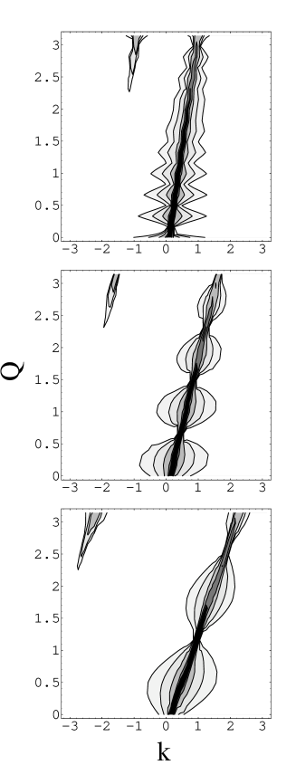
FIG. 2.: The absolute value of $A(Q,k)$ defined in (34) plotted for the filling ratios $c=0.3,0.5$ and 0.7, from top to bottom, respectively. The contours are drawn at 0.03, 0.05, 0.1, 0.3 and 0.5. The appearance of umklapp solution (36) is seen at large $Q$.

FIG. 3.: a) The amplitudes of the solutions $\alpha_{1,2}(Q)$ as determined by fitting the calculated quantity $A(Q,l)$ with the Eq. (37) at $c=0.5$. b) The same functions shown in the extended range of $Q$.

REFERENCES

- [1] S. Tomonaga, Prog. Theor. Phys. (Kyoto), 5, 544, (1950).
- [2] D.C. Mattis, E.H. Lieb, J. Math. Phys. 6 , 304 (1965).
- [3] H. Westfahl Jr., A.H. Castro Neto and A.O. Caldeira, Phys. Rev. B 55, R7347 (1997) and references therein; Dror Orgad, Phys. Rev. Lett. 79, 475 (1997).
- [4] A.E. Sikkema, Ian Affleck ans S.R. White, Phys. Rev. Lett. 79, 929 (1997); Jinwu Ye, ibid., 1385 (1997).
- [5] A.Luther, Phys.Rev. B50, 11446 (1994).
- [6] H.J. Kwon, A. Houghton and B. Marston, Phys. Rev. B 52, 8002 (1995); A.H. Castro Neto and Eduardo Fradkin, Phys. Rev. B 51, 4084 (1995); P. Kopietz and G.E. Castilla, Phys.Rev.Lett. 76, 4777 (1996).
- [7] D.N. Aristov and D. R. Grempel, Phys. Rev. B 55, 11358 (1997).
- [8] D.G. Shelton, A.A.Nersesyan and A.M.Tsvelik, Phys. Rev. B 53, 8521 (1996); E. Orignac and T. Giamarchi, cond-mat 9709297, submitted to Phys.Rev.B.
- [9] J.M. Luttinger, J. Math. Phys. 4 , 1154 (1963).
- [10] E.W. Montroll, R.B. Potts and J.C. Ward, J. Math. Phys. 4 , 308 (1963).
- [11] A. Luther, I. Peshel, Phys.Rev. B 12, 3908 (1975).
- [12] F.D.M. Haldane , J.Phys.C 14, 2585 (1981).
- [13] The proper choice of the cutoff appeared to be most subtle issue for the bosonization approach. See e.g. Ref.[16] ; P.A. Lee, Phys.Rev.Lett. 34, 1247 (1975) ; A. Theumann, Phys.Rev. B 15, 4524 (1977) .
- [14] see for the excellent review : J. Sólyom, Adv. in Physics 28, 201 (1979).
- [15] E. Lieb, T. Schultz, D. Mattis, Ann. of Phys. 16, 407 (1961).
- [16] J.B. Zuber and C. Itzykson, Phys.Rev. D 15, 2875 (1977); see also R. Shankar, Acta Phys. Polonica 26, 1835 (1995).
- [17] see e.g. A.A. Abrikosov, L.P. Gor’kov and I.E. Dzialoshinskii, Quantum Field Theoretical Methods in Statistical Physics (Pergamon Press, New York, 1965).
- [18] The fact of non-zero anticommutator does not change the Eq. (26), though it demands more sophisticated arguments. [17]
- [19] U. Grenander and G. Szego, Toeplitz Forms and their Applications, (University of California Press, Berkeley and Los Angeles, 1958).
- [20] B.M. McCoy and T.T.Wu, Chapter X of The two-dimensional Ising Model, (Harvard University Press, Cambridge Mass, 1973).
- [21] T.T.Wu, B.M. McCoy, C.A. Tracy, E. Barouch, Phys.Rev.B13, 316 (1976); see also V.N. Popov, LOMI proceedings, 77, 188 (Leningrad ,1978), in russian.
- [22] see e.g. I.S. Gradshtein, I.W. Ryzhik, Tables of Integrals, Series and Products, (Academic, New York, 1965).
- [23] H.J. Schulz, Phys.Rev.Lett. 64,2831 (1990); T. Giamarchi and H.J. Schulz, Phys.Rev.B39, 4620 (1989).
- [24] A similar problem was discussed in J. Villain, and P. Bak, J. Physique, 42, 657 (1981).
- [25] For clarity we omit here the coherence factor arising from consideration of half-integer sites. It was shown in [7] that this factor produces some additional modulation of the observable quantity .
- [26] G. Müller, H. Thomas, H. Beck, J.C. Bonner, Phys.Rev. B 24, 1429 (1981).