Interacting electrons with spin in a one–dimensional dirty wire connected to leads

Abstract

We investigate a one–dimensional wire of interacting electrons connected to one–dimensional noninteracting leads in the absence and in the presence of a backscattering potential. The ballistic wire separates the charge and spin parts of an incident electron even in the noninteracting leads. The Fourier transform of nonlocal correlation functions are computed for $T\gg\omega$. In particular, this allows us to study the proximity effect, related to the Andreev reflection. A new type of proximity effect emerges when the wire has normally a tendency towards Wigner crystal formation. The latter is suppressed by the leads below a space–dependent crossover temperature; it gets dominated everywhere by the $2k_{F}$ CDW at $T<L^{\frac{3}{2}(K-1)}$ for short range interactions with parameter $K<1/3$. The lowest–order renormalization equations of a weak backscattering potential are derived explicitly at finite temperature. A perturbative expression for the conductance in the presence of a potential with arbitrary spatial extension is given. It depends on the interactions, but is also affected by the noninteracting leads, especially for very repulsive interactions, $K<1/3$. This leads to various regimes, depending on temperature and on $K$. For randomly distributed weak impurities, we compute the conductance fluctuations, equal to that of ${\mathcal{R}}=g-2e^{2}/h$. While the behavior of $Var({\mathcal{R}})$ depends on the interaction parameters, and is different for electrons with or without spin, and for $K<1/3$ or $K>1/3$, the ratio $Var({\mathcal{R}})/{\mathcal{R}}^{2}$ stays always of the same order: it is equal to $L_{T}/L\ll 1$ in the high temperature limit, then saturates at $1/2$ in the low temperature limit, indicating that the relative fluctuations of ${\mathcal{R}}$ increase as one lowers the temperature.

I Introduction

One–dimensional quantum wires provide an interesting opportunity to study mesoscopic physics in an interacting system. On the one hand, it is well established theoretically that interactions give rise to unique electronic properties in one dimension, described by the so called Tomonaga–Luttinger liquid (TLL) model.[1] A detailed comprehension of the remarkable interplay between interactions and disorder has been achieved.[2, 3, 4, 5] On the other hand, little attention has been paid to the role of the contacts which are known to influence strongly the transport properties of mesoscopic structures and quantum wires. In this respect, two simplified models were proposed recently. Either one connects a finite wire to the reservoirs by tunneling barriers,[6] leading to the suppression of the ballistic conductance at low temperature due to the dramatic effect of the interactions. Alternatively, in the opposite situation, the wire is perfectly connected to one–dimensional leads,[7, 8] yielding a perfect conductance independent on the interactions of any range less than the wire length.[9] The latter result contradicts the conductance reduction by the interactions predicted in a wire without contacts,[4, 5] and is in agreement with recent experiments on micron–length quantum wires.[10, 11] The perfect conductance can be explained through an extension of Landauer’s approach to the interacting wire.[12] The reservoirs are taken into account by the flux they inject which acts as an initial condition for the equation of motion of the density.[7] The incident flux is perfectly transmitted for any range of interactions. But reservoirs inject electrons which are not the proper modes of the wire. This leads us to introduce intermediate noninteracting leads so that we can properly identify the injected and transmitted electronic flux. Under theses circumstances an incident electron undergoes multiple internal reflections at the contacts due to change in interactions, leading to a perfect transmission into a series of spatially separated charges.[7]

While the ballistic conductance of a quantum wire cannot reveal the TLL character of the wire, the natural question one asks is if the other spectacular manifestations of the TLL model, that are the signature of its non–Fermi–liquid behavior, can be still observed. It is the purpose of this paper to study these features. Some have already been addressed in the literature,[13, 14, 15, 16] but new interesting effects of the leads will be seen to appear. We will also discuss recent experiments on quantum wires.[10, 11]

Beyond these points, in the present paper we develop a formal framework to deal with the properties of any inhomogeneous Tomonaga–Luttinger liquid (ITLL). An ITLL can occur in circumstances more general than contact effects. For example, a spatially varying effective interaction can be due to a varying width of the wire or to a nearby gate with a peculiar geometry. One can also think of another ideal system, the edge states in the fractional quantum Hall effect (FQHE).[17] The ITLL model might be relevant to describe transitions between edges at different filling, or an edge state connected to a Fermi liquid.[18, 19, 20] This motivates us to investigate not only electrons with spin but also spinless electrons with external interacting leads.

Let us now summarize our main results. A typical feature of a TLL is the separation of the charge and spin dynamics. Imagine that one injects a spin polarized flux of electrons into one external lead, and detects transmitted spin and charge on the second external lead. Since the latter is noninteracting, one might suspect that charge and spin recombine. But we show that this is not the case: the charge and spin parts are separated even in the noninteracting leads.

Such process has been first studied in refs.[7, 13] for spinless electrons. The propagation is defined in terms of a quasiparticle current (corresponding to Laughlin quasiparticle in the FQHE), and to a superposition of electron-hole excitations in a quantum wire. The basic buildingblock in the description of this effect is the scattering matrix of one quasiparticle at the contact between a TLL of parameter $K_{1}$ and a second one of parameter $K_{2}$.[7, 13, 16] The reflection coefficient is $\gamma=(K_{1}-K_{2})/(K_{1}+K_{2})$, thus is negative when $K_{1}<K_{2}$. Such exotic result indicates an analogy with Andreev[21, 22] reflection even for repulsive interactions.

In connection with this Andreev reflection, we are here led to show a second aspect, the manifestation of proximity effects.[7, 23, 16] It is known that a typical feature of the TLL is the nonuniversal algebraic decay of correlations of different types, reinforcing the tendency towards a CDW or superconducting order which cannot be of long range due to the importance of quantum fluctuations in one dimension. It is important to know the effect of the finite size and of the leads on the fluctuations. We will show here that the dominant tendency in the wire extends towards the external leads.

A new aspect of the “mutual proximity effect” manifests itself when the wire has a tendency towards a Wigner crystal ($4k_{F}$ CDW). This happens usually for Coulomb interactions[24] but also for very repulsive short range interactions. For electrons with spin with charge interaction parameter $K<1/3$, the Wigner crystal dominates the $2k_{F}$ CDW at any temperature in an infinite wire, while the inverse holds at $K>1/3$. With external leads connected to a wire with parameter $K<1/3$, we show the existence of a crossover temperature depending on position $T_{c}(x)$ below which the $2k_{F}$ CDW dominates the Wigner crystal. $T_{c}(x)$ has a non–trivial powerlaw dependence on both the distance to the contacts and the wire length.

The behavior of density correlations can be probed through coupling to a backscattering potential. The effect of weak impurities on the conductance of the wire with leads was found to be qualitatively similar to that without leads,[13, 16, 14, 15] and this seems in agreement with experiments.[10] But compared to the usual TLL, the conductance is affected in a nontrivial way by the contacts, especially when isolated barriers are considered.[13, 15] We show here that for electrons with spin this dependence becomes more crucial for very repulsive interactions because, as mentioned above, the external leads obscure the tendency towards the formation of a Wigner crystal at low temperature.

Apart from the specific model we consider, we improve the study of weak impurities. Usually, the renormalization equations in the presence of one barrier[5] are derived for both the thermal length, $L_{T}\simeq v_{F}/T$, and the wire length, $L$, infinite: their finite values are accounted for semi–empirically by introducing $\inf({L,L_{T}})$ as a cutoff. Here, the renormalization equations are explicitly derived for finite lengths $L$ and $L_{T}$. Besides, they are extended to a backscattering potential whose total spatial extension is less than $L_{T}$ and $L$.

Another important question concerns the fluctuations of the conductance in the presence of a random potential distribution. This question can arise in experiments even if the mean free path is much larger than the wire length due to the imperfection and roughness on the boundaries. Here we show that the conductance is self-averaging at high temperature, more precisely $Var({\mathcal{R}})/{\mathcal{R}}^{2}$ is of the order $L/L_{T}\ll 1$.[25] But this ratio saturates at $1/2$ at temperatures low compared to $T_{L}=u/L$. This has to be taken seriously into account when one tries to infer precise powerlaws from the experimental value of $g$.

Let us now give the plan of our paper which does not follow the above sequence of results. Instead, we separate the paper in two parts: the first deals with spinless electrons which are also relevant for the FQHE, while we restore spin in the second part. For spinless electrons, we begin by describing the formalism and the inhomogeneous Luttinger liquid model. We discuss the discontinuous interaction case which is suitable to understand qualitatively the results; it might be relevant for edge states in FQHE, but is has to be taken with some caution for quantum wires.

We then study the density–density correlation functions for two reasons. First, in order to show how the dominant tendency in the wire extends towards the external leads, in analogy with proximity effects. Next, to investigate the role of backscattering. In particular, the nonlocal correlation functions at finite temperature and at low frequencies are computed. Any extended non–random weak potential is then considered, for which the leading renormalization equation is derived explicitly at finite temperature. The conductance is expressed perturbatively in the backscattering potential. We discuss the random–impurity case where the most important new result concerns the conductance fluctuations.

In the second part dealing with electrons with spin, most of the spinless treatment can be extended except for two important points. First, the transmission process is studied explicitly. Secondly, we show in which way leads affect the tendency towards the Wigner crystal that exists for very repulsive short range interactions. This induces different regimes for the correction to the conductance in the presence of a backscattering potential. Finally, we discuss the experimental results obtained in quantum wires.

II Spinless electrons

A Model

In a strictly one–dimensional system with short range interactions between spinless electrons the low–energy properties can be fully parameterized by two parameters $u$ and $K$. Without interactions $u=v_{F}$ and $K=1$. The Hamiltonian can then be expressed as

$$H=\int\frac{dx}{2\pi}\left[uK\Pi^{2}+\frac{u}{K}(\partial_{x}\Phi)^{2}\right],$$ (1)

where $\Phi$ is related to the long-wavelength component of the electron density through $\rho=-\partial_{x}\Phi/\pi$, and $\Pi$ is the canonical momentum conjugate to $\Phi$, $\left[\Phi(x),\Pi(y)\right]=i\pi\delta(x-y)$. Taking into account the discreteness of the electrons, Haldane derived the representation of the total electron density in terms of $\Phi$:[26]

$$\rho=-\frac{1}{\pi}\partial_{x}\widetilde{\Phi}\sum_{m=-\infty}^{\infty}c_{m}e^{2im\widetilde{\Phi}}.$$ (2)

where $\widetilde{\Phi}(x)=\Phi(x)+k_{F}x$. The coefficients $c_{m}$ obey $c_{-m}=c_{m}$. For the noninteracting case only $c_{0}$ and $c_{\pm 1}$ are nonzero, however in the presence of interactions higher coefficients appear. The $c_{m}$ then can be calculated perturbatively, as done implicitly in ref.[27].

Consider now an interacting wire delimited by $[-a,a]$ whose length will be denoted by

$$L=2a,$$

connected perfectly to non–interacting leads. The global system is described by the Hamiltonian (1) with spatially varying parameters $u(x)$, and $K(x)$.[7, 8] We require $u$ and $K$ to be uniform on the external leads, i.e. for $|x|>L/2$, taking values $u_{L}$ and $K_{L}$. Even though the most relevant situation of noninteracting leads corresponds to $u=v_{F}$ and $K_{L}=1$, it is interesting to keep $K_{L}$ for other possible applications, for instance the FQHE.[19]

We note that the absence of translational invariance in the quantum wire gives rise to an inhomogeneous chemical potential $\mu(x)$ that can be incorporated by a translation in $\Phi$.[16] Then one has to replace, in eq.(2),

$$-k_{F}x\rightarrow\phi_{0}(x)=-k_{F}x+\int^{x}dx^{\prime}\,\mu\frac{K}{u}.$$ (3)

Let us discuss the microscopic arguments for the ITLL model. If one assumes that the screening does not take place in the same way in the two–dimensional gas into which the wire opens and inside the wire we can argue that interactions are described by a function $U(x,y)$ which is not translationally invariant. But then the electronic momentum is not conserved anymore in the vicinity of the contacts. Indeed, this appears when one bosonizes the interaction Hamiltonian $\int\int U(x,y)\rho(x)\rho(y)$, using $\rho$ from eq.(2): the exponential terms in $\Phi$ cannot be ignored in general, and those terms violate momentum conservation. But if $U(x,y)=f(x)f(y)h(x-y)$ where $f$ varies slowly on scales $\lambda_{F}$, one can reduce the Hamiltonian to a quadratic form.[16, 12] Strictly speaking, this condition is required to find a perfect conductance, as discussed in ref.[12]. If this condition is not met, and for not too strong interactions, the perfect conductance is recovered in the high temperature limit, but is reduced due to the abrupt change in interactions at low temperature. For instance, when $u(x)=u$ and $K(x)=K$ are constants for $|x|<L/2$, exponential terms in $\Phi(\pm a)$ cannot be ignored, and give rise to effective barriers determined by the jump of the interactions. Nevertheless, due to the symmetry of the structure, and since one needs $k_{F}L\gg 1$ to be able to use the TLL model, one can easily achieve resonances that suppress the role of these terms.

For quantum wires opening adiabatically into a two–dimensional gas, the situation of abrupt variations is not realistic; it is adopted for mathematical convenience, and the results can be be trusted only far from the contacts compared to $\lambda_{F}$ where the behavior should not depend on the profile of variations at the contacts. We shall however look at the behavior at the contact because it is very similar to that in the strong tunneling limit of two coupled Luttinger liquids:[20] the effective parameter at the contact, yielding the local conductance [7] and controlling the correlation functions[13] is exactly the same as the parameter for the equivalent TLL liquid in ref.[20].

The situation for edge states in the fractional quantum Hall effect (FQHE) might be different. Non–quadratic terms arise from tunneling between edge states, which is more difficult to achieve due to their spatial separation. Recently, the model with discontinuous parameters was shown to be suited to describe transitions between edges with different filling,[19] or the connection between an edge state and a Fermi liquid.[20] In any case, most of the results we derive here can be extended to any profile of variations of the parameters.

B Correlation functions

It is well known that symmetry breaking phase transitions cannot occur in one dimension. But the interactions in an infinite wire enhance charge density or superconducting fluctuations depending on whether they are repulsive or attractive. The natural question is to know whether such tendencies persist in the presence of leads.

In the present subsection, we would like to compute the correlation functions not only to answer this question, but also to explain the proximity effect,[7, 23, 16] and to give the necessary tools for studying the role of backscattering in the next section, closely related to the tendency towards formation of a charge density wave.

1 Correlation functions at finite temperature

Let us write the density–density correlation function, using eq.(2):

$$\left\langle T_{\tau}\rho(x,\tau)\rho(y,0)\right\rangle=-\partial_{x}\partial_{y}\left[U(x,y,\tau)+\phantom{\sum_{m\neq 0}}\right.$$ (5)

$$\left.\sum_{m\neq 0}\frac{c_{m}^{2}}{2m^{2}}X_{m}(x,y,\tau)e^{2im[\phi_{0}(x)-\phi_{0}(y)]}\right],$$

where $U$ is given in terms of the fundamental bosonic Green function[28]

$$G(x,y,\tau)=\left\langle T_{\tau}\Phi(x,\tau)\Phi(y,0)\right\rangle,$$ (6)

as

$$U(x,y,\tau)=G(x,x,\tau_{0})+G(y,y,\tau_{0})-2G(x,y,\tau).$$ (7)

$\tau_{0}$ is a cutoff different but in general of the order of $1/E_{F}$. We impose on the imaginary time $\tau>\tau_{0}$, so that $G$ can be computed at finite temperature, without dependence on $\tau_{0}$.[16]The consequence of this cutoff procedure on analytic continuation is elucidated in appendix B.

In eq.(5) $\phi_{0}$ is given by eq.(3), and

$$X_{m}(x,y,\tau) = \left\langle T_{\tau}e^{im\Phi(x,\tau)}e^{-im\Phi(y,0)}\right\rangle$$ (9)

$$=e^{-2m^{2}U(x,y,\tau)}.$$

Note that the first term (in $U$) in eq.(5) can be obtained from the limit $m\rightarrow 0$ of $X_{m}$.

Instead of writing out explicitly $X_{m}$ the imaginary part of its Fourier transform in the low frequency limit $\omega\ll T$ will be of more use:

$${\mathcal{I}}mX_{m}(x,y,\omega\ll T)\sim-\frac{\omega}{E_{F}^{2}}\chi_{m}(x,y),$$ (10)

where $\chi_{m}(x,y)$ is a dimensionless function. The function $\chi_{m}$ can be obtained from $\chi_{1}$ by multiplying $K(x)$ by $m^{2}$, thus we will often study $\chi_{1}$, denoted $\chi$ for simplicity. The time dependence of $U$ being due to the nonlocal part $G(x,y,\tau)$ in eq.(7), we can write (for details see appendix B)

$$\chi\left(x,y\right)=\frac{1}{\underline{T}^{2}}C(x,y)e^{-2G(x,x,\tau_{0})}e^{-2G(y,y,\tau_{0})},$$ (11)

where

$$\underline{T}=T\tau_{0}$$ (12)

and $C$ is a dimensionless time integral, eq.(B14). We can find the properties of $C(x,y)$ for general smooth variations of $K$ and $u$, and we have computed it explicitly for any $x,y$ in the discontinuous interaction case and at finite temperature. By deforming the contour of integration in the complex plane, the computation is made much easier, especially in the low temperature limit. In the high temperature limit, more steps are needed. The results are given explicitly in appendix B.

In an infinite wire with uniform parameter $K$, $\chi(x,y)$ is a function of $x-y$, and we denote it by $\chi^{(K)}(x-y)$. It decreases exponentially at separations larger than $L_{T}=\pi u/T$, $\chi^{(K)}(r)=(r/L_{T})e^{-Kr/L_{T}}$, while its local value has the typical powerlaw in temperature $\chi^{(K)}(r=0)\simeq T^{2(K-1)}$ that diverges in the zero temperature limit when $K<1$, indicating an enhancement of the density fluctuations compared to the noninteracting case.

For interaction parameters $u,K$ constant in the bulk of the wire and reaching their asymptotic values $u_{L},K_{L}$ on the external leads, four general properties of $\chi$ can be shown. The first and second one hold at high temperature, where comparison can be made with $\chi^{(K)}$.

1. At $T\gg T_{L}$, we have

   $$a-|x|,a-|y|\gg L_{T}\Rightarrow\chi(x,y)\simeq\chi^{(K)}(x-y)$$ (13)

   where $\chi^{(K)}(x-y)$ is the value of $\chi$ in an infinite wire with parameter $K$. Thus we recover the translationally invariant behavior for any $x,y$ far from the contacts compared to $L_{T}$.

2. Again, at $T\gg T_{L}$, but for any location of $x,y$, we have

   $$\chi(x,y)\leq\chi^{(K)}(x-y)$$ (14)

   for $K_{L}>K$, while the inverse inequality holds for $K_{L}<K$.

3. At any temperature, and for small separations compared to $L_{T}$, $\chi$ factorizes:

   $$\left|x-y\right|\ll L_{T}\Longrightarrow\chi(x,y)\simeq\sqrt{\chi(x,x)}\sqrt{\chi(y,y)}.$$ (15)

   This is due to the fact that $C(x,y)\sim C(x,x)$ [eq.(11)], up to corrections of order $(|x-y|/L_{T})^{2}$.

4. The local value of $\chi$ is almost constant on segments much less than the wire length and the thermal length. If we denote

   $$L_{min}=\min(L,L_{T}),$$ (16)

   then

   $$\left|x-y\right|\ll L_{min}\Longrightarrow\chi(x,x)\simeq\chi(y,y)\sim\chi(x,y).$$ (17)

   These equalities hold up to corrections of the order of $(|x-y|/L_{min})^{2}$.

Let us now specialize to the case of discontinuous parameters. First we introduce the quasiparticle density $j_{r}=j+ru\rho$ for $r=\pm$ which are the right– and left–going proper modes in a uniform TLL. They correspond to Laughlin quasiparticle currents in edge states of the FQHE. As we said before, the basic quantity for understanding the physics is the scattering matrix[7, 13, 16] of quasiparticles at the contact of two perfectly connected TLL with parameters $K$ and $K_{L}$. It acts in the space $(j_{+},j_{-})$ and is given by

$$S=\left(\begin{array}[]{cc}-\gamma&1+\gamma\\ 1-\gamma&\gamma\end{array}\right)$$ (18)

where $\gamma$ is the reflection coefficient

$$\gamma=\frac{K_{L}-K}{K_{L}+K}.$$ (19)

The matrix $S$ relates the outgoing flux to the injected flux, defined not in term of wavefunction amplitudes as in usual scattering approaches, but directly in terms of the quasiparticle current $j_{r}$. The local effective parameter (yielding a local Kubo conductance[7, 16]) is given by $K_{1}$ multiplied by the transmission coefficient,[7, 23]

$$K_{a}=K_{L}(1-\gamma)=K(1+\gamma).$$ (20)

Let us first discuss the high temperature limit. It is worth noting that a lower (upper) bound to $\chi(x,y)$, completing eq.(14), is given by $\chi^{(K_{a})}(x-y)$ for $K_{L}\geq K$ ($K_{L}\leq K$). In eq.(11), the nonlocal part $C(x,y)$ is given by eq.(LABEL:CF1) in the limit $T\gg T_{L}$, while it simplifies to a constant [eq.(B32)] in the limit $T\ll T_{L}$, in accordance with property (15). The Green function $G$ is given by eq.(B16). Instead of writing explicitly the factor $e^{-2G(x,x,\tau_{0})}$ that enters in eq.(11), we use the local value of $\chi$. This is equivalent as far as the dominant behavior is concerned because $C(x,x)$ is a slowly varying function of $x$ (cf. appendix B). Thus we drop it from

$$\sqrt{\chi(x,x)}\simeq\frac{1}{\underline{T}}e^{-2G(x,x,\tau_{0})}.$$ (21)

In the high temperature limit $(T>T_{L}$), the multiple reflections caused by the change in interactions don’t affect the correlation functions due to the lack of thermal coherence along the wire. Only one reflection is felt within a thermal length $L_{T}=u/T$ from the contacts. We now define

$$t_{x}=\frac{a-|x|}{u\tau_{0}},$$ (22)

the time it takes for a quasiparticle emanating at $x$ to reach the closest contact, measured in units of $\tau_{0}$. For $t_{x}\gg 1$ [eq.(22)], we find

$$\sqrt{\chi(x,x)} \sim \underline{T}^{K-1}(\tanh{}\underline{T}t_{x})^{K_{a}-K}.$$ (23)

Again, for points far from the contacts compared to $L_{T}$, this expression coincides with that obtained in an infinite TLL with parameter $K$, $\chi\sim\underline{T}^{2(K-1)}$. At the contacts, we find $\chi(a,a)\simeq\sim\underline{T}^{2(K_{a}-1)}$ [cf eq.(B29)] (this amounts to setting $t_{x}=1$ in eq.(23), using $\underline{T}\ll 1$).

In the limit of temperatures low compared to $T_{L}$, the multiple reflections affect the correlation functions, thus the external leads with parameter $K_{L}$ determine the temperature dependence. But there is a nontrivial dependence on the wire length as well as on the distance of the barrier from the contacts:

$$\sqrt{\chi(x,x)}\simeq \underline{T}^{K_{L}-1}\underline{T}_{L}^{K_{a}-K_{L}}t_{x}^{K_{a}-K}.$$ (24)

This gives the behavior for $t_{x}\gg 1$. $\chi(a,a)$ can be obtained by setting $t_{x}=1$ in this expression.

Remember that one obtains $\chi_{m}(x,x)$ from $\chi(x,x)$ (in both temperature limits) by multiplying both $K$ and $K_{L}$ by $m^{2}$, which leaves $\gamma$ [eq.(19)] unchanged. Clearly, the $2mk_{F}$ CDW is less important than the $2k_{F}$ one. Further, if electrons in the external leads are non interacting, $K_{L}=1$, the $2mk_{F}$ CDW are suppressed in the zero-temperature limit because $\chi_{m}\sim T^{2(m^{2}K_{L}-1)}=T^{2(m^{2}-1)}$ [eq.(24)].

2 Proximity effect

Let us first recall an exotic phenomena emanating from this model, the analogy with Andreev reflection.[7, 23, 16]

a Andreev reflection

The reflection coefficient of a quasiparticle from a TLL with parameter $K_{1}$ incident on another one with parameter $K_{2}$ is given by $\gamma$, eq.(19), and is negative for $K_{1}<K_{2}$, i.e. a partial quasi-hole is reflected back. This is similar to Andreev reflection of an incident electron on a normal–superconductor interface. The similarity is the closest for $K_{1}=1$ and $K_{2}>1$, because the wire has a tendency towards superconductivity, but it holds more generally even for repulsive interactions, for instance for a quasiparticle in the wire with $K<1$ incident on the noninteracting lead.

It is worth noting that in the case of two semi–infinite wires with $K_{1}$ and $K_{2}$ as parameters, and $K_{1}<K_{2}$, the local Kubo conductance at the interface is given by the transmission coefficient from $1$ to $2$ multiplied by $K_{1}$, i.e. by $g_{a}=K_{a}$. This verifies $K_{1}\leq g_{a}\leq 2K_{1}$.[7, 23, 16] This is very similar to the inequalities for an N-S interface, if one interprets $K_{1}$ as the conductance (Kubo) of the normal side, $g_{N}\leq g_{N-S}\leq 2g_{N}$.[29]

Finally, let us comment on a recent paper[30] based on the model in ref.[20] of two TLLs connected by a tunneling term. The bosonized theory was associated with conformal field theories to describe quasiparticles in term of soliton states. Interestingly, in the strong tunneling limit, the scattering matrix for these states at the interface turns out to be the same as eq.(18). This gives a stronger foundation of the quasiparticle scattering scheme we introduced previously.[7]

b Proximity effect

The reflection at the contact gives rise to a proximity effect for both superconducting or CDW correlations.[7, 23, 16, 31] This can be seen computing the correlation functions on the external leads. In particular, when $T\gg T_{L}$, there is no coherence between the endpoints of the wire, and it is sufficient to consider half the system. The wire and one lead have a symmetric role; it is sufficient to permute $K$ and $K_{L}$ in eq.(23) in order to find $\chi$ for $|x|>a$, and to take $t_{x}=(|x|-a)/u_{L}$. By the way, this situation is relevant for the FQHE, if two edge states with different filling are connected.[19]

At $T<T_{L}$, instead of eq.(24) inside the wire, outside the wire one has

$$\sqrt{\chi(x,x)}\simeq\underline{T}^{K_{L}-1}(\underline{T}_{L}t_{x})^{K_{a}-K_{L}}$$

up to $t_{x}T_{L}\sim 1$. Beyond a distance of the order of $L$ in one external lead, we recover the simple law $T^{K_{L}-1}$.

For clarity, we discuss the consequence for noninteracting leads, $K_{L}=1$. Then if $K<1$, the density–density correlations in the bulk are similar to those in an infinite wire, but are reduced when one goes to the contacts because $t_{x}^{\gamma K}$ decreases for $\gamma>0$. Besides, this enhancement extends in the external leads up to a distance $L_{min}/K$ [eq.(16)].[23, 16] For $K>1$, the pairing correlation function, which can be obtained from $\chi$ if one replaces $K$ by $1/K$ and $K_{L}$ by $1/K_{L}$, is enhanced up to a distance $KL_{min}$. This increases with $K$, i.e. where interactions are more attractive. This is reminiscent of the proximity effect.[29]

In general, we can show that the proximity effect extends up to the minimum length scale at hand. We must note that this holds even for a smooth profile of $u$ and $K$, as for instance the properties of $\chi$ exposed before are general.

C Backscattering by non–random impurities

We study now the role of impurities in the wire. The conductance with impurities was shown to depend on the interactions and is generally affected by the external leads.[13, 14, 15, 16, 23] The main goal of this part is to give a general scheme to treat the effect of a weak backscattering potential $V(x)$ in a non–translational invariant system and at finite temperature.

1 Renormalization Equations

The coupling of the conduction electrons to impurities with potential $V(x)$ is $\int dxV(x)\rho(x)$, where $\rho$ is given by eq.(2). It is then convenient to do an integration by parts giving [32]

$$H_{imp}=\int\rho(x)V(x)=\sum_{m=-\infty,m\neq 0}^{\infty}\int dx\frac{c_{m}V^{\prime}(x)}{2i\pi m}e^{2im\widetilde{\Phi}(x)}.$$ (25)

The forward scattering term $-\partial_{x}\Phi V(x)$ is absorbed by a translation of $\Phi$ by

$$\int^{x}dx^{\prime}\frac{K}{u}V(x^{\prime})$$ (26)

which has to be included in the scalar function $\phi_{0}$, eq.(3).

Note that the impurity Hamiltonian (25) is similar to that considered usually if we replace our $V^{\prime}(x)$ by $-2imV(x)/(c_{m}u\tau_{0})$. For instance, if $V$ has the form of a kink, it corresponds to what is commonly treated as one barrier.

In order to derive the renormalization equations, the exact partition function $Z$ at finite temperature is expanded in terms of $V^{\prime}$:

$$Z = \sum_{n}\frac{(-1)^{n}}{n!}\int\ldots\int\sum_{\sum_{j}m_{j}=0}\prod_{j=1}^{n}c_{m_{j}}V^{\prime}\left(x_{j}\right)e^{2im_{j}\phi_{0}\left(x_{j}\right)}\exp\left(\sum_{i\neq j}m_{i}m_{j}U_{ij}\right),$$ (27)

where $U_{ij}=U\left(x_{i},x_{j},\tau_{i}-\tau_{j}\right)$ is given by eqs.(6,7), and the integration runs over $x_{i}$ and $\tau_{i}$. $Z$ describes a neutral gas of integer charges restricted to a cylinder whose perimeter is $\beta$, and whose height is determined by the spatial extension of $V^{\prime}$, reducing to a circle when $V^{\prime}$ is local. The charges interact via $U(x,y,\tau)$, eq.(7). This is not the Coulomb interaction but an infinite series of logarithmic terms related to the transmission process discussed earlier (see eq.(B16)).[16] The renormalization procedure is implemented by increasing the cutoff to $\tau_{0}(l)=\tau_{0}e^{l}$, where $\tau_{0}$ is the bare cutoff $1/\Lambda$, and modifying the parameters in order to keep $Z$ invariant. It is immediate to derive the leading–order equation for $V$. According to eq.(7), the cutoff appears in the local part of $U$. The change of $U(x,y,\tau)$ due to a change of the cutoff by $d\tau_{0}$ is

$$\left[\frac{dG}{d\tau}(x,x,\tau_{0}(l))+\frac{dG}{d\tau}(y,y,\tau_{0}(l))\right]d\tau_{0}(l),$$

The exponential of such a term for a pair $x_{i},x_{j}$ factorizes and, once the global neutrality is used, can be absorbed separately into $V^{\prime}(x_{i})$ and $V^{\prime}(x_{j})$. This gives the leading-order flow equations for $V(x)$ explicitly at finite temperature

$$\frac{dV^{\prime}_{m}\left(x,l\right)}{dl}=V^{\prime}_{m}\left(x,l\right)\left(1+2m^{2}\frac{dG}{dl}(x,x,\tau_{0}e^{l})\right).$$ (28)

Note that in the limit of zero temperature, an infinite uniform wire with parameter $K$, and a purely local $V$, the Fourier transform of this equation yields the well-known flow equation for $V(2mk_{F})=V_{m}$, $dV_{m}/dl=V_{m}(1-m^{2}K)$,[5] provided $k_{F}$ is independent on the cutoff as we required.

In general, one expects $V(x)$ to renormalize the interactions. In the extreme case of a local barrier, it was shown by integrating out degrees of freedom away from the barrier that the interactions are not renormalized.[5] We can both recover and generalize this result in a different way, by using the expansion above at finite temperature and in the finite wire: new interaction terms $W$ between the charges are generated by the renormalization, but they decay faster than $U$ at long time scales. For instance, in the zero-temperature limit, and for a barrier in the center of the wire, $U=K\log\tau$ is corrected by $W(\tau,T=0)=K^{\prime}(\log\tau)/\tau$, where $K^{\prime}$ is renormalized by $V$. At finite temperature, we have $W(\tau,T)\leq W(\tau,0)$, i.e. $W$ is still decaying faster than $U$.[16]

Let us now discuss a more extended potential than one barrier, but whose total extension obeys $d\ll L_{min}$ [eq.(16)]. It turns out that when one goes to a cutoff such that $u\tau_{0}(l)>d$, the partition function (27) becomes identical to that of a local barrier.[16] This is related to the property (17). Then it is tempting to assume that the effect of such a potential would be similar to that of a local barrier at length scales larger than the potential extension $d$. But one has to check that the renormalization from the bare cutoff up to $d$ does not modify the local interaction parameter, i.e. $K(x)$ at points where $V^{\prime}(x)\neq 0$. This would induce non translational invariant effective interactions even if the bare $K$ is uniform. We can for instance show that $\phi_{0}$ [eq.(3)] is renormalized by a complicated complex function, whose equation is rather lengthy to write. Thus we think this point needs a more thorough study.

Finally, it is worth writing the next–order corrections to eq.(28) in the case where the partition function becomes equivalent to that of a barrier and therefore the integrations over $x_{i}$ can be done explicitly in eq.(27). For given $m$, one has to add to this equation

$$\sum_{m_{1}+m_{2}=m}V_{m_{1}}V_{m_{2}}$$ (29)

up to nonuniversal prefactors depending on $m_{1},m_{2}$.[16]

If we ignore renormalizations of the interaction, as is surely correct for a local barrier or for a weak enough extended potential, the equation (60) can be integrated straightforwardly. In the absence of an external energy scale, the unique limitation on increasing the cutoff comes naturally from the fact that one has to put at least two charges on the same cylinder of radius $\beta$, thus we stop at $\tau=\beta/2$. Then the renormalized potential is simply

$$V^{\prime}(x,\beta/2)=\sqrt{\chi(x,x)}V^{\prime}(x)$$ (30)

where $\chi(x,x)$, eq.(21), has been studied in the previous subsection.

One can also consider the Fourier transform $V(k)$ of the potential. If the extension of $V$ is less than $L_{\min}$, we can use eq.(17) to factor out $\chi$ from the integral, thus allowing us to recover the dominant term of the renormalized Fourier component of $V$:

$$V_{m}=\int dxV^{\prime}(x)e^{2im\phi_{0}(x)},$$ (31)

by simple multiplication by $\sqrt{\chi_{m}(x,x)}$. Note that whenever $\phi_{0}$ [eq.(3)] can be replaced by $k_{F}x$, $V_{m}=-2imk_{F}V(2mk_{F})$. However the nonlocality of $\chi_{m}$ has to be taken into account when one looks to the next leading term.[32]

The derivation above is valid for any profile of parameters. In case $K$ varies from its external value $K_{L}$ towards a plateaus at $K$ inside the wire, we can show that the dependence of $\chi(x,x)$ on $T$ is monotonic. Its monotony is determined for any $x$ by the sign of $1-K$ at $T>T_{L}$, thus is similar to that in an infinite wire. The renormalized $V^{\prime}$, Eq.(30) obtained at a given temperature goes up (down) when temperature is lowered for $K<1$ ($K>1$). At $T<T_{L}$, the $T$ dependence is controlled by the sign of $1-K_{L}$, in particular $V^{\prime}$ saturates for $K_{L}=1$ at $T<T_{L}$.

In the case of discontinuous parameters, the explicit value of $\chi$ is given by eqs.(23) and (24) for the high and low temperature regime. The renormalized $V$, depending on the location of the barriers, is shown in fig.1 for the case $K_{L}=1$, $K<1$. We point out that these curves are not inferred from cutting the scaling at $T$ or at $T_{L}$, but result from the renormalization at finite temperature and for the finite wire. Note that the saturation at $T<T_{L}$ occurs only for $K_{L}=1$ and for $m=1$.[13, 14]

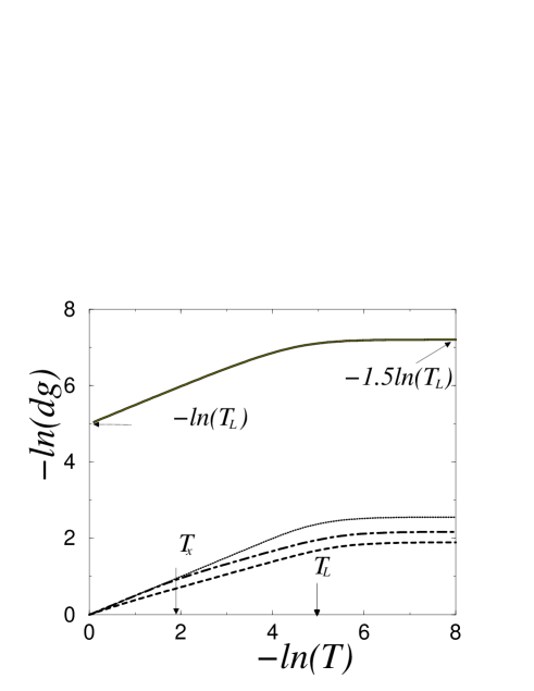
FIG. 1.: The three lower curves show the renormalized barrier strength, whose square yields the dimensionless reduction to the conductance $\mathcal{R}$, scaled by its bare value. The dotted, dashed and dot–dashed curves correspond respectively to a barrier at the center of the wire, at the contact and at an intermediate point $x$. $T$ is in units of $1/\tau_{0}$. We chose $\tau_{0}=T_{L}/148$, thus $-\ln(T_{L}\tau_{0})=5$, and $K_{\rho}=0.5$, $K_{\sigma}=1$. The same curves hold for spinless electrons if one replaces $K_{\rho}$ by $K$, but one has to multiply the $log\mathcal{R}$ by $2$. There is a crossover at $T_{L}$ from a powerlaw controlled by $K_{\rho}$ ($K_{a\rho}=2K_{\rho}/(1+K_{\rho})$) at the center (at the contact) to a plateau. For a barrier at $x$, there are two crossovers, one at $T_{x}=u_{\rho}/t_{x}$ from $T^{K_{\rho}-1}$ to $T^{K_{a\rho}-1}$, followed by a saturation occurring at $T_{L}$. The continuous upper curve corresponds to $l_{e}\left\langle\mathcal{R}\right\rangle/(u\tau_{0})$ for an extended Gaussian distribution, where the powerlaw at $T<T_{L}$ is governed by $K_{\rho}$ since the interactions are repulsive. The $2k_{F}$ backscattering dominates the $4k_{F}$ one for any $T$ since $K_{\rho}=0.5>1/3$.

2 Conductance with non–random impurities

Let us first recall that the conductance of a wire without impurities $g=e^{2}/h$ is independent of interactions if the external leads are noninteracting. The conductance can be related to the transmission, which turns out to be perfect, thus generalizing Landauer’s approach to an interacting wire.[7, 12] One can also use the Kubo formula,[8] provided the external leads are noninteracting, and one is limited to the linear and stationary regime. We have to stress an important point: the external field has to be used when interactions are included exactly in the Hamiltonian, and not the internal electric field modified by the interactions. This is clear for instance through the equation of motion method we have developed in ref.[7] to study transport, for which the external field forms a source term.

The same conditions to justify the Kubo formula hold with impurities, if one assumes that the reservoirs impose an external bias $\Delta V$ (that can be maintained in the noninteracting leads) independently of the current. Then the stationary current is given by

$$j(x) = \lim_{\omega\rightarrow 0}\int\sigma(x,y,\omega)E(y,\omega)$$ (33)

$$=\sigma(x,y)\Delta V$$

where $\sigma(x,y,\omega)$ is the nonlocal conductivity, related to the Fourier transform of $G$ [eq.(6)] computed now with the total Hamiltonian $H+H_{imp}$, and continued to real frequency,

$$\sigma(x,y,\omega)=-\frac{2i\omega}{\pi}G(x,y,\omega).$$ (34)

The uniformity of the current as well as time reversal symmetry require the zero frequency limit of $\sigma(x,y,\omega)$ to be uniform.[33, 7, 16] Thus

$$g=\frac{e^{2}}{h}\sigma(x,y).$$ (35)

.

If the external leads are interacting, one cannot impose an external value of the potential, rather the potential is now renormalized by the interactions.[9, 12] Nevertheless, the spatial separation of the two edges in a Hall bar can lead to different couplings with reservoirs as discussed in [34, 20], and it is also possible to measure locally the potential on each edge. Thus it is still of interest to let the external parameter $K_{L}$ arbitrary.

In appendix A, we derive a novel exact Dyson equation for the conductivity in a non–translationally–invariant system. This is very suitable to write the perturbative expression for the conductance[16]

$$g_{imp}=\frac{e^{2}}{h}\left(1-\mathcal{R}\right),$$ (36)

where $\mathcal{R}$ is given by

$${\mathcal{R}}=\frac{K_{L}}{2\pi}\sum_{m=1}^{\infty}c_{m}^{2}{\mathcal{R}}_{m},$$ (37)

and ${\mathcal{R}}_{m}$ is the contribution from backscattering of $m$ electrons,

$${\mathcal{R}}_{m} = \int\-\-\-\int\chi_{m}(x,y)\frac{V^{\prime}(x)V^{\prime}(y)}{(uk_{F})^{2}}\cos 2m\left[\phi_{0}(x)-\phi_{0}(y)\right],$$ (38)

where $\chi_{m}$ is defined by Eqs. (7,6,10,9). Remember that the forward scattering contribution is included in $\phi_{0}$ [eq.(26)]. We have already obtained general properties of $\chi(x,y)$. If parameters change abruptly, one can inject the explicit form (appendix B) to express the conductance at any temperature, for sufficient weak potential with any extension.

If the potential extension is much less than $L_{min}$ [eq.(16)], we can use eq.(17) to show easily that the dominant term of equation (38) reduces to the square of the renormalized potential

$${\mathcal{R}}_{m}\simeq\chi_{m}(x,x)|V_{m}|^{2}$$ (39)

where $V_{m}$ is given by eq.(31). As long as $V_{1}\neq 0$ (i.e. out of resonance), the dominant term in $\mathcal{R}$ is given by ${\mathcal{R}}_{1}$. On resonance, the dominant term comes still from $m=1$ or from $m=2$;[32] this depends on the values of $K$ and $K_{L}$, as well as the extension and strength of the potential. It appears that at low temperature, because the $4k_{F}$ CDW correlation function acquires a factor $T^{2(4K_{L}-1)}$ [eq.(24) with $K$ and $K_{L}$ multiplied by $4$], one must have $K_{L}>1/4$ for $\mathcal{R}$ to vanish at zero temperature (for a short enough wire). Remarkably, for $K_{L}=1$, the low temperature conductance is still $e^{2}/h$ on resonance, even for $K<1/4$. We will not discuss the resonance in further detail here, even though one has a variety of behaviors, and we refer to the explicit expression of $\mathcal{R}$, Eqs.(3738), and to the computation of appendix B.

Out of resonance, and for discontinuous parameters, $K_{L}=1$, $\mathcal{R}$ is given by the same curves as those yielding the renormalized $V$ in fig.1. The wire has to be short enough so that $\mathcal{R}$ stays weak enough when reaching the plateaus below $T_{L}$, otherwise the perturbative computation breaks down at a temperature above $T_{L}$. We refer to ref.[15] for the strong barrier case.

D Random impurities: conductance fluctuations

Now we consider random impurities distributed all over the wire. For simplicity, we limit ourselves to the case of a Gaussian distribution, $\left\langle V(x)\right\rangle=0$, and

$$\left\langle V(x)V(y)\right\rangle=D\delta(x-y).$$ (40)

By averaging eq.(38) over disorder, one obtains the leading term of $\mathcal{R}$ [eq.(37)] coming from the $m=1$ contribution

$$\left\langle\mathcal{R}\right\rangle=K_{L}\int_{-a}^{a}\frac{dx}{l_{e}(x)}\chi(x,x),$$ (41)

where $1/l_{e}(x)=4D[\phi_{0}^{\prime}(x)]^{2}/(uk_{F})^{2}$. The forward scattering part in $\phi_{0}^{\prime}$ is $KV(x)/u$ [eq.(26)], and thus can be dropped when averaging. Thus the dependence of $l_{e}$ on $x$ is due to the inhomogeneity of the interactions. It could also be induced by a space–dependent disorder strength $D(x)$. Nevertheless, we will assume $\phi_{0}^{\prime}(x)\simeq k_{F}$ for simplicity, in which case $l_{e}$ is uniform and is equal to $D/u^{2}$. This holds for instance in the bulk of the wire, and thus this is a plausible approximation whenever the impurities in the bulk dominate.

Note that we have obtained eq.(41) by performing first a double integration by parts in eq.(38) and then retaining only the term with no derivative of $\chi$. The explicit integration of the function $\chi$ can be done but is tedious. However, the results can be understood easily.[13, 16] There are two main contributions: one from the bulk that behaves, for $T>T_{L}$, as $LT^{2(K-1)}$, the other from the contacts behaving as $T^{2(K_{a}-1)}$. For $T<T_{L}$, up to nonuniversal constants, these contributions become[13, 16]

$$\left\langle{\mathcal{R}}\right\rangle\simeq\frac{u\tau_{0}}{l_{e}}\underline{T}^{2(K_{L}-1)}\left[T_{L}^{2(K-K_{L})-1}+T_{L}^{2(K_{a}-K_{L})}\right]$$ (42)

where $K_{a}$ is given by eq.(20).

Let us discuss the case of noninteracting leads, $K_{L}=1$. In this case, the contact contribution dominates for very attractive interactions, $K>(3+\sqrt{1}7)/2$, and for not too high temperatures (or not too long wires).

Inspecting eq.(42), we see that $\left\langle{\mathcal{R}}\right\rangle$ saturates at $T<T_{L}$ at a value $\ll 1$ for $K>3/2$, but that it increases with wire length for $K<3/2$. In the latter case, the perturbative computation is valid only for $L<L_{loc}$ where

$$L_{loc}\sim u\tau_{0}\left(\frac{l_{e}}{u\tau_{0}}\right)^{\frac{1}{3-2K}}.$$ (43)

This coincides with the localization length inferred by scaling arguments in [4, 3].

Let us now compute the variance of the conductance $Var(g)=\left\langle g^{2}\right\rangle-\left\langle g\right\rangle^{2}$. Clearly, it is also equal to the variance of $\mathcal{R}$ which can be expressed perturbatively, using eq.(38), as

$$Var({\mathcal{R}})=K_{L}^{2}\int_{-a}^{a}\int_{-a}^{a}\frac{dxdy}{l_{e}^{2}}\cos^{2}2\left[\phi_{0}(x)-\phi_{0}(y)\right]\chi^{2}(x,y).$$ (44)

Here we have used eq.(40) to perform the average of ${\mathcal{R}}^{2}$, have dropped the product of two correlation functions for different pairs of integers, and neglected the role of the derivative in eq.(25).

It is interesting to consider first the low temperature limit $T<T_{L}$, where a general inequality, valid for arbitrary profile $K(x)$, can be shown. Using the factorization property (15) which holds now for any $x,y$ in the wire because $L\ll L_{T}$, we can write eq.(44) as

$$Var({\mathcal{R}})=\sum_{r=\pm 1}\frac{K_{L}^{2}}{2}\left|\int_{-a}^{a}\frac{dx}{l_{e}}e^{2i(1+r)\phi_{0}(x)}\chi(x,x)\right|^{2}.$$ (45)

The term for $r=1$ on the right hand side is less than that for $r=-1$, this latter is nothing but $\left\langle{\mathcal{R}}\right\rangle^{2}$ [eq.(41)]. Thus we have the interesting inequality

$$\frac{1}{2}\left\langle\mathcal{R}\right\rangle^{2}\leq Var({\mathcal{R}})\leq\left\langle\mathcal{R}\right\rangle^{2}.$$ (46)

In particular, this shows that

$$\frac{Var({\mathcal{R}})}{\left\langle\mathcal{R}\right\rangle^{2}}\simeq\frac{1}{2}.$$ (47)

If $\phi_{0}(x)$ is simply $k_{F}x$, this is a very good estimate of $Var({\mathcal{R}})$ because the integral for $r=1$ in eq.(45) contains a rapidly oscillating function, $e^{2ik_{F}x}$, while $\chi$ varies slowly compared to $\pi/k_{F}$. Besides, $Lk_{F}\gg 1$ in order to validate the bosonization, so that the integral corresponding to $r=1$ in eq.(45) can be neglected. This justifies eq.(47), showing that the fluctuations of $\mathcal{R}$ are of the same order as its average value. In the special case of short range interactions with discontinuous parameters, $Var({\mathcal{R}})$ is obtained as the square of eq.(42).

We now consider the high temperature limit, $T>T_{L}$. To simplify the discussion, we restrict ourselves to the case $K<1$, which is probably the case in a quantum wire. Then the bulk contribution dominates over the contact effects, so that we can restrict the integral in eq.(44) to $-a/2,a/2$, and therefore $t_{x}T\gg 1$. Over this segment, $\chi$ depends only on $x-y$ ( see eq.(13)), and we can write, after a change of variables $x-y=vL_{T}$,

$$Var({\mathcal{R}})\simeq\frac{LL_{T}}{l_{e}^{2}}\underline{T}^{4(K-1)}I(2k_{F}L_{T})$$ (48)

where

$$I(\xi)=\int_{0}^{\infty}(1+\cos{2\xi v})\left[C_{K}(v)\right]^{2}dv,$$ (49)

and $C_{K}$ is given by eq.(B25). Since $L\gg L_{T}$, we have extended the integral approximatively to infinity. But since we are restricted to temperatures much less than the Fermi energy, we have $\xi=k_{F}L_{T}\gg 1$, thus the oscillatory part of $I$ can be neglected and $I$ tends to a constant. The ratio

$$\frac{Var({\mathcal{R}})}{\left\langle{\mathcal{R}}\right\rangle^{2}}\sim\frac{L_{T}}{L}$$ (50)

is now much less than unity, contrary to the low temperature limit, thus the relative fluctuations of ${\mathcal{R}}$ are small. It is worth noting that one can extrapolate the ratio (50) obtained for $L\gg L_{T}$ to $L\simeq L_{T}$, to recover the same order of magnitude as eq.(47) at which $Var({\mathcal{R}})/\left\langle{\mathcal{R}}\right\rangle^{2}$ saturates at low temperature, i.e. for $L_{T}>L$.

III Electrons with spin

Let us take into account the spin of the electrons, which is necessary when dealing with quantum wires, and to confront the theory with experiments. This case might eventually also be relevant for two-channel edge states in FQHE.

A Bosonization

The typical feature for interacting electrons with spin is the separation of the charge and spin degrees of freedom at low energy. The density for each spin component $\rho_{s}$ ($s=\pm$ denoting the spin up or down) has a long-wavelength part that is related to a boson field $\Phi_{s}$ by $\rho_{s}=-\partial_{x}\Phi_{s}/\pi$. The total density of electrons with spin $s$ can be written as eq.(2) where $\Phi$ has now the subscript $s$. The charge and spin fields are defined by

$$\Phi_{\rho,\sigma}=(\Phi_{\uparrow}\pm\Phi_{\downarrow})/\sqrt{2}.$$

The Hamiltonian describing the low-energy properties can be decoupled in a charge and spin parts, $H=H_{\rho}+H_{\sigma}$, where

$$H_{\nu}=\int\frac{dx}{2\pi}\left[u_{\nu}K_{\nu}\Pi_{\nu}^{2}+\frac{u_{\nu}}{K_{\nu}}\left(\partial_{x}\Phi_{\nu}\right)^{2}\right]$$ (51)

for $\nu=\rho,\sigma$. The boson fields are related to the charge and spin density ($\rho$ and $\sigma$) through ${\sqrt{2}}\partial_{x}\Phi_{\rho}(x)/\pi=\rho$ and ${\sqrt{2}}\partial_{x}\Phi_{\sigma}/\pi=\sigma$. $\Pi_{\nu}$ is the momentum density conjugate to $\Phi_{\nu}$. In the absence of interactions, $K_{\nu}=1,u_{\nu}=v_{F}$.

Recall that an additional term has normally to be added to $H_{\sigma}$ [eq.(51)] corresponding to the backscattering of electrons of opposite spin, $g_{\perp}\int dx\cos{\sqrt{8}\Phi_{\sigma}}$. For spin-invariant interactions, $g_{\perp}$ renormalizes to zero if it is initially positive, while a spin gap is opened if it is negative. Then $K_{\sigma}$ scales respectively to $1$ or zero which are the only values consistent with SU$(2)$ symmetry.

The inhomogeneous TLL model is now characterized by $x$ dependent functions $u_{\nu}(x)$ and $K_{\nu}(x)$. For simplicity, we take noninteracting leads, otherwise the parameters would be too numerous; indeed this is the most relevant situation for quantum wires. Nevertheless, the treatment of $g_{\perp}$ is not trivial for non–translationally invariant interactions because $g_{\perp}$ now is space–dependent. We have derived the renormalization equations for this case ,[16] nevertheless their integration is quite involved. We can however draw qualitative but not firm conclusions, restricting ourselves to spin isotropic interactions.

The most difficult case corresponds to attractive interactions. As in the uniform case, we expect a spin gap to develop, but it is not clear how it extends spatially and how is it affected by the leads in the low temperature regime. The way $K_{\sigma}$ would vary from $1$ on the external leads to $K_{\sigma}^{*}=0$ inside the wire is not clear neither; this is an interesting problem to solve.

For repulsive interactions, the inhomogeneous $K_{\sigma}$ is expected to renormalize towards a value respecting the SU(2) symmetry $K_{\sigma}^{*}=1$. Loosely speaking, this is easier to study because the leads have $K_{\sigma}=1$, so that they don’t prevent this scaling and rather favor it. This seems the most relevant situation for quantum wires, even though we can sometimes allow for $K_{\sigma}$ to take any value.

B The transmission process

The first issue we consider is the transmission process of an incident electron. The case of electrons without spin was discussed in refs.[7, 13], and this can be extended easily to electrons injected from reservoirs.

Let us imagine that we inject an electron of definite spin in the left lead. This corresponds to create a kink in both $\Phi_{\rho}$ and $\Phi_{\sigma}$ whose time evolution has to be solved given the initial conditions. The equations of motion for these fields are decoupled, and require their continuity at the contacts as well as that of $u_{\nu}\partial_{x}\Phi_{\nu}/K_{\nu}$. In particular, both the charge and spin current, $j_{\nu}=\sqrt{2}\partial_{t}\Phi_{\nu}/\pi$ are conserved. This is because we neglect interactions that violate the conservation of $j_{\rho}$ and $j_{\sigma}$, corresponding respectively to the umklapp process and the backscattering of electrons with opposite spin ($g_{\perp}$ is irrelevant for repulsive interactions, see ref.[16] for the ITLL).

In view of the above continuity requirements, the charge and spin of the incident electron are reflected at the first contact with two different coefficients similar to eq.(19) with a subscript $\nu=\rho,\sigma$,

$$\gamma_{\nu}=\frac{1-K_{\nu}}{1+K_{\nu}}.$$ (52)

The transmitted charge and spin propagate at different velocities $u_{\rho}\neq u_{\sigma}$ and thus reach the second contact where they get partially transmitted at different times $t_{\nu}=L/u_{\nu}$. Since the transmitted charge and spin propagate at the same Fermi velocity in the right non–interacting lead, they will stay spatially separated, at a distance $v_{F}\left|t_{\rho}-t_{\sigma}\right|$ (fig.2). Due to subsequent internal reflections, we end up with a series of spatially separated partial charge and spin spikes on the two non interacting leads. The transmitted spikes correspond to a complicated superposition of electron-hole excitations. Note that in the relevant case of spin-invariant repulsive interactions, $K_{\sigma}=1$, the spin part is not reflected but gets directly transmitted to the right lead, while the charge undergoes the multiple reflection process. At times very long compared to $t_{\rho}$ ($t_{\sigma}$), the series of transmitted charge (spin) spikes sum up to unity. Thus the transmission of an incident spin polarized flux is perfect.

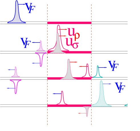
FIG. 2.: Dynamic transmission of an incident electron with spin up. The charge and spin (hatched) are separated even in the noninteracting leads. As an example, we consider here $u_{\rho}>u_{\sigma}$ , $K_{\sigma}<1$, $K_{\rho}>1$.

C ”Phase diagram”

In an infinite wire, interacting electrons with spin have a quite involved “phase diagram”; here we do not intend to study it entirely when the wire is connected to leads. We give some qualitative results and then discuss thoroughly the tendency towards the formation of a Wigner crystal. As for spinless electrons, we expect the dominant tendency to extend towards the leads in analogy with the proximity effect, but the leads can also intervene in the competition as will be shown later, especially at low enough temperature.

Let us first discuss the case where superconducting order can take place, as is the case in an infinite wire with $K_{\rho}>1$. One has to distinguish singlet SS, corresponding to the spin gap case, $K_{\sigma}^{*}=0$ and triplet SS, $K_{\sigma}^{*}=1$. If we naively take these values for $K_{\sigma}$ inside the wire, then we can show that:

For $K_{\sigma}^{*}=0$ inside the wire in order to take into account the spin gap, we can show that the tendency towards singlet super-conductivity holds for $K_{\rho}>1$, but the proximity effect towards the external leads shows up only for $K_{\rho}>3$. Remarkably, for $K_{\rho}\gg 1$, an incident electron with spin up is reflected back into one hole with spin down, and two quasi-particles of opposite spin, of charge unity and moving at velocity $u_{\rho}$ are transmitted, recalling Andreev reflection. [7, 16]

For $K_{\rho}>1$, and $K_{\sigma}^{*}=1$, we can show that triplet superconductivity develops and extends towards the external leads, but the Andreev reflection is more subtle to interpret.[16]

In the following, we focus on the situation $K_{\rho}<1$, $K_{\sigma}^{*}=1$, as it should be for quantum wires, and determine the dominant CDW in the density–density correlation function.

1 Density–density correlations

Let us compute the density-density correlation function. In order to express the density, we can superpose eq. (2) for the spin up or down, thus with the additional index $\nu=\rho$ or $\sigma$, then express $\Phi_{\nu}$ as function of $\Phi_{\rho},\Phi_{\sigma}$. This yields

$$\rho(x)=-\partial_{x}\left[\widetilde{\Phi}_{\rho}+\sum_{m_{\rho}\neq 0,m_{\sigma}}\frac{1}{2im_{\rho}}e^{i\sqrt{2}\left(m_{\rho}\widetilde{\Phi}_{\rho}+m_{\sigma}\Phi_{\sigma}\right)}\right],$$ (53)

where the sum runs over integers $m_{\rho}$ and $m_{\sigma}$ of the same parity,[5] and $\widetilde{\Phi}_{\rho}=\Phi_{\rho}-k_{F}x$. Normally only $m_{\rho}=\pm m_{\sigma}$ are allowed. But the other harmonics with $m_{\rho}\neq m_{\sigma}$ are generated by renormalization in the induced density that develops as a response to an external perturbation.[16]

The fermionic correlation functions can be expressed through the bosonic correlation function $U_{\nu}$ (and its dual) for $\nu=\rho,\sigma$ as in eq.(7) with $u(x)$ and $K(x)$ indexed by $\nu$. Then the density–density correlation function is similar to eq.(5) if one adds the subscript $\rho$ to $U$ in the first line, and $X_{m}$ is replaced by $X_{m_{\rho},m_{\sigma}}$ obtained from eq.(9) by the following substitution

$$2m^{2}U\rightarrow m_{\rho}^{2}U_{\rho}+m_{\sigma}^{2}U_{\sigma}.$$ (54)

Thus

$$X_{m_{\rho},m_{\sigma}}=\sqrt{X_{m_{\rho}}X_{m_{\sigma}}},$$

where $X_{m_{\nu}}$ is the analogous of $X_{m}$ without spin with $u$ and $K$ indexed by $\nu$. The imaginary part of the Fourier transform of $X_{m_{\rho},m_{\sigma}}$ at low frequencies, $\chi_{m_{\rho},m_{\sigma}}$ is defined as in eq.(10). It cannot be factored unless the spin and charge velocities are equal. For studying the dominant tendency, it is sufficient to consider its local values. Up to a slowly varying function of $x$, we have

$$\chi_{m_{\rho},m_{\sigma}}(x,x)=\sqrt{\chi_{m_{\rho}}(x,x)}\sqrt{\chi_{m_{\sigma}}(x,x)},$$ (55)

where $\chi_{m_{\nu}}(x,x)$ is exactly that computed without spin, with the additional index $\nu$, in particular there are two thermal lengths associated with the different charge and spin velocity $L_{T,\nu}=u_{\nu}/T$, two temperatures $T_{L,\nu}=u_{\nu}/L$, and two times (in units of $\tau_{0}$)

$$t_{x,\nu}=\frac{a-|x|}{u_{\nu}\tau_{0}}$$

for a spin ($\nu=\sigma$) or charge ($\nu=\rho$) excitation to go from $x$ to the closest contact.

The calculation can be carried out for any parameters for charge and spin, on the leads or inside the wire, but let us specify eq.(55) for non interacting leads, and for $K_{\sigma}=1$. In the high temperature limit, using eq.(23),

$$\chi_{m_{\rho},m_{\sigma}}(x,x) = \underline{T}^{m_{\rho}^{2}K_{\rho}+m_{\sigma}^{2}-2}(\tanh{}\underline{T}t_{x})^{m_{\rho}^{2}\gamma_{\rho}K_{\rho}}.$$ (56)

In particular, at a distance much greater than $L_{T,\rho}$ from the contacts, $\chi_{m_{\rho},m_{\sigma}}(x,x)$ is the same as that in an infinite wire

$$\chi_{m_{\rho},m_{\sigma}}(x,x)\sim\underline{T}^{m_{\rho}^{2}K_{\rho}+m_{\sigma}^{2}-2}.$$ (57)

For $m_{\rho}^{2}K_{\rho}+m_{\sigma}^{2}<2$, the $(m_{\rho},m_{\sigma})$ component of the density–density correlation function is enhanced compared to the noninteracting case.

In the low temperature limit, using eq.(24)

$$\chi_{m_{\rho},m_{\sigma}}(x,x)=\underline{T}^{m_{\rho}^{2}+m_{\sigma}^{2}-2}\underline{T}_{L\rho}^{-m_{\rho}^{2}\gamma_{\rho}}t_{x,\rho}^{m_{\rho}^{2}\gamma_{\rho}K_{\rho}}.$$ (58)

Note that the superconducting correlation functions can be obtained in a similar fashion, one has to distinguish the triplet from the singlet superconducting tendency, and we refer to [16] for more details.

2 The suppression of the Wigner crystal

In an infinite wire, the $4k_{F}$ CDW, corresponding to Wigner crystal, dominates the $2k_{F}$ CDW for very repulsive interactions, more precisely for $K_{\rho}<1/3$ and $K_{\sigma}=1$ as one can inspect using eq.(57). We show here that the leads can induce also a proximity effect in the opposite sense, by suppressing the Wigner Crystal at low temperature. This tendency is even more important for long–range Coulomb interactions to which case one could extend qualitatively the results obtained here.

Our study without spin has shown that the enhancement of a $2k_{F}$ CDW persists with leads. We have also observed that the $2mk_{F}$ CDW are suppressed at low temperature due to the $T$ dependent term $T^{2(m^{2}-1)}$ in $\chi_{m}$; but this effect intervenes only when the backscattering potential is studied on resonance, because the $2k_{F}$ CDW dominates $2mk_{F}$ for $m\geq 2$.

With spin, one has to compare the $2k_{F}$ to the $4k_{F}$ CDW, thus the correlation functions $\chi_{m_{\rho},m_{\sigma}}$ corresponding respectively to $(m_{\rho},m_{\sigma})=(1,1)$ and $(2,0)$. The competition is much less trivial than without leads and is [35] discussed in detail in appendix C. Here we summarize the results, illustrated by figs.3 and 4.

We will focus on the $K_{\rho}<1/3$ case, since for $K_{\rho}>1/3$ the $2k_{F}$ CDW is dominant at any temperature. Then contrary to the infinite wire where the $4k_{F}$ dominates, we show here that there is a crossover temperature $T_{c}(x)$ from the $4k_{F}$ CDW to the $2k_{F}$ CDW as $T$ is lowered below $T_{c}(x)$. $T_{c}(x)$ decreases monotonically when $x$ varies from one contact to the center of the wire where it reaches its minimum value, interestingly given by the following power of $T_{L}$:

$$\underline{T}_{c}(0)=\underline{T}_{L}^{\frac{3}{2}(1-K_{\rho})}.$$ (59)

One can check that $T_{c}(0)<T_{L}$ because $K_{\rho}<1/3$. Indeed $T_{c}(x)$ saturates at $T_{c}(0)$ for all $x$ such that $a-|x|\sim a$, i.e. $t_{x}T_{L}\sim 1$.

FIG. 3.: The case $K_{\rho}<1/5$: the Wigner crystal is suppressed below the crossover temperature $T_{c}(x)$, eq.(C6).

FIG. 4.: The same as fig.3, but with $1/5<K_{\rho}<1/3$.

Thus for any $T<T_{c}(0)$, the Wigner crystal is suppressed all over the wire and the dominant tendency is towards the $2k_{F}$ CDW.

In order to discuss the case $T>T_{c}(0)$ we shall investigate in detail the behavior close to the contacts. There is a second particular value other than $1/3$ that arises: all the correlation functions at $\pm a$ are analogous to those in the center of the wire with $K_{\nu}$ replaced by $K_{\nu a}=2K_{\nu}/(1+K_{\nu})$ (the analogue of eq.(20) with the supplementary index $\nu=\rho,\sigma$). When $K_{\sigma}=1$, $K_{a\sigma}=1$, the limiting value $K_{a,\rho}=1/3$ corresponds to $K_{\rho}=1/5$. In particular, as long as $K_{\rho}>1/5$ one has $K_{a,\rho}>1/3$, thus the $2k_{F}$ CDW dominates the $4k_{F}$ CDW at the contacts at any temperature.

This yields different expressions for $T_{c}(x)$ depending on $K_{\rho}$:

• For $1/5<K_{\rho}<1/3$, it is given by eq.(C8), and diverges at $\pm a$; reassuringly, we find that $T_{c}(x)$ is continuous at the point $x_{0}$ [eq.(C7)] where it reaches $T_{L}$ from below or above (fig.4).

• For $K_{\rho}<1/5$, $T_{c}(x)$ is given by Eq.(C6). $T_{c}(x)$ is below $T_{L}$ for any $x$, and reaches its maximum value at $a$; $T_{c}(a)$ is similar to eq.(59) where $K_{\rho}$ is replaced by $K_{a\rho}$. (fig.3)

If we consider now any $K_{\rho}<1/3$ and a given temperature in the range $[T_{c}(0),T_{c}(a)]$ ($T_{c}(a)$ is infinite for $K_{\rho}>1/5$), we see that the dominant tendency switches from the $4k_{F}$ to the $2k_{F}$ CDW when one goes from the center to the contacts. The point $x$ at which this transition occurs is a temperature dependent function $x_{c}(T)$ that is the inverse of $T_{c}(x)$. For $T$ higher than $T_{c}(a)$ (lower than $T_{c}(0)$), the $4k_{F}$ ($2k_{F}$) CDW dominates all over the wire.

To conclude, the external leads suppress the importance of the $4k_{F}$ CDW at low enough temperature or close to the contacts, thus preventing the tendency towards the formation of a Wigner crystal.

D Backscattering by non–random impurities

The role of impurities when spin is taken into account can be treated in a similar fashion as without spin, by doubling the indices as above, leading to different powerlaws on temperature. Nevertheless, in view of our previous discussion, the main additional complication arises from the competition between the $2k_{F}$ and $4k_{F}$ backscattering: the leads intervene more strongly if $K_{\rho}<1/3$.

We will first derive briefly the renormalization equations at finite temperature, then give results for the conductance.

The coupling to impurities is described in terms of $\int\rho(x)V(x)$, where $\rho$ is given by eq.(53). For any potential, the partition function can be expanded in terms of $V^{\prime}$ in a similar way as for the spinless case [eq.(27)], but with $m_{i}$ replaced by a couple of integers $(m_{\rho,i},m_{\sigma,i})$. Then $Z$ describes integer charges restricted to two neutral cylinders, corresponding to the charge ($\nu=\rho$) and the spin ($\nu=\sigma$) degree of freedom. The radius of each cylinder is given by $\beta/\pi$, and its height determined by the spatial extension of the potential. Only charges on the same cylinder $\nu$ interact via $U_{\nu}(x,y,\tau)$, eq.(7) with the index $\nu$ on any function or parameter.

Following similar steps as in the spinless case, we can infer the leading renormalization equation analogous to (28), where $U$ is replaced according to the recipe (54),

$$\frac{dV^{\prime}(x.m_{\rho},m_{\sigma})}{dl} = \left[1-\frac{1}{2}\left(m_{\rho}^{2}\frac{dU_{\rho}}{dl}+m_{\sigma}^{2}\frac{dU_{\sigma}}{dl}\right)\right]V^{\prime}.$$ (60)

For simplicity we have omitted the arguments on the right hand side. In particular, through $U_{\nu}$, $V$ now acquires an additional spatial dependence.

The bare value of $V(x,m_{\rho},m_{\sigma})$ is zero if these terms are not present in the initial density representation, eq.(53). In order to illustrate how they are generated, we specialize to the case of one barrier. Then the cylinders shrink to circles, and the partition function reads

$$Z = \sum_{n}(-1)^{n}\int_{(n-1)\tau_{0}}^{\beta-\tau_{0}}{d\tau_{n}}\ldots\int_{0}^{\tau_{2-}\tau_{0}}{d\tau_{1}}$$ (62)

$$\sum_{\sum_{i}m_{\nu i}=0}\prod_{i=1}^{n}V_{m_{\rho i},m_{\sigma i}}\exp\left[{\sum_{i\neq j,\nu}m_{\nu i}m_{\nu j}U_{\nu}\left(\tau_{i}-\tau_{j}\right)}\right].$$

The sum runs over all $n$-tuples of integers $m_{\rho i}$ and $m_{\sigma_{j}}$ with total vanishing sum separately, and the bare transform of $V$

$$V_{m_{\rho},m_{\sigma}}=\int V^{\prime}(x)e^{2im_{\rho}\phi_{0}(x)}$$ (63)

acquires a dependence on $m_{\sigma}$ during renormalization. We can show that the interactions are not renormalized as for the spinless case. The next–leading term to eq.(60) is obtained by the contraction of one pair of charges on each circle, and is equal to[16]

$$\sum V(n_{\rho},n_{\sigma})V(n^{\prime}_{\rho},n^{\prime}_{\sigma}),$$ (64)

up to non universal prefactors, the sum running over $n_{\rho}+n^{\prime}_{\rho}=m_{\rho}$ and $n_{\sigma}+n^{\prime}_{\sigma}=m_{\sigma}$.

For a potential with extension $d$ much less than $L$ and $L_{T}$, we can show that the partition function is analogous to eq.(62) when a cutoff larger than $d$ is reached. Again, at the location of $V$ the interaction parameters might be renormalized before reaching this stage.

If the renormalization of the local effective interactions, as well as next leading terms can be ignored, eq.(60) can be integrated easily. The maximum cutoff is half the radius of one cylinder, i.e. $\beta/2$, where we get the renormalized parameters[36]

$$V^{\prime}(x;m_{\rho},m_{\sigma})=V^{\prime}(x)\chi_{m_{\rho},m_{\sigma}}(x,x).$$

$\chi_{m_{\rho},m_{\sigma}}(x,x)$ has been studied previously, and is given by eq.(56) (respectively (58)) in the high (low) temperature limit.

For $K_{\sigma}=1$, $K_{\rho}<1$, and for any $x$, $V^{\prime}$ is enhanced when the temperature is lowered, and is less enhanced when one gets closer to the contacts because the leads moderate the repulsive interactions. If the potential is weak enough or the wire is short enough, we can perform the renormalization at temperatures below $T_{L}$. The renormalized $V^{\prime}(x,1,1)$ obtained at a given $T<T_{L}$ is the same for all $T<T_{L}$, but this is not the case for all the other couples $(m_{\rho},m_{\sigma})\neq(1,1)$, for which $V^{\prime}(x,m_{\rho},m_{\sigma})$ goes down to zero at zero temperature. For instance, we refer to our previous discussion of the competition between the $2k_{F}$ and $4k_{F}$ backscattering contribution.

Now we give the perturbative expression for the conductance. For a general weak potential $V(x)$, the conductance can be expressed as in eq.(36). $\mathcal{R}$ is similar to eq.(37) with $m$ standing for a couple of integers $m_{\rho},m_{\sigma}$ with the same parity. This substitution applies also to eq.(38), giving

$${\mathcal{R}}_{m_{\rho},m_{\sigma}} = \int\-\-\-\int\frac{V^{\prime}(x)V^{\prime}(y)}{(k_{F}u)^{2}}e^{2im_{\rho}\left[\phi_{0}(x)-\phi_{0}(y)\right]}\chi_{m_{\rho},m_{\sigma}}(x,y).$$ (65)

The nonlocal function $\chi_{m_{\rho},m_{\sigma}}(x,y)$ is now more difficult to compute due to the different velocities of spin and charge. But if we assume $u_{\rho}=u_{\sigma}$, it can be inferred from that without spin (see appendix B) by replacing

$$2m^{2}K\rightarrow m_{\rho}^{2}K_{\rho}+m_{\sigma}^{2}K_{\sigma}.$$

When the potential has an extension less than $L$ and $L_{T,\nu}$ ($\nu=\rho,\sigma$), only the local value is required as far as the dominant term is concerned.[32] Then the leading term is similar to eq.(39) with $m$ replaced by the pair $(m_{\rho},m_{\sigma})$, thus replacing $V_{m}$ by eq.(63), and using Eqs. (56,58).

For $K_{\rho}<1/3$, we refer to figures 3 and 4. Above (below) the crossover temperature $T_{c}(x)$, where $x$ is the location of the barrier, the $4k_{F}$ (respectively $2k_{F}$) backscattering gives the dominant contribution, and can be inferred from Eqs. (56,58) by taking $(m_{\rho},m_{\sigma})=(1,1)$ (respectively $(2,0)$) depending on whether $T<T_{L}$ or $T>T_{L}$.

E Extended disorder: Conductance fluctuations

For a random potential verifying eq.(40), the leading term of $\mathcal{R}$ is given explicitly in figure 5. Again the case $K_{\rho}<1/3$ is more complicated: we have to distinguish three temperature regimes, separated by $T_{L}$ than $T_{c}(0)$, eq.(59).

We can also compute the variance of $\mathcal{R}$, using Eqs. (65,40). Similar steps to that without spin can be carried on. While the powerlaw behavior of $Var({\mathcal{R}})$ is different from that without spin, the relative fluctuations are the same, i.e. we have still eq.(47) in the low temperature limit, and eq.(50) (with a different function $I$ that does not affect the order of magnitude) in the high temperature limit.

Let us give the behavior of $Var({\mathcal{R}})$. In the low temperature limit $T<T_{L}$, the inequality (46) holds again, showing that $Var({\mathcal{R}})$ is of the same order as ${\mathcal{R}}^{2}$, eq.(47), given in fig.5. In particular, in the case $1/3<K_{\rho}<1$,

$$\sqrt{Var({\mathcal{R}})}\simeq\frac{u\tau_{0}}{l_{e}}\underline{T}_{L}^{2-K_{\rho}}.$$

For $K_{\rho}<1/3$, this powerlaw holds at lower temperature $T<T_{c}(0)$, eq.(59), but

$$\sqrt{Var{\mathcal{R}}}\simeq\frac{u\tau_{0}}{l_{e}}\underline{T}^{2}\underline{T}_{L}^{4K_{\rho}-5}$$

for $T_{c}(0)<T<T_{L}$.

In the high temperature limit $T>T_{L}$, restricting ourselves to $K_{\rho}<1$, we can retain only the contribution of the bulk. Then we find

$$Var({\mathcal{R}})\sim\frac{u_{\rho}\tau_{0}L}{l_{e}^{2}}\underline{T}^{m_{\rho}^{2}K_{\rho}+m_{\sigma}^{2}K_{\sigma}-3},$$ (66)

up to a bounded function of both $k_{F}L_{T\nu}$ for $\nu=\rho,\sigma$. Again, we have ignored the terms due to first and second derivatives of $\chi$, and kept only the pair $(m_{\rho},m_{\sigma})$ that yields the dominant term. This pair is equal to $(1,1)$ (respectively to $(2,0)$) for $K_{\rho}>1/3$ (respectively $K_{\rho}<1/3$) as is the case for the dominant contribution to $\left\langle\mathcal{R}\right\rangle$. Remarkably, the ratio (50) is the same as that without spin up to the function $I$, and is $\ll 1$ in any parameter range.

IV Discussion and Generalizations

Different aspects of transport in an interacting wire with measuring leads have been treated in this paper. In this section, we will compare the effect of backscattering on the conductance to that obtained without leads, and then discuss the results that can be generalized to smooth variations of the interactions at the contacts.

In an infinite wire with repulsive interactions, as is thought to be appropriate for a quantum wire, a unique local barrier is sufficient to suppress transport completely.[2, 5] The finite length is intuitively introduced as a cutoff, thus preventing the conductance to vanish for weak enough backscattering potential or short enough wire.[4, 5, 37] With noninteracting leads and spinless electrons, we recover the results of refs.[37, 5] over all the temperature range only for a barrier whose separation from the contacts is of the order of the wire length $L$, and under the additional condition $K_{\rho}>1/3$ for electrons with spin.

If we consider extended disorder, the agreement holds for $K<(3+\sqrt{1}7)/2$ without spin, and for $1/3<K_{\rho}<1+\sqrt{2}$ with spin (see fig 5). In this parameter range, the localization length we infer from the breakdown of our perturbative evaluation of $\mathcal{R}$ coincides with that found in ref.[3] in the weak disorder limit.

We now discuss the extension of our results to smooth variations. As we mentioned before, the discontinuous parameter model can be relevant for edges states in the FQHE[19, 20], but is not well justified microscopically for quantum wires. Thus it is important to know which results can be trusted for a more realistic interaction profile.

The detailed behavior of the transmission dynamics of an incident electron was given previously for abrupt jumps.[7, 13] By inspecting the boson Green function, we can maintain the qualitative conclusion; in particular, the transmitted charge and spin stay separated in the external leads.

The correlation functions are directly related to this process.[16] All the properties of $\chi$ found in subsection II B 1 still hold. To be specific, assume that the leads are non interacting, $K_{L}=1$ and that $K$ decreases slowly enough from $1$ to its bulk value $K$ inside the wire. Again, for $K<1$, [cf. Eqs. (13) and (14)] the tendency towards the CDW holds inside the wire, but is reduced when one goes to the leads, until it reaches its noninteracting value in the leads at a distance $u/(\omega K)$ where $\omega$ is the maximum energy at hand, recalling the proximity effect. Analogous conclusions hold for the superconducting fluctuations when interactions are attractive, the coherence length being now $uK/\omega$.

In the presence of a non–random backscattering potential, the renormalization equations (60) are general. The role of backscattering is determined by the density–density correlations. Consider for instance a barrier at a point $x$. When $x$ is at a distance of order $L$ of the contacts, the role of backscattering is the same as that in ref.[5]. For $K<1$, $\mathcal{R}$ (see Eqs. (14) and (39)) decreases when $x$ gets closer to the contacts. The noninteracting leads (where a barrier is marginal) tend to reduce the importance of the repulsive interactions when one gets closer to them. Using the boson Green function properties on the external leads (restricting ourselves to the case $K_{\sigma}=1$ with spin), the temperature dependence of the correlation function corresponding to the $2mk_{F}$ CDW at $T<T_{L}$ has a term $T^{m^{2}K_{L}-1}$. Thus for $K_{L}=1$, this saturates for $m=1$ but goes to zero at zero temperature for $m\neq 1$. In particular, the usual scaling argument inferring the low temperature behavior $T<T_{L}$ from that at $T>T_{L}$ is justified only if the $2k_{F}$ contribution intervenes at all temperatures, which is not the case in our model for spinful electrons with $K<1/3$, or for any parameter range when the resonance in the presence of backscattering potential is achieved.

For a random potential, all the results can be generalized for repulsive interactions. But the inequality (46) is more general than that, and holds even if $K$ varies in any way inside the wire.

When spin is taken into account, and for $K_{\sigma}=1$, the tendency towards a Wigner crystal is expected to be suppressed at low temperature, more precisely the dominant tendency is that towards the $2k_{F}$ CDW at any $T<T_{c}(0)$ [eq.(59)]. This is because the dependence on temperature of the $4k_{F}$ CDW is controlled by $K_{L}=1$, thus is in $T^{4K_{L}-1}=T^{3}$, vanishing in the zero temperature limit.

In the presence of Coulomb interactions, the ballistic conductance is still independent on the interactions.[23, 16, 12] One can make an analogy with the case $K_{\rho}<1/3$ to expect the transmitted charge and spin to stay separated in the leads, and the tendency towards Wigner Crystal to be suppressed by the leads at low enough temperature.

V Experiments

We now comment on the experimental situation. In the high–temperature limit, the ballistic value of the conductance of one-channel quantum wire $2e^{2}/h$ was observed by Tarucha et al.,[10] as well as in the remarkable clean wires of Yacoby et al.[11] But the low temperature behavior is more tricky.

On the one hand, Tarucha et al. fitted the observed $\mathcal{R}$ with the intuitive law $[T^{2}+T_{L}^{2}]^{(K_{\rho}-1)/2}$ of ref.[37], and infer the parameter $K_{\rho}=0.7$. We however find a more complex dependence of $\mathcal{R}$ on the temperature and the location of the barriers. For instance, if the backscattering is merely due to the contacts, the exponent $0.7$ would correspond to the local parameter $K_{a\rho}=2K_{\rho}/(1+K_{\rho})$, thus to $K_{\rho}\approx 0.5$. Of course we don’t expect the same combination of parameters to appear in the case of smooth variations of $K$, but this serves as an illustration; as we discussed in section IV, the effective parameter that controls the powerlaw increases when one gets closer to the wire. Probably the potential configuration depends on each wire, and more precise fit and evaluation of $K_{\rho}$ are required. Even more caution is needed if the potential is random. While the conductance is self–averaging at high temperature (eq.(50)), its fluctuations become more important at low temperature, of the order of the reduction $\mathcal{R}$, eq.(47); then one has not to measure simply the absolute value of $\mathcal{R}$, but also its fluctuations.

On the other hand, Yacoby et al.[11] fabricated high quality quantum wires using a sophisticated technique. The most striking result is that the conductance shows perfect plateaus as function of the gate voltage. Their value is $Ge^{2}/h$ per spin mode and channel where $G\leq 1$. $G$ depends on the temperature and the wire length, but is reproducible for different wires made in wells of the same width. This indicates that the reduction in the conductance is not due to potential fluctuations, but rather to the backscattering of electrons from the two–dimensional gas when entering the wire. In the high temperature limit, the one-channel wire conductance is $e^{2}/h$, ($G=1$) in accordance with theoretical results. But $G$ decreases when one lowers temperature, or increases the wire length, in a way similar qualitatively to the law $T^{K-1}$ or $L^{1-K}$ for an interacting wire with parameter $K$. The main objection of Yacoby et al. against this TLL interpretation is that temperature is scaled by the Fermi energy which varies with electron density, in contradiction with the observed plateaus which are density independent. Further, the parameter $K$ itself is expected to depend on the density.

The importance of these two effects is however not so obvious to assess. First, energy scales different from the Fermi energy might play the role of the cutoff. Second the way $K$ depends on the density (i.e. the gate voltage) is difficult to estimate: a fully microscopic calculation of $K$ would be necessary, including the capacitive effects of the gates. We have however also to remark that our model is not the best suited to describe the complicated geometry of the experiments. The transition between the two–dimensional gas and the wire is not easy to describe, and is different from the usual adiabatic transition. Thus we think model closer to the actual experiment needs to be developed.[38]

VI Summary

In this paper we have studied the properties of an interacting wire connected to measuring leads. We have obtained a number of new results, mainly concerning the suppression of the Wigner crystal and its effect on the conductance with impurities, and the conductance fluctuations. We have also completed our study of the transmission process by taking spin into account. We have shown here that the clean wire acts as a separator of the charge and spin of an incident electron, which don’t recombine in the noninteracting leads. We can hope that experimental progress allows this feature to be observable by appropriate spin and charge detectors. We have also given a systematic computation of the nonlocal correlation functions and their Fourier transform at temperature $T\gg\omega$. This has allowed to investigate both the dominant tendency in and outside the wire and to study the role of impurities.

As first mentioned in ref.[7], we have explained in more detail how the proximity effect shows up. For repulsive (attractive) interactions, the charge density (pairing) fluctuations are enhanced in the bulk of the wire, and decrease, while staying enhanced compared to the noninteracting case, when one goes beyond the contacts. But the novel effect is that the leads influence the competition between different tendencies in the wire at low enough temperature. This was shown to be the case for very repulsive short range interactions $K<1/3$. Normally, a tendency towards a Wigner crystal shows up, corresponding to the $4k_{F}$ CDW. When connected to leads, such tendency gets suppressed below a space-dependent crossover temperature, and is replaced by the $2k_{F}$ CDW. In particular, this allows for simultaneous $2k_{F}$ and $4k_{F}$ CDW in the wire in a certain temperature range. $T_{c}$ is controlled by interactions, thus its measurement could provide a way to measure $K$. The Wigner crystal shows up more strongly for Coulomb interactions; we have not studied this case, but we expect the same qualitative conclusions to hold.

We have also studied the role of a backscattering potential. We have developed a formal framework to study its role for any non–translationally invariant interactions, and explicitly at finite temperature. We have derived the renormalization equations for a non–random potential $V$ with any extension, but we expect interactions to be renormalized by a nonlocal $V$. If $V(x)$ is weak enough for this effect to be neglected, the conductance $g$ was expressed in detail in the discontinuous parameter case. $g$ is controlled by the interactions, but is influenced by the external leads, especially for very repulsive interactions because the leads suppress the tendency towards the Wigner crystal below $T_{c}(x)$ [cf Figs. 3,4]. We have computed the conductance fluctuations, whose behavior is nonuniversal. But remarkably, the ratio $Var({\mathcal{R}})/{\mathcal{R}}^{2}$ stays of the same order, whether the spin is taken into account or not, or whether $K>1/3$ or not. It is $\sim 1/2$ for $T<T_{L}$, and $\sim L_{T}/L\ll 1$ for $T>T_{L}$. We can generalize the main results to a smooth interaction profile near the contacts.

One of us (I. S.) would like to thank B. Douçot, D. C. Glattli, T. Martin, D. L. Maslov and A. Yacoby for interesting discussions.

A Formal expression for the conductance

We derive the analogue of a Dyson equation for the nonlocal conductivity. We begin by spinless electrons, taking into account spin will the be straightforward. We consider a general Hamiltonian

$$H_{tot}=H+{\mathcal{V}}(\Phi),$$ (A1)

where $H$ is given by eq.(1), and ${\mathcal{V}}(\Phi)$ depends on $\Phi$, but not on its conjugate canonical momentum $\Pi=\partial_{x}\Theta/\pi$. Let us first give the general equation of motion for $\Phi$. Using $\left[\Pi(x),\Phi(y)\right]=i\delta(x-y)$, any functional $\mathcal{F}$ of $\Phi$ verifies

$$\left[\Pi,{\mathcal{F}}\right]=-i\frac{\partial{\mathcal{F}}}{\partial\Phi}.$$ (A2)

This allows us to write the system

$$\left\{\begin{array}[]{c}\partial_{t}\Phi=\frac{\partial H_{tot}}{\partial\Pi}=\pi uK{\Pi}\\ \partial_{t}\Pi=-\frac{\partial H}{\partial\Phi}=\frac{1}{\pi}\partial_{x}\left(\frac{u}{K}\partial_{x}\Phi\right)+{\cal I},\end{array}\right.$$ (A3)

where

$${\cal I}(x)=\frac{\partial{\mathcal{V}}(\Phi)}{\partial\Phi(x)}$$ (A4)

Note that $uK\mathcal{I}$ has the dimension of a force that intervenes in the time derivative of $j=uK\Pi$. Eliminating ${\Pi}$ in eq.(A3), the equation of motion for $\Phi$ reads

$$D_{xt}\Phi={\cal I},$$ (A5)

where we denote

$$D_{xt}=\frac{1}{\pi}\left[-\partial_{tt}+uK\partial_{x}\left(\frac{u}{K}\partial_{x}\right)\right].$$ (A6)

For an arbitrary nonlocal interaction potential $U(x,y)$, $D_{xt}$ contains also an integral operator,[12, 16] and all the remaining analysis can be generalized to that case.

Note that without $\mathcal{V}$, we have ${\cal I}=0$, and thus recover the equation of motion $D_{xt}\Phi=0$. In the following, the corresponding correlation functions carry a subscript $0$, in order to distinguish them from those computed with ${\cal V}$.

Next we derive a Dyson equation for the nonlocal conductivity ${\cal I}$, eq.(A4). For any $A$ depending on $\Phi$ in a local or nonlocal way, we can show, using eq.(A2) and eq.(A5), that

$$D_{xt}\left\{-i\theta(t)\left\langle\left[\Phi(x,t),A\right]\right\rangle\right\}=i\theta(t)\left\langle\left[{\cal I}(x,t),A\right]\right\rangle+\delta(t)\frac{\partial A}{\partial\Phi(x)}$$ (A7)

where $\theta$ is the Heaviside function. The Fourier transform with respect to time of eq.(A7) yields

$$D_{x\omega}\left\langle\left\langle\Phi(x);A\right\rangle\right\rangle_{\omega}=\left\langle\left\langle{\cal I}(x);A\right\rangle\right\rangle_{\omega}+\frac{\partial A}{\partial\Phi(x)},$$ (A8)

where we adopt the notation [39]

$$\langle\langle A(x);B(y)\rangle\rangle_{\omega}=-i\int_{0}^{\infty}e^{i\omega t}\left\langle\left[A(x,t),B(y,0)\right]\right\rangle_{H_{tot}}.$$ (A9)

We point out that the correlation functions are defined here with the total Hamiltonian $H_{tot}$, eq.(A1). Similarly, we can show that

$\displaystyle D_{y\omega}\left\langle\left\langle A;\Phi(y)\right\rangle\right\rangle_{\omega}=\left\langle\left\langle A;I(y)\right\rangle\right\rangle_{\omega}+\frac{\partial A}{\partial\Phi(y)}.$

Applying these two identities successively to the Green function

$$G(x,y,\omega)=\left\langle\left\langle\Phi(x);\Phi(y)\right\rangle\right\rangle_{\omega},$$

we get

$\displaystyle D_{y\omega}D_{x\omega}G(x,y,\omega)=D_{y\omega}\delta(x-y)+\frac{2i\omega}{\pi}f(x,y,\omega)$

where $f$ denotes

$$f(x,y,\omega)=\frac{\pi}{2i\omega}\left[\left\langle\left\langle{\cal I}(x);{\cal I}(y)\right\rangle\right\rangle_{\omega}+\frac{\partial{\cal I}(x)}{\partial\Phi(y)}\right].$$ (A10)

In order to invert the relation above, and thus to obtain $G_{I}(\overline{x},\overline{y},\omega)$ where $\overline{x},\overline{y}$ are arbitrary, we multiply its two members by $G_{0}(\overline{y},y,\omega)$, integrate over $y$, and use

$$D_{y\omega}G_{0}(\overline{y},y,\omega)=\delta(y-\overline{y}).$$

Then we multiply both sides by $G(\overline{x},x,\omega)$ and integrate over $x$. We get

$$G(\overline{x},\overline{y},\omega) = G_{0}(\overline{x},\overline{y},\omega)+\frac{2i\omega}{\pi}\int\-\int dxdy$$ (A12)

$$G_{0}(\overline{x},x,\omega)G_{0}(\overline{y},y,\omega)f(x,y,\omega).$$

We can also express this equation in terms of the dimensionless nonlocal conductivity (measured in units of $e^{2}/h$), eq.(34):

$$\sigma(\overline{x},\overline{y},\omega) = \sigma_{0}(\overline{x},\overline{y},\omega)-\int\int dxdy$$ (A14)

$$\sigma_{0}(\overline{x},x,\omega)\sigma(\overline{y},y,\omega)f(x,y,\omega).$$

The conductance measured in units of $e^{2}/h$ is given by eq.(35),

$$g=\lim_{\omega\rightarrow 0}\sigma(\overline{x},\overline{y},\omega)=\sigma(\overline{x},\overline{y})$$ (A15)

independent of its arguments, which ensures current conservation. It is also real because it is a correlation function of two Hermitian fields. Indeed, for two hermitian operators $A,B$, we have

$$\left(\left\langle\left\langle A;B\right\rangle\right\rangle_{0}\right)^{\dagger}=i\int_{0}^{\infty}\left\langle\left[B^{\dagger},A^{\dagger}\right]\right\rangle=\left\langle\left\langle A;B\right\rangle\right\rangle_{0}\;\;\;\mbox{real}.$$

Besides,

$\displaystyle\frac{d}{d\omega}\left\langle\left\langle A;B\right\rangle\right\rangle_{\omega=0}=\int_{0}^{\infty}t\left\langle\left[A,B\right]\right\rangle dt\;\;\;\mbox{is purely imaginary}$

Thus $\lim_{\omega\rightarrow 0}\left\langle\left\langle{\cal I}(x);{\cal I}(y)\right\rangle\right\rangle_{\omega}$ is real while its derivative at zero frequency is purely imaginary because ${\cal I}$ is hermitian. If one supposes $\sigma{}(\overline{x},\overline{y})$ finite, one has

$\displaystyle\int dx\int dy\left[\left\langle\left\langle{\cal I}(x);{\cal I}(y)\right\rangle\right\rangle_{0}+\frac{\partial{\cal I}(x)}{\partial\Phi(y)}\right]=0.$

Then the zero frequency limit of eq.(A14) yields the exact conductance measured in units of $e^{2}/h$

$\displaystyle g=g_{0}\left[1-g_{0}\int dx\int dyf(x,y)\right].$

where

$\displaystyle f(x,y)=\frac{\pi}{2}Im\frac{d}{d\omega}\left\langle\left\langle{\cal I}(x);{\cal I}(y)\right\rangle\right\rangle_{\omega=0}$

is the zero–frequency limit of eq.(A10) and $g_{0}$ is the dimensionless conductance in the absence of $\mathcal{V}$. If one takes spin into account, ${\mathcal{V}}$ can depend on the spin field $\Phi_{\sigma}$ and its conjugate canonical momentum $\Pi_{\sigma}$, both commuting with the field $\Phi_{\rho}$. This is the case for instance for backscattering potential, where the contribution of the $(m_{\rho},m_{\sigma})$ harmonics of the density (53) to $\mathcal{I}$ reads, after integration by parts: $\int V^{\prime}(x)\exp\left({2im_{\rho}\widetilde{\Phi}_{\rho}+2im_{\sigma}\Phi_{\sigma}}\right)$.

B Correlation functions

We will show how to compute the imaginary part of the Fourier transform of the nonlocal correlation function (9) at frequency $\omega\ll T$, i.e. $\chi(x,y)$ [eq.(10)].

First we clarify the way analytic continuations from Matsubara to real frequencies are done when we regularize by imposing the imaginary time to obey $\tau_{0}\leq\tau\leq\beta-\tau_{0}$. Consider any general operators $A$ and $B$. Using the equivalent of the notation (A9) for the Matsubara frequency $i\omega_{n}$, we have

$$\langle\langle A;B\rangle\rangle_{i\omega_{n}} = \int_{\tau_{0}}^{\beta-\tau_{0}}e^{i\omega_{n}\tau}\left\langle A(\tau)B(0)\right\rangle$$ (B1)

$$= \int_{0}^{\infty}d(it)\left\{-e^{i\omega_{n}(it+\tau_{0})}\left\langle A(it+\tau_{0})B(0)\right\rangle\right.$$ (B3)

$$\left.+e^{i\omega_{n}(it+\beta-\tau_{0})}\left\langle A(it+\beta-\tau_{0})B(0)\right\rangle\right\}$$

$$= -i\int_{0}^{\infty}dte^{-\omega_{n}t}\left\{e^{i\omega_{n}\tau_{0}}\left\langle A(it+\tau_{0})B(0)\right\rangle\right.$$ (B5)

$$\left.-e^{-i\omega_{n}\tau_{0}}\left\langle B(-it+\tau_{0})A(0)\right\rangle\right\},$$

where we have deformed the integration contour in the complex plane, and used

$\displaystyle\left\langle A(\beta-z)B(0)\right\rangle=\left\langle B(z)A(0)\right\rangle$

Let us now specialize to the case

$$A=B^{\dagger}=e^{2im\Phi}$$

where $m$ is normally an integer but can be any real, and consider $X_{m}$, eq.(9)

$$X_{m}(x,y,\tau)=\left\langle T_{\tau}A^{\phantom{\dagger}}(x,\tau)A^{\dagger}(y,0)\right\rangle.$$ (B6)

Then we have

$$\left\langle T_{\tau}A(x,\tau)A^{\dagger}(y,0)\right\rangle=\left\langle T_{\tau}A^{\dagger}(x,\tau)A(y,0)\right\rangle.$$ (B7)

This is because the transformation: $\Phi\to-\Phi$ leaves $H$ invariant, but $A\to A^{\dagger}$. Besides, $X_{m}$ is invariant when exchanging $x$ and $y$ because of time reversal symmetry .

Equation (B1) becomes, after the analytic continuation $i\omega_{n}\rightarrow\omega+i\delta$,

$$X_{m}(x,y,\omega) = -i\int_{0}^{\infty}dte^{i\omega t}\left\{e^{\omega\tau_{0}}\left\langle A(x,it+\tau_{0})A^{\dagger}(y,0)\right\rangle\right.$$ (B9)

$$\left.-e^{-\omega\tau_{0}}\left\langle A^{\phantom{\dagger}}(x,-it+\tau_{0})A^{\dagger}(y,0)\right\rangle\right\}.$$

The derivative with respect to $\omega$ yields, after changing $t\to-t$ in the second term above,

$$\left.\frac{dX_{m}}{d\omega}\right|_{\omega=0}=-i\int_{-\infty}^{\infty}(it+\tau_{0})X_{m}(x,y,it+\tau_{0}),$$ (B10)

where $X_{m}(x,y,z)=\left\langle A(x,z)A^{\dagger}(y,0)\right\rangle$. According to eq.(B10), and after the change of variables $t\rightarrow\pi Tt$,

$$\left.-\frac{d\chi_{m}}{d\omega}\right|_{\omega=0}=\frac{1}{(\pi T)^{2}}\int_{-i\infty+\underline{T}}^{i\infty+\underline{T}}z\exp\left[-2m^{2}U(x,y,z)\right]dz,$$ (B11)

where $\underline{T}=\pi T\tau_{0}$, and $U$ is given by eq.(7).

Owing to the analytic properties of $U$, we can move the integration contour in eq.(B11) as explained now. Let us write the integral in eq.(B11) as

$$\int_{-i\infty+\underline{T}}^{i\infty+\underline{T}}zX_{m}(z),$$

where the spatial arguments are implicit. $U$ is analytic on the complex band $\underline{T}\leq{\rm Re}(z)\leq\pi/2$, as well as $zX_{m}(z)$.

Let $z=\mu+i\nu$. We then have $\underline{T}\leq\sin\mu\leq 1$. We can show that for $\nu\rightarrow\infty$,

$$X_{m}(z)\sim e^{-m^{2}K_{L}|\nu|}.$$

Then we can translate the contour of integration by $\pi/2-\underline{T},$ thus making it along $z=it+\pi/2$. On the other hand, we can show that $X_{m}(it+\pi/2)$ is an even function of $t$, thus

$$\int_{-\infty}^{+\infty}tX_{m}(it+\pi/2)=0.$$

Finally, the integral (B11) becomes

$\displaystyle-\left.\frac{dX_{m}}{d\omega}\right|_{\omega=0}=\frac{a}{2\pi T^{2}}\int_{-i\infty+\pi/2}^{i\infty+\pi/2}dze^{-2m^{2}U(z)}$

This form is much more convenient than (B11) for three reasons: the integrand is real, the singularities are avoided, and approximations are easier to make. Thus the dimensionless function $\chi$, eq.(10), corresponding to $m=1$ can be expressed as

$$\chi\left(x,y\right)=\frac{1}{2\underline{T}^{2}}\int_{-i\infty+\pi/2}^{i\infty+\pi/2}X(x,y,\tau)d\tau.$$ (B12)

This gives eq.(11):

$$\chi\left(x,y\right)=\frac{1}{\underline{T}^{2}}C(x,y)e^{-2G(x,x,\tau_{0})}e^{-2G(y,y,\tau_{0})},$$ (B13)

where

$$C(x,y)=\int_{0}^{\infty}d\zeta\exp\left[4G(x,y,i\zeta+\pi/2)\right].$$ (B14)

All the $\chi_{m}$ can be obtained by multiplying $G$ by $m^{2}$.

1 Discontinuous parameters

Let us give the function $G$ in the case of discontinuous interaction parameters[16]

$$-2G(x,y,z)/K=h\left(z,v_{-}\right)+\gamma h\left(z,v_{+}\right)+\sum_{r=\pm 1}\sum_{p=1}^{\infty}$$ (B16)

$$\left[\gamma^{2p}h\left(z,2pv_{L}+rv_{-}\right)+\gamma^{2p+r}h\left(z,2pv_{L}+rv_{+}\right)\right]$$

with

$$h(z,v)=\frac{1}{2}\log\left[\sin^{2}\pi Tz+\sinh^{2}v\right],$$ (B17)

and

$$v_{-} = \pi T\left|x-y\right|/u$$ (B18)

$$v_{+} = \pi T\left(L-\left|x+y\right|\right)/u$$ (B19)

$$v_{L} = \pi TL/u.$$ (B20)

$\gamma$ is given by eq.(19). It is worth noting that one can deduce $G$ from $\sigma(x,y,\omega)$ as explained in ref.[16], and that $\sigma(x,y,\omega)$ is related to the transmission process.[7]

a High temperature limit

Let us first consider the limit $T\gg T_{L}$. We can show in detail that a good approximation of the integral $C(x,y)$, eq.(B14), can be obtained if we approximate $G$ by

$$-2G(x,y,z)\simeq K\left\{h\left(z,v_{-}\right)+\gamma\left[h\left(z,v_{+}\right)-v_{+}+\log 2\right]\right\}.$$ (B21)

There is no coherence between the two contacts separated by $L\gg L_{T}$, so that only the role of one reflection matters. The integral can be expressed as

$$C\left(x,y\right) = \left(1+e^{-2v_{+}}\right)^{-2\gamma K}\frac{B\left(\frac{1}{2},K_{a}\right)}{2\cosh^{2K}v_{-}}$$ (B23)

$$F_{1}\left(\frac{1}{2},K,\gamma K,\frac{1}{2}+K_{a};\tanh^{2}v_{-},\tanh^{2}v_{+}\right),$$

where $F_{1}$ is the hypergeometric function generalized to two variables,[40] and $K_{a}$ given by eq.(20).

In the limit of an infinite wire with constant parameters, we can set $K=K_{L}$, i.e. $\gamma=0$. Then $C(x,y)$ is a function of $x-y$, or of $v$ [eq.(B20)] and becomes

$$C_{K}\left(v\right)=B(\frac{1}{2},K){{}_{2}F_{1}}\left(K,K,\frac{1}{2}+K;-\sinh^{2}v\right),$$ (B25)

where $B$ is the Beta function and ${}_{2}F_{1}$ is the hypergeometric function of one variable.

At distances far from the contacts compared to $L_{T}$, thus for $v_{+}\gg 1$, we have

$$C(x,y)\simeq C_{K}(v_{-}).$$

In order to express $\chi$, eq.(B13), we need also to exponentiate eq.(B21) for $x=y$, and $z=\tau_{0}$. Thus one gets $\chi(x,y)$ for any $x,y$.

a Local value

For $|x-y|\ll L_{T}$, we can check that $C(x,y)\simeq C(x,x)$. Nevertheless, for $e^{-2G(x,x,\tau_{0})}\simeq e^{-2G(y,y,\tau_{0})}$ to hold, we must have $t_{x},t_{y}\gg 1$. Thus strictly speaking the property (17) (now $L_{min}=L_{T}$ since we are in the high temperature limit) holds only for $t_{x}\gg 1,t_{y}\gg 1$. But this is related to the abrupt jump of parameters at the contacts, thus we don’t expect it to hold for smooth variations, where eq.(17) can be generalized. Besides bosonization describes large separations compared to $u\tau_{0}$, thus the variations of $K$ as well as the behavior for $t_{x}\ll 1$ are not relevant.

Recall that $t_{x}$ is the time it takes for a “quasiparticle” to go from $x$ to the closest contact, measured in units of the cutoff $\tau_{0}$ [eq.(C7)]:

$$t_{x}=\frac{a-|x|}{u\tau_{0}}.$$

Let us write the local value of $\chi$:

$$\chi\left(x,x\right) = \frac{1}{2}\underline{T}^{2\left(K-1\right)}B\left(\frac{1}{2},K_{a}\right)$$ (B28)

$$\left[\underline{T}^{2}+\left(1-\underline{T}^{2}\right)\tanh^{2}(\pi\underline{T}t_{x})\right]^{K_{a}-K}$$

$${{}_{2}F_{1}}\left(\frac{1}{2},K_{a}-K,K_{a}+\frac{1}{2},\tanh^{2}(\pi\underline{T}t_{x})\right).$$

The Hypergeometric function ${}_{2}F_{1}$ is unity at the contact ($v=0$) and stays bounded and nonvanishing all over the wire. At $x=a$,

$$\chi(a,a)=\frac{1}{2}B\left(\frac{1}{2},K_{a}\right)\widetilde{T}^{2(K_{a}-1)}.$$ (B29)

At $x=0$, an analogous expression holds with $K_{a}\rightarrow K$. Besides, we can show that:[16]

$$\chi(a,a)\leq\chi(x,x)\leq\chi(0,0)$$

for $K<K_{L}$, while the inverse holds for $K>K_{L}$.

We note finally that the simplified expression (23) was obtained by ignoring the hypergeometric function in eq.(B28), as well as constant factors, and taking $t_{x}\gg 1$. But we can check that $\chi(a,a)$, eq.(B29), can be recovered from eq.(23) by letting $t_{x}=1$.

b Expression of $\chi(a,x)$

Another interesting expression is that of $\chi(a,x)$ for $1\ll t_{x}\ll\underline{T}^{-1}$, thus $v_{-}\ll 1$ in eq.(LABEL:CF1):

$$\chi\left(a,x\right)\simeq\frac{1}{2}B\left(\frac{1}{2},K_{a}\right)\underline{T}^{2(K_{a}-1)}{t_{x}}^{K_{a}-K}$$ (B30)

b Low temperature limit

The computation of $C(x,y)$ is now much easier. Since in eq.(B14) $z=i\zeta+\pi/2$, $-\sin z=\cosh\zeta\geq 1\gg v_{L}\simeq\sinh v_{L}$. Then one can approximate, in eq.(B16),

$$2G(x,y,i\zeta+\pi/2)\simeq-2K_{L}\log\left[\cosh t\right],$$ (B31)

thus eq.(B14) reduces simply to

$$C(x,y)=\int_{-\infty}^{\infty}\frac{dt}{\cosh^{2K_{L}}t}=\frac{1}{2}B\left(\frac{1}{2},K_{L}\right),$$ (B32)

independent of $x,y$. $C(x,y)$ is the same as $C(x,x)$ evaluated in an infinite wire with parameter $K_{L}$. But $\chi$ [eq.(B13)] has also parts depending on $x$ and $y$ due to $G$. By letting $x=y$ in eq.(B16) we get

$$\underline{T}^{-1}e^{-2G(x,x,\tau_{0})}\simeq\underline{T}^{K_{L}-1}\underline{T}_{L}^{K_{a}-K_{L}}\left(1+t_{x}^{2}\right)^{(K_{a}-K)/2},$$ (B33)

up to a bounded and slowly varying function of $t_{x}$. Inserting this expression for each of $x,y$ as well as eq.(B32) in eq.(B13), we obtain $\chi(x,y)$, factorizing as in eq.(15) because $L\ll L_{T}$.

Note that taking $t_{a}=0$ in eq.(B33) or ignoring the $1$ in front of $t_{x}^{2}$ then taking $t_{x}=1$ gives the same result for $\chi(a,a)$. The behavior for $t_{x}\ll 1$ is not very relevant since it depends closely on the unrealistic abrupt profile of $u,K$, and also because the TLL model is valid at distances much larger than $u\tau_{0}$, in particular $t_{x}\gg 1$.

C The suppression of the Wigner crystal

Here we discuss in detail the competition between the $2k_{F}$ CDW and the $4k_{F}$ CDW, separating the high– and low–temperature regimes. For simplicity, we restrict ourselves to the case $K_{\sigma}=1$, and we drop the index $\rho$ from all the parameters or length scales. Note that the effective local parameter at the contacts, eq.(20), for the spin degrees of freedom is also equal to one: the correlation function $U_{\sigma}(x,y,\tau)$ is now equal to that in a noninteracting wire for any $x$ and $y$.

a High temperature limit

We consider here $T\gg\max(T_{L,\rho},T_{L,\sigma})$. Recall that the correlation functions at distances far from the contacts compared to $(L_{T\rho},L_{T\sigma})$ are identical to those in an infinite TLL, eq.(57). At the contacts, the equivalent TLL has a parameter $K_{a}$, eq.(20).

For any $x$, let us use eqs.(55,24) to obtain the ratio between the $2k_{F}$ and $4k_{F}$ CDW correlation functions,

$$\lambda(x)=\frac{\chi_{1,1}}{\chi_{2,0}}=\underline{T}^{1-3K}\left(\tanh\underline{T}t_{x,\rho}\right)^{-3\gamma K},$$ (C1)

where $\gamma$ is given by eq.(52), and $t_{x}=(a-|x|)/u_{\rho}\tau_{0}$ is the time it takes for a charge excitation emanating at $x$ to reach the closest contact. The $4k_{F}$ CDW dominates the $2k_{F}$ one wherever $\lambda(x)\ll 1$. Thus:

• For $Tt_{x}\gg 1$, the $4k_{F}$ CDW is dominant for any $K<1/3$ as in an infinite TLL, because $\tanh A\simeq 1$ for $A\gg 1$.

• For $t_{x}\sim 1$, i.e. at the contacts, $\lambda(a)\underline{T}^{1-3K_{a}}$: the $4k_{F}$ dominate for $K_{a}<1/3$, i.e. for $K<1/5$.

• For any $t_{x}\underline{T}\ll 1$, we can replace $\tanh\epsilon\simeq\epsilon$ if $\epsilon\ll 1$, and the ratio (C1) becomes

  $$\lambda=\underline{T}^{1-3K_{a}}t_{x}^{-3\gamma K}.$$ (C2)

  This expression holds for $t_{x}\gg 1$, but the computation can be carried out for any $x$ (see appendix B).

  Since $K<1/3<1$, $\gamma>0$, $t_{x}^{-3\gamma K}$ increases when one gets closer to the contacts, being $\ll 1$ for $t_{x}\gg 1$, and of order $1$ at the contacts. This means that the importance of the $2k_{F}$ compared to the $4k_{F}$ is enhanced as one gets closer to the leads. We have to discuss whether $K<1/5$ or $K>1/5$. In the former case, $\lambda(x)\ll 1$ (cf eq.(C2)). In the latter case $\lambda$ reaches unity for

  $$t_{c}(T)=\underline{T}^{\frac{1-3K_{a}}{3\gamma K}}.$$ (C3)

  Thus, for $t_{x}<t_{c}(T)$, the $2k_{F}$ CDW dominates (see fig.4).

To summarize the high temperature regime, the $4k_{F}$ ($2k_{F}$) CDW is dominant all over the wire for $K<1/5$ ($K>1/3$). In the intermediate parameter region, i.e. for $1/5<K<1/3$, the $4k_{F}$ CDW dominates only for points far enough from the contacts, i.e. for $t_{x}>t_{c}(T)$, eq.(C3).

b Low temperature limit

Consider now the low temperature limit, $T\ll\inf(T_{L,\rho},T_{L,\sigma})$. Let us write again eq.(58)

$$\chi_{m_{\rho},m_{\sigma}}(x,x)\simeq\underline{T}^{m_{\rho}^{2}+m_{\sigma}^{2}-2}\underline{T}_{L,\rho}^{-m_{\rho}^{2}\gamma}t_{x}^{m_{\rho}^{2}\gamma K}.$$ (C4)

This holds for $t_{x,\rho}\gg 1$, and the value at the contact can be recovered by simple substitution $t_{x}=1$ in eq.(C4) as we can check from explicit computation for any $x$.[16] The essential difference between $\chi_{1,1}$ and $\chi_{2,0}$, due to the leads, is through the temperature dependent term $T^{2}$ in $\chi_{2,0}$ that vanishes in the zero-temperature limit, while $\chi_{1,1}$ is temperature-independent. Then the $2k_{F}$ CDW dominates the $4k_{F}$ CDW in the zero-temperature limit all over the wire for any parameter $K$. For $K>1/3$, the $2k_{F}$ dominates everywhere at any temperature. For $K<1/3$, the $4k_{F}$ CDW dominates in the high temperature limit. Thus there is a crossover temperature we determine now.

Let us write the ratio of the corresponding correlation functions at finite temperature, using eq.(C4),

$$\lambda(x)=\frac{\chi_{1,1}}{\chi_{2,0}}=\underline{T}^{-2}t_{x}^{-3(1-K)}\left(\underline{T}_{L}t_{x}\right)^{3\gamma}.$$ (C5)

Again, we have to distinguish the cases $K<1/5$ and $K>1/5$:

• For $K<1/5$, we can easily get the crossover temperature by letting $\lambda(x)\sim 1$,

  $$\underline{T}_{c}(x)=\left(\frac{\underline{T}_{L}}{t_{x}^{K}}\right)^{\frac{3}{2}\gamma}.$$ (C6)

  We can check that for any $x\in[-a,a]$, $T_{c}\leq T_{L}$, and $T_{c}$ is a decreasing function of $t_{x}$ (fig.3).

• For $1/5<K<1/3$, the same expression for the crossover temperature holds, eq.(C6). But it is inside the actual range of temperatures, i.e. $T_{c}<T_{L}$ only for points less than $x_{0}$ where $x_{0}$ verifies $T_{c}(x_{0})=T_{L}$, i.e. given by

  $$t_{x0}={\underline{T}}_{L}^{\frac{1-3K_{a}}{3\gamma K}}.$$ (C7)

Let us now analyze the high and low temperature results together.

• For $K<1/5$, the $4k_{F}$ CDW dominates for $T>T_{c}(x)$, eq.(C6), while the $2k_{F}$ CDW dominates below (fig.3). In particular, for a given temperature in the range $[T_{c}(0),T_{c}(a)]$, there is a spatial crossover between the two tendencies occurring at $x(T)$, one can obtain by inverting eq.(C6).

• For $1/5<K<1/3$, we can invert the relation (C3) to get the crossover temperature higher than $T_{L}$ for $|x|>x_{0}$, and we can (which is reassuring) check that the point where it reaches $T_{L}$ is again given by $x_{0}$, eq.(C7), showing that we have a continuous function $T_{c}(x)$ given by

  $$T_{c}(x) = T_{L}\left(\frac{t_{x}}{t_{x_{0}}}\right)^{-\frac{3}{2}\gamma K}{\mbox{\,}\,\,for\,\,\,}t_{x}>t_{x_{0}}$$ (C8)

  $$= T_{L}\left(\frac{t_{x}}{t_{x_{0}}}\right)^{-\frac{3\gamma K}{3K_{a}-1}}{\mbox{\,}\,\,for\,\,\,}t_{x}<t_{x_{0}}.$$ (C9)

  Note that the $2k_{F}$ CDW dominates for any temperature at the contacts: $t_{x}\sim 1$, thus $T_{c}(a)$ in the second line diverges (fig.4).

FIG. 5.: ${\mathcal{R}}=1-g/(2e^{2}/h)$ multiplied by $l_{e}/u\tau_{0}$ for extended disorder as function of the temperature (the x-axis) and $K_{\rho}$ (the subscript $\rho$ is dropped for simplicity). In each of the three regions, we indicate whether the dominant contribution comes from the bulk or the contacts, and from the $2k_{F}$ or the $4k_{F}$ backscattering. The impurities in the bulk (controlled by $K_{\rho}$) dominate those closer to the contacts (controlled by $K_{a\rho}$) either at any $T$ if $K_{\rho}<1+\sqrt{2}$ or at $T>T_{b}=T_{L}^{-1/(\gamma_{\rho}K_{\rho})}$ if $K_{\rho}>1+\sqrt{2}$. For $K_{\rho}<1/3$, the $4k_{F}$ backscattering dominates only at high temperature $T>T_{c}(0)$, eq.(59).

REFERENCES

- [1] S. Tomonaga, 5, 544 (1950); D. C. Mattis and E. H. Lieb, J. Math. Phys. 6, 304 (1965).
- [2] L. P. Gorkov, JETP Lett 18, 538 (1973); A. Luther and I. Peschel, Phys. Rev. B 9, 2911 (1974); D. C. Mattis, J. Math. Phys. 15, 609 (1974).
- [3] T. Giamarchi and H. J. Schulz, Phys. Rev. B 37, 325 (1988).
- [4] W. Apel and T. M. Rice, Phys. Rev. B 26, 7063 (1982).
- [5] C. L. Kane and M. P. A. Fisher, Phys. Rev. B 46, 1220 (1992); A. Furusaki and N. Nagaosa, Phys. Rev. B 47, 4631 (1993).
- [6] M. Fabrizio and A. Gogolin, Phys. Rev. B 51, 17827 (1995). In the same spirit, but for the different problem of the fractional quantum Hall effect, see M. R. Geller et al., Phys. Rev. Lett. 77, 4612 (1997).
- [7] I. Safi and H. J. Schulz, Phys. Rev. B 52, R17040 (1995).
- [8] D. Maslov and M. Stone, Phys. Rev. B 52, R5539 (1995); V. V. Ponomarenko, Phys. Rev. B 52, R8666 (1995).
- [9] The result was recovered without leads by A. Kawabata, J. Phys. Soc. Jpn. 65, 30 (1996), Y. Oreg and A. M. Finkel’stein, Phys. Rev. B 54, R14265 (1996) and R. Egger and H. Grabert, Phys. Rev. Lett. 77, 538 (1996). But this requires the current to be not renormalized by the interactions[12].
- [10] S.Tarucha, T. Honda, and T. Saku, Sol. State Comm. 94, 413 (1995).
- [11] A. Yacoby et al., Phys. Rev. Lett. 77, 4612 (1996).
- [12] I. Safi, Phys. Rev. B 55, R7331 (1997-II).
- [13] I. Safi and H. J. Schulz, in Quantum Transport in Semiconductor Submicron Structures, edited by B. Kramer (Kluwer Academic Press, Dordrecht, 1995), Chap. 3, p. 159.
- [14] D. L. Maslov, Phys. Rev. B 52, R14368 (1995).
- [15] A. Furusaki and N. Nagaosa, Phys. Rev. B 54, R5239 (1996).
- [16] I. Safi, Ph.D. thesis, Laboratoire de Physique des Solides, Orsay (1996).
- [17] X. G. Wen, Phys. Rev. B 41, 12838 (1990); ibid. 43, 11025 (1991).
- [18] Y. Oreg and A. M. Finkel’stein, Phys. Rev. Lett. 74, 3668 (1993).
- [19] D. B. Chklovskii and B. Halperin, to appear in Phys. Rev. B (1997); D. V. Khveshchenko, cond-mat 9710137.
- [20] C. de C. Chamon and E. Fradkin, Phys. Rev. B 55, 4534 (1997-II).
- [21] A. F. Andreev, Sov. Phys. JETP 19, 1228 (1964).
- [22] See for instance the review paper by C. W. J. Beenakker, Rev. Mod. Phys., 69, 3 (1997).
- [23] I. Safi and H. J. Schulz, in Correlated Fermions and Transport in Mesoscopic Systems, edited by T. Martin, G. Montambaux, and J. T. T. Van (Editions Frontières, Gif-sur-Yvette, 1996).
- [24] H. J. Schulz, Phys. Rev. Lett. 71, 1864 (1993).
- [25] After the original version of this paper was submitted, appeared a paper by Scot R. Renn and Daniel P. Arovas, Phys. Rev. Lett. 78, 4091 (1997) where the fluctuations of the conductance are computed in the infinite wire for spinless electrons, and coincide with our results only in the high temperature limit and for spinless electrons.
- [26] F. D. M. Haldane, Phys. Rev. Lett. 47, 1840 (1981).
- [27] P. A. Lee, T. M. Rice, and R. A. Klemm, Phys. Rev. B 15, 2984 (1977).
- [28] We subtract a formally infinite constant from . As all results depend only on differences of ’s, this is of no importance.
- [29] C. W. Beenakker, in Proceedings of Les Houches Summer School LXI, edited by E. Akkermans, G. Montambaux, J. L. Pichard, and J. Zinn-Justin (Elsevier, Amsterdam, 1995).
- [30] N. P. Sandler, C. de C. Chamon, and E. Fradkin (unpublished).
- [31] In these previous works, we have studied the pairing correlation functions. See also a recent paper by D. L. Maslov and P. Goldbart, cond-mat/9711070, where the local density of states is computed.
- [32] I. Safi, Phys. Rev. B 55, R 12 691 (1997-II).
- [33] C. L. Kane, R. A. Serota, and P. A. Lee, Phys. Rev. B 37, 6701 (1988).
- [34] C. L. Kane and M. P. A. Fisher, Phys. Rev. B 52, 17393 (1995).
- [35] We have to precise that our discussion is different from that of Ref.[32] where the competition between and is investigated for electrons without spin, in a wire without leads.
- [36] Strictly speaking, this is true only for . Otherwise, the function has to be replaced by a higher order term that emanates from the integration of eq.(64).
- [37] M. Ogata and H. Fukuyama, Phys. Rev. Lett. 73, 468 (1994).
- [38] A possible explanation based on external effects was proposed recently by A. Yu. Alekseev and V. Cheianov, cond-mat/9612177.
- [39] W. Götze and P. Wölfle, Phys. Rev. B 6, 1226 (1972).
- [40] I. S. Gradshteyn and I. M. Ryzhik, Table of Integrals, Series, and Products (Academic Press, London, 1980), formula 9.180.1.