Thermodynamical fingerprints of fractal spectra

Abstract

We investigate the thermodynamics of model systems exhibiting two-scale fractal spectra. In particular, we present both analytical and numerical studies on the temperature dependence of the vibrational and electronic specific heats. For phonons, and for bosons in general, we show that the average specific heat can be associated to the average (power law) density of states. The corrections to this average behavior are log-periodic oscillations which can be traced back to the self similarity of the spectral staircase. In the electronic case, even if the thermodynamical quantities exhibit a strong dependence on the particle number, regularities arise when special particle numbers are considered. Applications to substitutional and hierarchical structures are discussed.

I Introduction

In the last 15 years quasiperiodic structures have been studied intensively. Aside from their purely theoretical interest, these studies were in part motivated by the discovery of the quasicrystalline state[1] together with the possibility of experimental realization of quasiperiodic superlattices, first achieved in 1985 by Merlin and collaborators[2]. In turn, the rich properties of these structures encouraged the study of systems based on alternative sequences (e.g., Thue-Morse and hierarchical), which, in spite of not being quasiperiodic, still exhibit deterministic (or “controlled”) disorder, i.e., they are nor random neither periodic. One of the most interesting features that many of these problems (either experimental or theoretical) display is a fractal spectrum of excitations. For instance, experiments on Thue-Morse[3] and Fibonacci[2] superlattices have uncovered scale invariant energy spectra. Numerical analysis of linear chains of harmonic oscillators with hierarchical nearest-neighbor couplings and equal masses exhibit spectra related to the triadic Cantor-set[4] (the Cantor-like structure is preserved even if masses are also distributed in a hierarchical way[5]). It has also been proved that the energy spectrum of a chain made of identical springs and of masses of two different kinds arranged after the Thue-Morse sequence is a Cantor-like set[6].

Even though controlled disorder typically leads to multifractal spectra, in some cases only a few scales are sufficient for a satisfactory understanding of their thermodynamics. For instance, the phonon spectrum of the chain in [4] is essentially a one-scale Cantor-set; the electronic spectra that arise from Fibonacci tight-binding Hamiltonians (either on-site or transfer) are governed by a couple of scale-factors[7].

Within this context, few-scale fractal spectra constitute simple prototypes for testing the thermodynamical implications of deterministic disorder. As a first step in this direction, in Refs. [8, 9], one- and multi-scale fractal energy spectra were studied within Boltzmann statistics. It was shown that the scale invariance of the spectrum has strong consequences on the thermodynamical quantities. In particular, the specific heat oscillates log-periodically as a function of the temperature. Moreover, general scaling arguments and a detailed analysis of the integrated density of states allowed for a quantitative prediction of the average value (which is related to the average density of states), period and amplitude of the oscillations.

In this paper we extend the analysis of [8, 9] to $N$-particle systems described by quantum statistics. We present results concerning the relevant thermodynamical quantities, i.e., chemical potential, average particle number and specific heat. Our conclusion is that for phonons, and for bosons in general, the Boltzmann scenario survives the inclusion of quantum symmetries. That is, the crudest (power-law) approximation to the density of states leads to a correct prediction of the average behavior of the specific heat. Log-periodic oscillations decorating the average value are well reproduced when the simplest non-trivial corrections to the power-law density of states are considered. In the electronic case, the presence of a Fermi surface makes the thermodynamical quantities very sensitive to the particle number, thus preventing the use of smooth approximations. However, for special cases, interesting regularities can still be observed.

The paper is organized as follows. In Section II we discuss some general aspects of the problem. We make as well a short revision of previous results which will be useful in subsequent sections. In particular, we introduce the spectra that will be considered and describe their significant characteristics. In Section III we treat the phonon case, whose essential features can be explained analytically by means of scaling arguments similarly to the Boltzmann case. Section IV is devoted to Bose (general case) and Fermi statistics. Section V contains the concluding remarks.

II General considerations

We consider a spectrum constituted by levels lying on a $(r_{1},r_{2})$ fractal set[10]. Such spectrum can be constructed recursively starting from an arbitrary discrete set of levels $\{\epsilon^{(0)}\}$ belonging to the interval $[0,\Delta]$. The hierarchy $\{\epsilon^{(n+1)}\}$ consists of two pieces which are obtained by compressing the set $\{\epsilon^{(n)}\}$ by factors $r_{1}$ and $r_{2}$, respectively. The lowest end of the first piece is positioned at $\epsilon=0$, the upper end of the second piece is positioned at $\Delta$ (see Fig. 1). The fractal that arises in the limit $n\rightarrow\infty$ has a (Hausdorff) dimension $d_{f}$ given implicitly by $r_{1}^{d_{f}}+r_{2}^{d_{f}}=1$. In the particular one-scale case, i.e., $r_{1}=r_{2}\equiv r$, one has the explicit result $d_{f}=-\ln 2/\ln r$. An alternative way of viewing the construction of the fractal is that in terms of gaps and “bands”. At hierarchy $n$ there are $2^{n}-1$ gaps (in gray in Fig. 1), which define $2^{n}$ “bands” (in white). When $n$ is increased by one, the preexistent gaps remain untouched, but each band splits into two new ones and a new gap appears.

We expect the thermodynamical properties associated to this spectrum to depend only on its hierarchical organization and not on the specific pattern for $n=0$[9]. For this reason, and for the sake of notation simplicity, we will take $\{\epsilon^{(0)}\}=\{0,\Delta\}$ (so that there are $2^{n+1}$ levels at generation $n$). In addition, we make $\Delta=1$ and $k_{B}=1$ ($k_{B}$ stands for Boltzmann’s constant) throughout the paper.

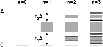
FIG. 1.: The two-scale energy spectrum. Shown are the first hierarchies in the construction of a $(r_{1},r_{2})$ fractal spectrum. The initial pattern ($n=0$) was chosen as a set of two levels, $\{\epsilon_{1}^{(0)},\epsilon_{2}^{(0)}\}=\{0,\Delta\}$. At generation $n$, $2^{n-1}$ new gaps (in gray) appear. The (positive) scale factors are restricted by the condition $r_{1}+r_{2}\leq 1$.

A very useful tool in describing Boltzmann systems with fractal spectra[8, 9] is the integrated density of states ${\cal N}(\epsilon)$ defined as

$${\cal N}(\epsilon)\equiv\int_{0}^{\epsilon}{\rm d}\epsilon^{\prime}D(\epsilon^{\prime})~{},$$ (1)

where $D(\epsilon)$ is the one-particle state density. In spite of the very fragmented structure of the density of states (a set of delta functions with fractal support), a smooth approximation is usually good enough for computing integral quantities, e.g., the specific heat. In the present case, the scaling properties of the spectrum imply that in a log-log plot ${\cal N(\epsilon)}$ looks as a self-similar staircase with a fractional average slope. If first-order log-periodic corrections are included, we obtain a smooth approximation of the form[9]

$${\cal N}(\epsilon)/2^{n+1}\approx\epsilon^{d}[a\,+\,b\cos(\omega\ln\epsilon-\phi)]~{}.$$ (2)

The so-called spectral dimension $d$[11] and the frequency $\omega$ arise from simple scaling arguments, yielding

$$d=-\ln 2/\ln r_{1}~{}~{};~{}~{}\omega=-2\pi/\ln r_{1}~{}.$$ (3)

The parameters $a\approx 1$, $b$, and $\phi$ are functions of both $r_{1}$ and $r_{2}$ and result from a detailed analysis of the exact spectral staircase. The smooth cummulative density (2) allows for analytical manipulations while still keeping the principal ingredients of the self-similar spectrum. In fact, in the Boltzmann case, the use of (2) together with a perturbative approach leads to an accurate expression for the specific heat per particle as a function of the temperature $T$:

$$c(T)\approx d+a^{\prime}\cos(\omega\ln T-\phi)~{},$$ (4)

where $a^{\prime}\ll d$ is a function of $r_{1}$ and $r_{2}$[9]. Eq. (4) relates explicitly the log-periodic nature of the specific heat to that of the spectral staircase.

III Phonon statistics

A standard way to study the acoustic properties of a lattice is to consider a nearest-neighbor harmonic chain. This model is represented by the equation of motion

$$m_{j}\frac{d^{2}u_{j}}{dt^{2}} = k_{j,j+1}u_{j+1}+k_{j,j-1}u_{j-1}$$ (6)

$$-(k_{j,j+1}+k_{j,j-1})u_{j}~{},$$

where $u_{j}$ is the displacement of the $j$th atom (of mass $m_{j}$) from its equilibrium position. $k_{j,j\pm 1}$ are the strengths of the couplings between neighboring atoms. Deterministic disorder is introduced by requiring the masses and/or the strengths to follow substitutional (e.g., Thue-Morse, Fibonacci, Fibonacci-class[12]) or hierarchical sequences. Assuming that the time dependence in (6) goes like $u_{j}\propto\exp(-i\omega t)$, the stationary equation of motion is obtained. Upon diagonalization one calculates the normal modes and the eigenfrequencies $\omega$. In the case of Thue-Morse[6], Fibonacci[13, 14, 15, 16] and Fibonacci-class[17] sequences the spectrum of energies $\epsilon=\hbar\omega$ has a Cantor-like structure only in the short wavelength regime. For long wavelengths the number of gaps and their sizes tend to zero and one recovers the standard results for the periodic lattices. On the other side, the hierarchical chains of Refs. [4, 5] do possess spectra with uniform scaling of the type ($r_{1},r_{2}$). For these cases we can apply the formalism of [9] to obtain an explicit expression for the specific heat. The specific heat per atom $c(T)$ is calculated as

$$c(T)=\frac{1}{2^{n+1}}\sum_{j=1}^{2^{n+1}}\left[\frac{\epsilon_{j}/2T}{\sinh(\epsilon_{j}/2T)}\right]^{2}~{},$$ (7)

where the summation runs over all energy levels of a ($r_{1},r_{2}$) fractal of $n$-th generation. In Fig. 2 we illustrate the dependence of the specific heat (7) with temperature for different values of $(r_{1},r_{2})$. Logarithmic scales have been used to clearly display that, in the low temperature regime ($T\ll 1$), a) $c(T)$ increases in average as power law; b) there are log-periodic corrections to the average power law. As $T$ is lowered this behavior persists down to a minimum temperature $T_{min}\approx r_{1}^{n}$, corresponding to the smallest scale of the fractal truncated at hierarchy $n$ (when $n\rightarrow\infty$, $T_{min}\rightarrow 0$). Of course, for high temperatures ($T\gg 1$), the classical result $c(T)=1$ for a one dimensional lattice is recovered. Features a) and b) can be shown to be a direct consequence of the log-periodicity of the spectral staircase, which is captured by the smooth approximation (2). In order to show that this is the case let us first rewrite (7) as an integral:

$$c(T)=\frac{1}{2^{n+1}}\int_{0}^{1}\left[\frac{\epsilon/2T}{\sinh(\epsilon/2T)}\right]^{2}d{\cal N}(\epsilon)~{}.$$ (8)

Now we make two approximations in Eq. (8). First we replace the exact ${\cal N}(\epsilon)$ by its smooth version (2). Second: as our interest is the low-$T$ regime, we extend the upper integration limit to infinity (this is equivalent to considering an unbounded fractal spectrum). After some simple algebra we arrive at

$$c(T) \approx T^{d}\,d\,[a^{\prime\prime}+b^{\prime\prime}\cos(\omega\ln T-\phi)+$$ (10)

$$c^{\prime\prime}\sin(\omega\ln T-\phi)]~{}.$$

Here $a^{\prime\prime}=aa^{\prime}$, $b^{\prime\prime}=b\,(b^{\prime}-c^{\prime}\omega/d)$, and $c^{\prime\prime}=-b\,(c^{\prime}+b^{\prime}\omega/d)$; the parameters $a^{\prime}$, $b^{\prime}$, $c^{\prime}$ are given by

$$\left[\matrix{a^{\prime}\cr b^{\prime}\cr c^{\prime}\cr}\right]=\frac{1}{4}\int_{0}^{\infty}dx\,\frac{x^{d+1}}{\sinh^{2}(x/2)}\left[\matrix{1\cr\cos(w\ln x)\cr\sin(w\ln x)\cr}\right].$$ (11)

Eq. (10) is the phonon analogue of the Boltzmann result (4). It displays explicitly the average behavior of the specific heat and the log-periodic corrections. In Fig. 2 we have plotted the analytical curves (10) for the same set of scaling factors used for the numerically exact calculations.

FIG. 2.: Phonons in a two-scale fractal spectrum. (a) Log-log plot of the specific heat per atom versus temperature. The curves are parametrized by the scale factors $(r_{1},r_{2})$ indicated in the figure. (b) $c(T)/T^{d}$ vs $\ln T$. In all cases $n=9$. Full lines correspond to numerical results (7) and dotted ones to our analytical prediction (10), which is valid only for low temperatures (this is the reason why the analytical curves do not saturate at high temperatures).

For low temperatures, the agreement between the exact and analytical results is very good [notice that the disagreement in the mean value for the $(0.30,0.15)$ case actually corresponds to a $3\%$ error]. The scale factor $r_{1}$ is responsible for the period of the oscillations through $\omega=-2\pi/\ln r_{1}$ (as shown in Fig. 2b the period decreases as $r_{1}$ increases). Moreover, as $r_{1}$ controls the gap-scaling with respect to $T=0$, smaller $r_{1}$ values imply comparatively bigger gaps, and, in turn, bigger amplitudes. For fixed $T$, decreasing $r_{1}$ causes the spectrum to shrink towards $\epsilon=0$, as a consequence the specific heat grows. These are the features observed by Petri and Ruocco in their paper on one dimensional chains with hierarchical couplings[4]. We can now understand quantitatively their results as being a direct consequence of log-periodic corrections to the pure power-law scaling of the density of states (2).

IV Bose and Fermi statistics

The statistical problem of particles with non identically null chemical potential stands at the next level of complexity, both from analytical and numerical points of views. As in this case analytical derivations seem not feasible (except in limiting regimes), we resort to a numerical procedure. For a fixed average number of particles $N$ we extracted the chemical potential $\mu$ as a function of the temperature by solving the equation

$$N=\sum_{j=1}^{2^{n+1}}\frac{1}{e^{(\epsilon_{j}-\mu)/T}\pm 1}~{},$$ (12)

where the sum runs over the levels of the fractal truncated at hierarchical depth $n$. The sign $+/-$ corresponds to the Fermi/Bose case. (We are not taking into account spin degeneracies, which will not modify our results.) The numerical solution of Eq. (12) is not a difficult task, however some care has to be taken with the choice of an appropriate initial value for $\mu$. Once the chemical potential has been obtained, the specific heat can be calculated as the $T$-derivative of the average total energy $E(T)$,

$$E(T)=\sum_{j=1}^{2^{n+1}}\frac{\epsilon_{j}}{e^{(\epsilon_{j}-\mu)/T}\pm 1}~{}.$$ (13)

A Bosons

Even though bosonic excitations with non-null chemical potential do not seem to be of main relevance for the thermodynamics of superlattices, we decided to include a discussion on this topic for reasons of completeness, and because bosons in a fractal spectrum display a paradigmatic behavior.

The dependence of the fugacity $z=\exp(\mu/T)$ with temperature is illustrated in Fig. 3a. Several curves, parametrized by the average particle number (indicated in the figure) have been drawn. First of all, Fig. 3a displays the following limiting features. As $T$ decreases, and the system evolves towards condensation, the chemical potential increases from negative values up to a limiting value close to zero (we recall that our lowest energy is $\epsilon=0$). The number of particles in the condensate is given by $N_{0}=z/(1-z)$. Thus, for very low $T$, together with large $N$, one has $z\approx 1-1/N$. In the opposite limit of high temperatures and small $N$, one obtains from (12) $z\rightarrow N^{*}\equiv N/2^{n+1}$. In Fig. 3b we have chosen a small value of $r_{1}$ to show that $\mu$ indeed oscillates as the temperature gets through the scales of the spectrum. In this sense, Fig. 3b can be thought as an amplified version of Fig. 3a.

FIG. 3.: Bosons in a two-scale fractal spectrum. Fugacity $z$ vs. $\ln T$, for different values of particle number $N$ (indicated in the figure). The chosen scales are $(r_{1},r_{2})=(1/3,0.2)$ in (a) and $(0.02,0.2)$ in (b). In both cases $n=7$.

The dependence of the specific heat per particle on the temperature is illustrated in Fig. 4. Shown are the exact result and the numerical calculation which uses the smooth expression (2) for the spectral staircase. For low temperatures the agreement is excellent. It is clear that the mean value of the specific heat is indeed associated to the average level density and that it suffices to take into account only the first non-trivial correction to the power-law scaling to explain the oscillations. [It is worth pointing out that this scenario breaks down in the fermionic case (see later)]. We have tested that the curves in Fig. 4 do not change in the thermodynamical limit of increasing both $N$ and the hierarchy $n$ but keeping $N^{*}=N/2^{n+1}$ fixed, except that the oscillatory behavior extends to lower temperatures of the order of $r_{1}^{n}$ (the total number of oscillations of the specific heat is equal to the depth $n$). The relative particle number $N^{*}$ plays the role of a density, given that the number of levels below a certain energy grows with the volume of the system. When $N^{*}$ is sufficiently small and the temperature is high enough, the curves tend to those for the Boltzmann statistics[8, 9]. This is analogous to the usual statement that the parameter $\lambda^{3}\rho$ (where $\lambda$ and $\rho$ are the thermal length and the density, respectively) tells how good is the classical approximation.

FIG. 4.: Bosons in a two-scale fractal spectrum. Log-log plot of the exact specific heat per particle $c(T)$ vs. $T$, for different values of average particle number $N$ (full lines). Dotted lines represent a calculation which uses the cummulative density of states (2). The horizontal line is $c(T)=d$, which is the classical average value for low $T$. At high temperature, the specific heat decays according to the classical $1/T^{2}$ law. Scale factors are $(r_{1},r_{2})=(1/5,1/3)$. The fractal has depth $n=9$. Base-5 logarithms were used to show that there is one oscillation per “decade”.

Although an analytical description of the problem is lacking, our numerical calculations show that log-periodicity is robust enough to resist the inclusion of bosonic symmetries together with the restriction of particle conservation.

B Fermions

The results presented in this section are valid for fermions in general, however, we assume that the fractal $(r_{1},r_{2})$ corresponds to the electronic spectrum of a certain superlattice. From the theoretical point of view, such spectra appear in the simplest model for studying the electronic properties of a lattice, i.e., a stationary tight-binding equation, for instance, in its transfer version:

$$t_{j+1}\psi_{j+1}+t_{j}\psi_{j-1}=\epsilon\psi_{j}~{},$$ (14)

where $\psi_{j}$ denotes the wave function at site $j$ and $\{t_{j}\}$ are the hopping matrix elements. If these hopping elements are arranged according to the Fibonacci sequence, the spectrum of energies $\{\epsilon\}$ is essentially a fractal of the type $(r_{1},r_{2})$ (see e.g. [7]), independently of the boundary conditions. However, the simple scaling is lost if the more general Fibonacci-class[12] sequences are considered.

The numerical scheme used for computing the thermodynamical quantities in the bosonic case can be easily adapted to the electronic problem. Figs. 5 and 6 exhibit some relations among chemical potential $\mu$, average number of particles $N$ and temperature for the $r_{1}=r_{2}=1/3$ case. Fingerprints of the fractal spectrum are clearly seen in the dependence of $\mu$ with temperature (Fig. 5). In the limit of zero temperature, for a given integer particle number $N$, $\mu$ takes the value corresponding to the middle of the gap $(\epsilon_{N},\epsilon_{N+1})$, as happens, e.g., in intrinsic semiconductors. In order to keep $N$ fixed as temperature grows, the Fermi surface moves in the direction of the lowest density of levels, integrated over an energy interval $T$. The relative concentration of levels in the neighborhood of the gap is a fluctuating function of the scale $k_{B}T$. This gives rise to an oscillatory process that persists until $T$ overcomes the largest gap ($\log_{3}T\approx-1$). From this point on, if $N^{*}>0.5$ ($N^{*}<0.5$), $\mu$ tends in a monotonic way to $+\infty$ ($-\infty$).

FIG. 5.: Fermions in a fractal spectrum. Chemical potential $\mu$ as a function of $\log_{3}T$ for all integer particle numbers $1\leq N\leq 2^{n+1}=128$ (increasing from bottom to top). We have only plotted the lower part of the full figure because it is symmetric with respect to $\mu=0.5$. Parameters are $r_{1}=r_{2}=1/3$, $n=6$.

For smaller values of $r_{1}$, oscillations in $\mu$ are magnified (not shown), analogously to what happens with bosons.

Fig. 6 displays the chemical potential as a function of the reduced number of particles $N^{*}$ for three values of fixed temperature. This figure gives some insight of the difficulties involved in solving Eq. (12). For low (fixed) temperatures, $\mu(N)$ tends to the spectral staircase and the numerical problem gets relatively difficult. As temperature grows the staircase gets smoother and numerics simplify. We have taken $N$ to be continuous, but observe that for integer $N$ and low temperatures (compared to the gap size) the curves pass through the middle of the gaps, as it is clear in Fig. 5.

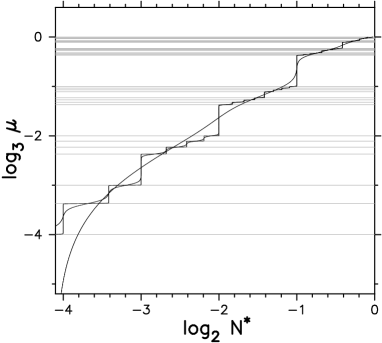
FIG. 6.: Fermions in a fractal spectrum. Log-log plot of the chemical potential $\mu$ versus the reduced number of particles $N^{*}$ for fixed temperature. The curves correspond to $T=3^{-9}$, $3^{-6}$, and $3^{-3}$ (smoother curves correspond to higher temperature). Gray lines indicate the energy levels. We used $r_{1}=r_{2}=1/3$ and $n=4$.

The specific heat in the fermionic problem depends strongly on the position of the Fermi surface. Thus, we begin by analyzing some simple cases where the number of particles takes special values. For this purpose it is useful to recall the picture of bands and gaps of Fig. 1. Each gap determines a special number of particles $N^{*}$, namely, the relative number of particles that would lie below that gap at $T=0$. For instance, the first-generation gap determines $N^{*}=1/2$. The $n=2$ gaps correspond with $N^{*}=1/4,3/4$. Conversely, the denominator and the numerator in $N^{*}$ indicate respectively the generation $n$ of a gap and the number of filled bands of $n$th generation, e.g., $N^{*}=1/32=1/2^{5}$ corresponds to a gap which appeared in the fifth generation and to one filled band of fifth generation.

A first example that illustrates the structure of the specific heat is depicted in Fig. 7. There we consider a spectrum with two different scales $r_{1}=1/3$, $r_{2}=1/9$, and the selected set of numbers $N^{*}=1/32,1/16,15/16,31/32$. For the first two cases, $N^{*}=1/32,1/16$, the size of the gap is of the order of the Fermi temperature $T_{F}$. Once the temperature overcomes the width of that gap, the electrons can fully access the next band above, so that the mean level occupation drops approximately to 1/2. From then on the electrons behave essentially as Boltzmann particles: the specific heat oscillates around a constant average value, as expressed by Eq. (4). The average value and the period are governed by the scaling factor $r_{1}=1/3$ through Eq. (3). The number of oscillations is equal to the generation index $n$: four if $N^{*}=1/16$ and five if $N^{*}=1/32$. The case of numbers $N^{*}=31/32,15/16$ is equivalent to having respectively $N^{*}=1/32,1/16$ holes and it is then complementary to the previous one. Remarkably, in the case of holes, the dominant scale is $r_{2}$. The reason for this is that $r_{2}$ rules the scaling with respect to the upper edge of the spectrum, and, in fact, with respect to the upper (lower) edge of every band (gap); in other words, $r_{2}$ is the relevant factor for negative temperatures. Eqs. (3) and (4) are still valid provided that $r_{1}$ and $r_{2}$ are interchanged. According to these arguments, the choice $r_{2}=r_{1}^{2}$ implies that the period of the oscillations for holes is twice that for electrons, which is confirmed by our calculations (see Fig. 7). Horizontal lines correspond to the Boltzmann average result, properly normalized in the case of holes. Increasing the hierarchy $n$ and keeping $N^{*}$ fixed does not change Fig. 7 because the gap on top of the filled band determines the smallest scale of the fractal that can be resolved.

FIG. 7.: Fermions in a fractal spectrum. Log-log plot of the specific heat versus temperature. The reduced numbers of particles are $N^{*}=1/32,1/16,15/16,31/32$, and the scale factors $r_{1}=1/3$, $r_{2}=1/9$. The horizontal lines represent the classical average value for the appropriate number of “hot” electrons ($N^{*}=1/32,1/16$) or holes ($N^{*}=15/16,31/32$).

Other special particle numbers allow for observing a mixed electron-hole behavior. Let us consider, for instance, the cases $N^{*}=7/64,57/64$, corresponding, respectively, to 7 and 57 filled bands of sixth generation (Fig. 8). For $N^{*}=7/64$, the Fermi temperature is several scales bigger than the width of the seventh gap, so that the low-$T$ part of the specific heat is associated to hole excitations jumping from the (empty) eighth band down over the sixth-, fifth-, and fourth-generation gaps. These excitations are of Boltzmann nature and govern the specific heat until the temperature becomes of the order of $T_{F}$. At this point electrons are able to jump up over the third-generation gap between the eighth and ninth bands. The high-$T$ ($T>3^{-4}$) oscillations are associated to electronic excitations through the third-, second-, and first-generation gaps. Similar considerations apply to the complementary case $N^{*}=57/64$. The horizontal lines in Fig. 8 correspond to our predictions for the average specific heat, which take into account the effective number of electrons or holes that contribute to the specific heat in each regime. (The fact that the case $N^{*}=7/64$ presents one less oscillation than its complementary is due to an overlap of temperature scales in the transition from hole to electron behavior.)

FIG. 8.: Analogous to Fig. 7 but for the particle numbers $N^{*}=7/64,57/64$ (see text).

The general case of an arbitrary number of particles shows a non-trivial mixture of the simple behaviors described before. However, the gross features of the specific heat for arbitrary $N$ can be qualitatively (and sometimes quantitatively) understood as being a reflection of sequences of electronic and hole excitations that alternate themselves in producing the oscillatory patterns shown in Fig. 9.

FIG. 9.: Fermions in a fractal spectrum. Log-log plot of the specific heat versus temperature for the numbers $N=25,77$, and the scale factors $r_{1}=1/3$, $r_{2}=1/9$ ($n=7$).

Formulations based on smooth approximations to the density of states, analogous to those made for bosons, are bound to fail in the fermionic case. The intrinsic discontinuity of the Fermi problem, which is critically enhanced by the dual scaling respect to the lower and upper edges of the gaps, is in essence non compatible with smooth approximations (with the exception of too special cases).

V Concluding remarks

We have analyzed the quantum statistics of model systems exhibiting two-scale fractal spectra, with special emphasis on the structure of the specific heat. Our findings extend previous results on classical statistics to show that the thermodynamical manifestations of spectral fractality are robust with respect to the inclusion of quantum symmetries. The general scenario for Boltzmann and bosonic particles can be summarized as follows. In spite of the very fragmented structure of the real density of states, a formulation which starts from a smooth approximation but takes into account the coarsest log-periodic fluctuations is sufficient for a good description of the specific heat and other averaged quantities. In the case of fermions, even if a treatment which is uniform in the particle number is not possible, many features of the problem can be understood with the help of the simple results for the Boltzmann case.

Our analysis was limited to two-scale fractals. Previous results[9] indicate that provided the scaling towards the inferior limit of the spectrum is uniform, the inclusion of additional scales will not change our conclusions in what concerns the bosonic case. Fermions, however, can feel the scaling with respect to any point of the spectrum. So, the complexity of the fermionic problem would be proportional to the number of relevant scales, in spite of uniform zero-energy scaling.

Let us finish by mentioning that the log-periodicities described in this paper may be observable in real physical systems, e.g. in the Fibonacci superlattices[2, 18]. In fact, although our discussion was restricted to perfect deterministic systems, both experiments and numerical simulations by Todd et al.[18] indicate that the hierarchical organization of the electronic bands may be preserved even if substantial amounts of (random) disorder are added to the system. From a more general point of view, Saleur and Sornette[19] have demonstrated that the connection between discrete scale invariance and log-periodic oscillations is robust with respect to the presence of disorder.

- [1] D. Schechtman, I. Blech, D. Gratias and J. W. Cahn, Phys. Rev. Lett. 53, 1951 (1984).
- [2] R. Merlin, K. Bajema, R. Clarke, F.-Y. Juang and P. K. Bhattacharya, Phys. Rev. Lett. 55, 1768 (1985).
- [3] Z. Cheng, R. Savit and R. Merlin, Phys. Rev. B 37, 4375 (1988).
- [4] A. Petri and G. Ruocco, Phys. Rev. B 51, 11399 (1995).
- [5] J. C. Kimball and H. L. Frisch, J. Stat. Phys. 89, 453 (1997).
- [6] F. Axel and J. Peyrière, J. Stat. Phys. 57, 1013 (1989).
- [7] Q. Niu and F. Nori, Phys. Rev. Lett. 57, 2057 (1986).
- [8] C. Tsallis, L. R. da Silva, R. S. Mendes, R. O Vallejos and A. Mariz, Phys. Rev. E 56, R4922 (1997).
- [9] R. O. Vallejos, R. S. Mendes, L. R. da Silva and C. Tsallis (preprint cond-mat/9803265).
- [10] See e.g. T. Tél, Z. Naturforsch. 43a, 1154 (1988).
- [11] S. Alexander and R. Orbach, J. Physique Lett. 43, L-625 (1982); R. Rammal and G. Toulouse, J. Physique Lett. 44, L-13 (1983); C. Tsallis and R. Maynard, Phys. Lett. A 129, 118 (1988).
- [12] X. Fu, Y. Liu, P. Zhou and W. Sritrakool, Phys. Rev. B 55, 2882 (1997).
- [13] J. M. Luck and D. Petritis, J. Stat. Phys. 42, 289 (1986).
- [14] F. Nori and J. P. Rodriguez, Phys. Rev. B 34, 2207 (1986).
- [15] J. P. Lu, T. Odagaki, and J. L. Birman, Phys. Rev. B 33, 4809 (1986).
- [16] Y. Liu and R. Riklund, Phys. Rev. B 35, 6034 (1987).
- [17] C. Anteneodo and R. O. Vallejos (unpublished).
- [18] J. Todd, R. Merlin, R. Clarke, K. M. Mohanty, and J. D. Axe, Phys. Rev. Lett. 57, 1157 (1986).
- [19] H. Saleur and D. Sornette, J. Phys. I France 6, 327 (1996).