Interfaces and Grain Boundaries of Lamellar Phases

Abstract

Interfaces between lamellar and disordered phases, and grain boundaries within lamellar phases, are investigated employing a simple Landau free energy functional. The former are examined using analytic, approximate methods in the weak segregation limit, leading to density profiles which can extend over many wavelengths of the lamellar phase. The latter are studied numerically and exactly. We find a change from smooth chevron configurations typical of small tilt angles to distorted omega configurations at large tilt angles in agreement with experiment.

, , and

1 Introduction

Lamellar phases are found in many systems, such as ferrofluids, mixtures of lipids and water, and melts of diblock copolymers [1]. Whenever such phases occur, one expects to observe grain boundaries between phases of different orientations. While such boundaries have been the subject of much study in solids, there has been very little work on their occurrence in complex fluids. The recent experimental work of Gido and Thomas [2] and Hashimoto et al. [3] on grain boundaries in diblock copolymer systems showed that the conformation of the boundary was a strong function of the angle between grains. Whereas for small angles, the lamellae varied smoothly from one orientation to the other, (a “chevron” configuration), for larger angles the lamellae became quite distorted, sending out a piece of lamellae nearly parallel to the boundary itself (an “omega” configuration). Finally, when the interface is parallel to the lamellae of one of the two adjoining phases, the lamellae became disjunct, abutting one another in a “T-junction”. In this paper, a simple Landau free energy is shown to produce precisely this behavior.

In addition, we consider the interface between coexisting lamellar and disordered phases. Again such interfaces occur in many systems: those of pure diblock copolymer melts [4], of mixtures of homopolymer and diblock [5], of lipids and water [6], of small amphiphiles, oil and water [7] etc. The interface is studied analytically in the weak-segregation limit i.e. in which the ordering of the lamellae can be described by a single Fourier amplitude.

2 The Model

We consider a three-dimensional system in which the ordering can be described by a scalar order parameter $\phi$, and employ the dimensionless Ginzburg-Landau free energy functional (rescaled by $k_{B}T$)

$${F}[\phi] = \int\left\{-\frac{\chi}{2}\phi^{2}+\frac{1}{2}(\nabla^{2}\phi)^{2}-\frac{1}{2}(\nabla\phi)^{2}\right.$$ (1)

$$\left.+~{}~{}\frac{1-\phi}{2}\ln\frac{1-\phi}{2}+\frac{1+\phi}{2}\ln\frac{1+\phi}{2}\right\}{\rm d}V$$

The interaction term, of strength $\chi$, induces the system to order ($\phi\neq 0$) as $\chi$ increases. That the coefficient of the gradient squared term is negative expresses the system tendency to make this ordered phase a modulated one in which the order parameter varies in space. The positive coefficient of the Laplacian squared term ensures that the spatial variation does not become too large. Finally, the logarithmic entropy of mixing terms oppose the tendency to order, preferring a state in which $\phi$ vanishes. Note that the order parameter $\phi$ is limited to have magnitude less than or equal to unity. The coefficients of the Laplacian squared and gradient squared terms are chosen to be $\pm 1/2$, respectively, setting the length scale in the problem. For convenience, we first turn to the weak segregation limit and the interface between lamellar and disordered phases.

3 The Lamellar-Disorder Interface in Weak Segregation

We assume here that the ordering is weak, i.e. that $|\phi|$ is small. In that case the free energy functional can be expanded to fourth order in $\phi$. We restrict ourselves to lamellar phases, and introduce the Fourier representation $\phi(x)=\sum\phi_{k}\exp(i{k}{x})$, with $\phi_{k}=\phi_{-k}^{*}$ as the order parameter is real. In this representation the free energy per unit volume is

$$\frac{{F}}{V}=\frac{1}{2}\sum_{k}A_{k}\phi_{k}\phi_{-k}+\frac{1}{12}\sum_{k,p,q}\phi_{k}\phi_{p}\phi_{q}\phi_{-(k+p+q)}$$ (2)

where a non relevant constant term is omitted from $F$, and $A_{k}\equiv[1-\chi-k^{2}+k^{4}]$. The $k$-mode which becomes critical at the highest temperature is that for which $A_{k}$ is minimal. This occurs at $k=1/\sqrt{2}\equiv q$, at which $A_{q}=3/4-\chi$. When $\phi_{q}$ is small, all other $\phi_{k}$, save $\phi_{0}$, can be ignored as they are proportional to integer powers of $\phi_{q}$. Hence

$$\frac{{F}}{V}\approx\frac{1}{2}(1-\chi)\phi_{0}^{2}+\frac{1}{12}\phi_{0}^{4}+\left(\frac{3}{4}-\chi+\phi_{0}^{2}\right)\phi_{q}\phi_{-q}+\frac{1}{2}(\phi_{q}\phi_{-q})^{2}.$$ (3)

Minimizing this free energy with respect to $\phi_{q}\phi_{-q}=|\phi_{q}|^{2}$, one obtains

$$\phi_{q}\phi_{-q}|_{min}=(\chi-\phi_{0}^{2}-3/4).$$ (4)

As this must be positive, it follows that in the lamellar phase, $0\leq\phi_{0}^{2}\leq\chi-3/4$. A line of continuous transitions from the disordered to lamellar phase occurs when $\phi_{q}$ vanishes, i.e. along the line

$$\chi_{c}=\phi_{0}^{2}+3/4.$$ (5)

Upon substitution of the minimum value of the order parameter, Eq. (4), into the free energy of Eq. (3), one finds that in the lamellar phase,

$$\frac{{F}^{L}(\phi_{0},\chi)}{V}=-\frac{1}{2}\left(\frac{3}{4}-\chi\right)^{2}+\frac{1}{2}\left(\chi-\frac{1}{2}\right)\phi_{0}^{2}-\frac{5}{12}\phi_{0}^{4},$$ (6)

as compared to the free energy of the disordered phase which, from Eq. (3) with $\phi_{q}=0$, is

$$\frac{{F}^{D}(\phi_{0},\chi)}{V}=\frac{1}{2}(1-\chi)\phi_{0}^{2}+\frac{1}{12}\phi_{0}^{4}.$$ (7)

The line of continuous transitions ends at a tricritical point at which the free energy of the lamellar phase, Eq. (6), is no longer convex with respect to $\phi_{0}$. This occurs at the point $\phi_{0}^{t}=1/4$, and $\chi^{t}=13/16$. For larger values of $\chi$ and $\phi_{0}$, the system undergoes phase separation, with lamellar and disordered phases coexisting. The value of $\phi_{0}$ in each, denoted $\phi_{0}^{L}$ and $\phi_{0}^{D}$, respectively, is obtained from the conditions of the equality of chemical potentials, $\mu$,

$$\frac{1}{V}\frac{\partial{F}^{L}(\phi_{0}^{L},\chi)}{\partial\phi_{0}^{L}}=\frac{1}{V}\frac{\partial{F}^{D}(\phi_{0}^{D},\chi)}{\partial\phi_{0}^{D}}$$ (8)

and of grand potentials $G/V\equiv F/V-\mu\phi_{0}$

$$F^{L}(\phi_{0}^{L},\chi)-\frac{\partial{F}^{L}(\phi_{0}^{L},\chi)}{\partial\phi_{0}^{L}}\phi_{0}^{L}=F^{D}(\phi_{0}^{D},\chi)-\frac{\partial{F}^{D}(\phi_{0}^{D},\chi)}{\partial\phi_{0}^{D}}\phi_{0}^{D}.$$ (9)

Once $\phi_{0}^{L}$ is known, the amplitude of the modulation in the coexisting lamellar phase follows from Eq. (4). We now turn to the calculation of the interfacial profile, $\phi(x)$, between these phases.

The interfacial free energy per unit area (and in units of $k_{B}T$) is the minimum of the functional

$$\sigma[\phi]=\int{\rm d}x\left\{\frac{1}{V}F[\phi]-\mu\phi(x)-\frac{1}{2V}(G^{L}+G^{D})\right\}.$$ (10)

where the first term $F[\phi]/V$ is just the local free energy density as appearing under the spatial integration of Eq. (1), and $G^{L}$ and $G^{D}$ are the lamellar and disordered bulk grand potentials, respectively, as defined above. The Euler-Lagrange equation which results from this minimization is to be solved for the profile subject to the boundary conditions $\phi(x)\rightarrow\phi_{0}^{D}$ as $x\rightarrow\infty$, and $\phi(x)\rightarrow\phi_{0}^{L}+2|\phi_{q}|\cos(qx)$ as $x\rightarrow-\infty$. Rather than solve this equation directly, we use the ansatz $\phi(x)=\phi_{0}^{D}[1+f(x)]/2+\phi_{0}^{L}[1-f(x)]/2+g(x)|\phi_{q}|\cos(qx)$ where $f(x)$ and $g(x)$ approach 1 and 0, respectively as $x\rightarrow\infty$, and $-1$ and 2, respectively as $x\rightarrow-\infty$. Near the tricritical point, we can expand the amplitudes $\phi_{0}^{D}$, $\phi_{0}^{L}$, and $\phi_{q}$ about the values they take at the tricritical point, 1/4, 1/4, and 0, respectively, in a power series in $\chi-\chi^{t}$. Solving the equations for $f(x)$ and $g(x)$ to lowest order in this small parameter, we find [8]

$$g(x)=\frac{2{\rm e}^{-U}}{\sqrt{1+{\rm e}^{-2U}}},$$ (11)

$$f(x)=\tanh(U)-\frac{18}{5\cosh^{2}(U)}(\chi-\chi^{t})$$ (12)

where $U(x)=2(3/5)^{1/2}(\chi-\chi^{t})x.$ A profile for the case $\chi=0.9$ is shown in Fig. 1. Several lamellae participate in the interfacial region for this weak first order transition.

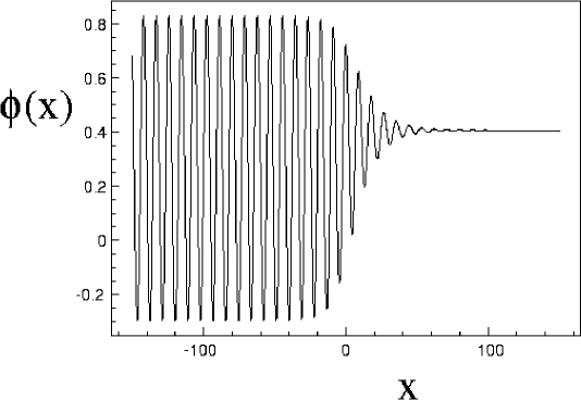
Figure 1: Interfacial profile between lamellar and disordered phases for $\chi=0.9$ (weak segregation limit).

As the tricritical point is approached, the width of the interface, governed by the bulk correlation length, $\xi$, will diverge, of course. In our calculation, we find the expected mean-field scaling [9] $\xi\sim 1/(\chi-\chi^{t})$. The wavelength characterizing the lamellar phase, however, remains at $2\pi/q$. Thus there are many oscillations of the order parameter within the interface as the tricritical point is approached. The evaluation of the interfacial tension itself proceeds in a similar manner, and one obtains the scaling $\sigma\sim(\chi-\chi^{t})^{2}$ expected within mean-field theory of tricritical points [9].

We close this section by noting that these interfacial phenomena associated with the occurrence of a tricritical point can be observed for uniaxial lamellar systems, such as thermotropic liquid crystal at the nematic/smectic-A transition [10]. If phases of hexagonal symmetry are allowed, the line of critical phase transitions between disordered and lamellar phases, which ends at the tricritical point, is pre-empted by a line of first-order phase transition between disordered and hexagonal phases. Only the continuous transition at $\phi_{0}=0$ remains. Thus, the interface we have considered close to a tricritical point exists only between metastable phases. Nonetheless, the general results we obtain should apply also to isotropic systems when there is a weak first-order transition between disordered and lamellar phases. As noted earlier, this is the case in many systems: pure diblock copolymers [4], copolymer mixtures [5], lipid and water mixtures [6], and ternary mixtures of small amphiphiles, oil and water [7]. In each case, one expects an interface in which the transition from the lamellar to the disordered phase occurs over a length scale, $\xi$, which is quite large with respect to the wavelength $\lambda$ of the lamellar phase itself. The interfacial tension between phases, $\sigma$, will be small if the first-order transition is weak.

4 Grain Boundaries in Lamellar Phases of Complex Systems

We next consider grain boundaries between lamellar phases and do so by considering the free energy of Eq. (1). In contrast to the analytic, approximate treatment above, in this section we minimize the free energy numerically, and exactly [11]. To do so, we discretize space into a 200 by 200 lattice, and minimize the free energy functional with respect to the order parameter amplitude on the 40,000 lattice sites by means of a conjugate-gradient method. Appropriate boundary conditions are imposed to bring about a grain boundary. We set the parameter $\chi$ and $\phi_{0}$ such that the lamellar phase is stable. In the results below, $\chi=1$, and $\phi_{0}=0$. Fig. 2(a) shows a symmetric tilt boundary with an angle of $28.08^{\circ}$ between the lamellae normals.

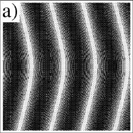
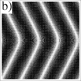
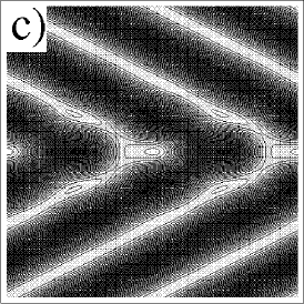
Figure 2: Order parameter profiles for symmetric tilt grain boundaries for $\phi_{0}=0$ and $\chi=1$. The order parameter ranges from $-1$ to 1, and is represented by 20 grayscales. (a) $\theta=28.08^{\circ}$; (b) $\theta=53.14^{\circ}$, (c) $\theta=126.86^{\circ}$.

The configuration is clearly that denoted “chevron” in ref. [2]. This smooth configuration remains when the tilt angle is increased, in Fig. 2(b), to $\theta=53.14^{\circ}$. However when the angle is increased to 126.86^∘, as in Fig. 2(c), the configuration has changed markedly to that denoted “omega” in ref. [2]. The change in configuration is clearly due to the fact that the spacing between lamellae at the grain boundary itself, $\lambda/\cos(\theta/2)$, is so much larger than the preferred spacing, $\lambda$. By sending out the tip observed in Fig. 2(c), the distance between regions of the same sign of the order parameter is reduced.

As the system is brought close to the transition to the disordered phase, we observe a pronounced reconstruction of the grain boundary in terms of a square-like modulation. This is shown in Fig. 3 for $\chi=0.78$.

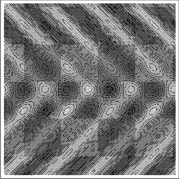
Figure 3: Symmetric tilt grain boundary with $\theta=90^{\circ}$, and $\chi=0.78.$

The symmetric tilt-boundary free energy per unit area, $\sigma_{TB}$, decreases as the transition is approached and, for $\phi_{0}=0$, vanishes as $\sigma_{TB}\sim(\chi-3/4)^{3/2}$ in accord with mean-field predictions. As the angle of the tilt-boundary approaches zero, its free energy vanishes as $\theta^{3}$; as the angle approaches $\pi$, the energy is expected to vanish linearly with $(\pi-\theta)$ in accord with a description in terms of independent dislocations of finite creation energy.

Finally we turn to the “asymmetric” T-junction. In Fig. 4, we show results for this junction, again at $\chi=1$ and $\phi_{0}=0$. In contrast to the chevron and omega configurations, only one of the two types of domains is continuous across the interface in the T-junction.

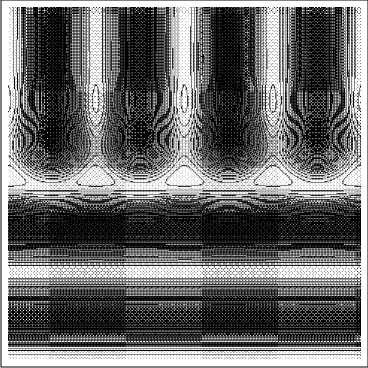
Figure 4: Asymmetric grain boundary (T-junction) between two perpendicular lamellar phases at $\phi_{0}=0$ and $\chi=1$.

Note the enlarged endcaps of the terminated lamellae, a feature which is also clearly observable in experiment. We find that these endcaps become less prominent as $\chi$ is increased. The free energy of this junction also vanishes as $(\chi-3/4)^{3/2}$ as expected in mean-field theory. More interestingly, we find that the free energy of this boundary is much less than that brought about by inserting one wavelength of disordered phase between the grains. Thus, the reconstruction at the boundary is a far more efficient way of making the transition from one orientation to another than that of a grain boundary melting.

In summary, we have employed a simple Ginzburg-Landau free energy and calculated analytically, and approximately, the properties of an interface between a lamellar phase and a disordered one in a weak segregation limit. We have used the same free energy to calculate numerically, and exactly, the form of the grain boundaries between lamellar phases. The agreement with experiment is excellent. As this has been obtained from a Landau free energy, this phenomena must result from a full mean-field calculation as well [12]. Finally, we are able to make additional predictions concerning the reconstruction of these interfaces as the temperature of the system is varied. In physical systems (block copolymers and others), phases of hexagonal and cubic symmetry are found in addition to the lamellar ones. It will be most interesting to investigate the interfaces and grain boundaries of these phases, as we have done here for the lamellar one.

We acknowledge support from the United States-Israel Binational Science Foundation under grant no. 94-00291, and the National Science Foundation under grant no. DMR 9531161. One of us (SVG) thanks the French Ministry of Foreign Affairs for a research fellowship.

References

- [1] M. Seul and D. Andelman, Science 267 (1995) 476.
- [2] S.P. Gido and E.L. Thomas, Macromolecules 27 (1994) 6137.
- [3] T. Hashimoto, S. Koizumi and H. Hasegawa, Macromolecules 27 (1994) 1562.
- [4] F.S. Bates, M.F. Schulz, A.K. Khandpur, S. Förster, and J.H. Rosedale, Faraday Discuss. 98 (1994) 7.
- [5] F.S. Bates, W. Maurer, T.P. Lodge, M.F. Schulz, M.W. Matsen, K. Almdal, and K. Mortensen, Phys. Rev. Lett. 75 (1995) 4429.
- [6] J. Briggs and M. Caffrey, Biophysical Journal 67 (1994) 1594.
- [7] R. Strey, Ber. Bunsenges. Phys. Chem. 97 (1993) 742.
- [8] S. Villain-Guillot and D. Andelman, submitted to J. de Physique (France).
- [9] J.S. Rowlinson and B. Widom, Molecular Theory of Capillarity (Oxford University Press, New York, 1982).
- [10] J.D. Litster and R.J. Birgeneau, Phys. Today 35, No. 5 (1982) 261.
- [11] R.R. Netz, D. Andelman, and M. Schick, submitted to Physical Review Letters.
- [12] That this is the case has been shown by M. Matsen, private communication.