A geometric generalization of field theory to manifolds of arbitrary dimension

Abstract

We introduce a generalization of the $O(N)$ field theory to $N$-colored membranes of arbitrary inner dimension $D$. The $O(N)$ model is obtained for $D\to 1$, while $N\to 0$ leads to self-avoiding tethered membranes (as the $O(N)$ model reduces to self-avoiding polymers). The model is studied perturbatively by a 1-loop renormalization group analysis, and exactly as $N\to\infty$. Freedom to choose the expansion point $D$, leads to precise estimates of critical exponents of the $O(N)$ model. Insights gained from this generalization include a conjecture on the nature of droplets dominating the $3d$-Ising model at criticality; and the fixed point governing the random bond Ising model.

PACS numbers: 05.70.Jk, 11.10.Gh, 64.60.Ak, 75.10.Hk

Field theories have strong connections to geometrical problems involving fluctuating lines. For example, summing over all world-lines representing the motion of particles in space-time, is the Feynman path integral approach to calculating transition probabilities, which can also be obtained from a quantum field theory. Another example is the high-temperature expansion of the Ising model, where the energy-energy correlation function is a sum over all self-avoiding closed loops which pass through two given points. Generalizing from the Ising model to $N$ component spins, the partition function of a corresponding $O(N)$ “loop model” is obtained by summing over all configurations of a gas of closed loops, where each loop comes in $N$ colors, or has a fugacity of $N$. In the limit $N\to 0$, only a single loop contributes, giving the partition function of a closed self-avoiding polymer[1].

There are several approaches to generalizing fluctuating lines to entities of other internal dimensions $D$. The most prominent examples are string theories and lattice gauge theories, which both describe $D=2$ world sheets[2]. The low temperature expansion of the Ising model in $d$ dimensions also results in a sum over surfaces that are $d-1$ dimensional. Each of these generalizations has its own strengths, and offers new insights on field theory. Here we introduce a generalization based on a class of $D$-dimensional manifolds called “tethered” (or polymerized) membranes, which have fixed internal connectivity, and are the simplest generalization of linear polymers[3].

Tethered manifolds are a quite successful generalization of self-avoiding polymers embedded in $d$-dimensional external space: Simple power counting indicates that self-avoidance is relevant only for dimensions $d<d_{c}=4D/(2-D)$, making possible an $\varepsilon=2D-d(2-D)/2\sim(d_{c}(D)-d)$-expansion, which was first carried to 1-loop order in Refs. [4]. Following more rigorous analysis of this novel perturbation series [5], recently 2-loop calculations were performed for $1\leq D<2$ [6]. To obtain results for polymers or membranes, one has the freedom to expand about any inner dimension $D$, and the corresponding upper critical dimension of the embedding space[7]. This

FIG. 1.: Schematic depiction of the model, and its limits.

freedom can be used to optimize calculation of critical exponents, and when applied to polymers, the results are clearly better than those from the standard expansion.

Our basic idea is to generalize the high temperature expansion of the $O(N)$ model, from a gas of self-avoiding loops of fugacity $N$, to a similar gas of closed fluctuating manifolds of internal dimension $D$. The primary goal is to obtain a novel analytical handle on the field theory for $D=1$, and we do not insist that the models for general $D$ correspond to any physical problem. Given this caveat, the generalization is not unique. Encouraged by its success in polymer theory, we study tethered manifolds, and in addition restrict ourselves to the genus of hyper-spheres. We have chosen hyperspheres as they have no additional anomalous correction exactly at $D=2$. The resulting manifold theory depends on two parameters $N$ and $D$, whose limiting behaviors reduce to well known models, as indicated in Fig. 1.

We construct the $M(N,D)$ manifold model perturbatively, starting with the well known high-temperature expansion (loop-model) of the $O(N)$ field theory as

$$\ln{\cal Z} = \,\!\!\!\raisebox{-7.96661pt}{ \begin{picture}(11.0,10.0)(0.0,0.0)\put(1.0,5.0){\put(0.0,0.0){\circle*{2.0}} \put(5.0,0.0){\circle{10.0}} }\end{picture}}\,+\,\!\!\!\raisebox{-7.96661pt}{ \begin{picture}(26.0,10.0)(0.0,0.0)\put(16.0,5.0){ \put(-15.0,0.0){\circle*{2.0}} \put(-5.0,0.0){\dashbox(0.5)(5.0,0.0)[]{}} \put(-5.0,0.0){\circle*{2.0}} \put(0.0,0.0){\circle*{2.0}} \put(5.0,0.0){\circle{10.0}} \put(-10.0,0.0){\circle{10.0}} }\end{picture}}\,+\,\!\!\!\raisebox{-7.96661pt}{ \begin{picture}(16.0,10.0)(0.0,0.0)\put(1.0,5.0){ \put(0.0,0.0){\circle*{2.0}} \put(7.5,5.0){\circle*{2.0}} \put(7.5,-5.0){\circle*{2.0}} \put(7.5,0.0){\oval(15.0,10.0)} \put(7.5,-5.0){\dashbox(0.5)(0.0,10.0)[]{}} }\end{picture}}\,+\cdots\ .$$ (1)

The first term in this sum is the partition function of a non-interacting polymer loop, now generalized to a $D$-dimensional manifold, fixed at the origin in $d$ dimensions

$$\!\!\!\raisebox{-7.96661pt}{ \begin{picture}(11.0,10.0)(0.0,0.0)\put(1.0,5.0){\put(0.0,0.0){\circle*{2.0}} \put(5.0,0.0){\circle{10.0}} }\end{picture}}\,=\frac{c(D)}{D}\int_{0}^{\infty}{\rm d}\Omega\,\,\Omega^{-\frac{2-D}{D}d}{\rm e}^{-t\Omega}\ .$$ (2)

The integral runs over all sizes $\Omega$, weighted by a chemical potential $t$, while the factor

$$\Omega^{-{\frac{2-D}{D}d}}\sim\left<\tilde{\delta}^{d}(r(x_{0}))\right>_{0}\ ,$$ (3)

is the probability that the membrane is attached to a given point in space[5]. The above generalization depends on a function $c(D)$, related to the relative strengths of self-avoidance between parts of the same manifold, and between different manifolds. Any choice of $c(D)$ which reproduces the polymer partition function with $c(1)=1$, is acceptable. In the remainder, we will mainly focus on $c(D)=D$, equivalent to the integral ${\rm d}\Omega$ over all scales.

Subsequent terms in Eq. (1) correct for the intersections (symbolized by a dashed line) between manifolds. Configurations involving intersections between different manifolds, or self-intersections of the same manifold (e.g., the second and third terms in the above expansion, respectively) have to be subtracted from the partition function. The contributions from these terms result in divergencies which have to be removed by renormalization (for details see Ref. [8]). The final result is the 1-loop expansion of the exponent $\nu(D,N,d)$ (for the divergence of the correlation length at a critical point), given by ($\varepsilon\equiv 2D-\frac{2-D}{2}d$)

$$\nu(D,N,d)={2-D\over 2}\times$$ (4)

$$\left[1+{\varepsilon\over 2D}{1+{c(D)}{N\over 2}\over{1\over 2-D}\Gamma\left(\frac{D}{2-D}\right)^{2}{\Gamma\left(\frac{2D}{2-D}\right)^{-1}}+1+c(D){N\over 4}}\right]\ .$$ (5)

This expression reduces to the well-known $\varepsilon$-expansion[9] around $d=4$ for lines ($D=1$), while the $N\to 0$ limit reproduces the result for self-avoiding manifolds[4].

The perturbative series can also be summed exactly in the large $N$ limit, where the ambiguity associated with $c(D)$ is removed[8], to give the exponent

$$\nu_{N\to\infty}=\frac{D}{d-{2D}/{(2-D)}}\ .$$ (6)

This generalizes the well-known result of $\nu=1/(d-2)$ for the $O(N)$ model[9].

To demonstrate the utility of this generalization, we next estimate the exponent $\nu$ in physical dimensions, by expanding about a point $(D_{0},d_{0})$ on the critical curve $\varepsilon(D_{0},d_{0})=0$. The simplest scheme is to extrapolate towards the physical theories for $D=1,2$ and $d=2,3,\cdots$, with the expansion parameters $D-D_{0}$ and $d-d_{0}$. However, this choice is not optimal (see Ref. [6]), and better results are obtained with expansion parameters $D_{c}(d)={2d}/{(4+d)}$ and $\varepsilon(D,d)=2D-d{(2-D)}/2d$. Furthermore, it is better to expand $\nu d$ or $\nu(d+2)$ rather than $\nu$. The first is an expansion of the form $\nu d=2D+a(D)\varepsilon$, about the mean-field result $\nu_{\mbox{MF}}={2D}/{d}$, also known as Gaussian variational approximation[10]. The second is a similar expansion about the Flory expression $\nu_{\mbox{Flory}}=(2+D)/(2+d)$.

             $N$ 0 1 2 3 $\nu$, our result 0.601 0.646 0.676 0.697 $\nu$, from [9] 0.589 0.631 0.676 0.713

FIG. 2.: Extrapolations for the exponent $\nu$ of the $O(N)$ model in $d=3$, using the expansion of $\nu d$ with $c(D)=D$. The dashed lines represent the best known values from Ref. [9].

After selecting one of these schemes, Eq. (4) is re-expressed in terms of the chosen expansion parameters. However, we are still free to choose the expansion point along the critical curve, which then fixes $D_{0}$. As $D_{0}$ is varied, different values for $\nu$ are obtained, as ploted in Fig. 2. The criterion for selecting a particular value from such curves is that of minimal sensitivity to the expansion point, and we thus evaluate $\nu$ at the extrema. The broadness of the extremum then provides a measure for the goodness of the result, and the expansion scheme. Although we examined several such curves, only a selection is reproduced in Fig. 2. Our results are clearly better than the standard 1-loop expansion of $\nu=1/2+{(N+2)}/[{4(N+8)]}$.

While providing good estimates for exponents of the $O(N)$ model is certainly a benefit, the generalization to $M(N,D)$ should offer insights beyond the standard field theory. Also, for the approach to be more generally applicable, we should show that similar generalizations are possible for other field theories. In the rest of this article we shall demonstrate that these goals are indeed feasible.

Our starting point was the high temperature expansion of the $O(N)$ spin model, which naturally leads to a sum over $N$-colored loops ($D=1$); motivating the later generalization to $M(N,D)$. For the Ising model ($N=1$), a different geometrical description is obtained from a low temperature expansion: Excitations to the uniform (up or down pointing) ground state are droplets of spins of opposite sign. The energy cost of each droplet is proportional to its boundary, i.e. again weighted by a Boltzmann factor ${\rm e}^{-t\Omega}$. Thus, a low temperature series for the $d$-dimensional Ising partition function is obtained by summing over closed surfaces of dimension $D=d-1$. For $d=2$, the high and low temperature series are similar, due to self-duality. For $d=3$, the low temperature description is a sum over surfaces.

FIG. 3.: Test of Eq. (7) for Ising models in $d=2.5$ and $3$. The upper curves are from the high temperature representation ($D=1$), while the lower curves are from the low temperature description ($D=d-1$). The exponent $\nu$ is estimated from the maximum of each curve, which are obtained by extrapolating $\nu d$ with $c(D)=D$, linearizing in $N$, and dividing the result by $dD$.

The non-trivial question is regarding the types of surfaces which dominate the above sum. Since there is no constraint on the internal metric, it may be appropriate to examine fluid membranes. However, there is currently no practical scheme for treating interacting fluid membranes, and the excluded volume interactions are certainly essential to the problem. It is known that configurations of a single surface for $N=0$, self-avoiding or not, are dominated by tubular shapes (spikes) which have very large entropy[11]. Such “branched polymer” configurations are very different from tethered surfaces. However, for $N\neq 0$, it may be entropically advantageous to break up a singular spike into a string of many bubbles. If so, describing the collection of bubbles by fluctuating hyper-spherical (tethered) manifolds may not be too off the mark[16]. We can test the validity of this conjecture by comparing the predictions of the dual high and low-temperature descriptions.

Singularities of the partition function are characterized by the critical exponent $\alpha(D,d,N)$, or (using hyperscaling) through $\ln{\cal Z}_{\mbox{singular}}\sim|t-t_{c}|^{\nu d/D}.$ The equality of the singularities on approaching the critical point from low or high temperature sides, leads to a putative identity

$${\nu(1,d,1)}=\frac{1}{d-1}\,\nu(d-1,d,1)\ .$$ (7)

Numerical tests of the conjecture in Eq. (7) are presented in Fig. 3. The extrapolated exponents (the maxima of the curves) from the dual expansions are in excellent agreement. Nevertheless, higher-loop calculations would be useful to check this surprising hypothesis.

The simplest extension of the $O(N)$ model breaks the rotational symmetry by inclusion of cubic anisotropy[12]. In the field theory language, cubic anisotropy is represented by a term $u\sum_{i}s_{i}^{4}$, in addition to the usual interaction of $b\sum_{ij}s_{i}^{2}s_{j}^{2}$. In the geometric prescription of high temperature expansions, the anisotropic coupling $u$ acts only between membranes of the same color, while the interaction $b$ acts irrespective of color.

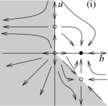
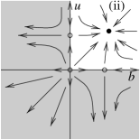
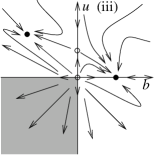
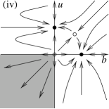
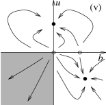
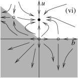
FIG. 4.: Regions with different RG-flow patterns in the $(N,D)$-plane (top), and the corresponding RG-flows (bottom); shaded regions are unstable.

Stability of the system of colored membranes places constraints on possible values of $b$ and $u$. To avoid collapse of the system, energetic considerations imply that if $u<0$, the condition $u+b>0$ must hold, while if $u>0$, we must have $u+Nb>0$[12, 8]. The above stability arguments are expected to be modified upon the inclusion of fluctuations. A well-known example is the Coleman-Weinberg mechanism [12], where the RG flows take an apparently stable combination of $b$ and $u$ into an unstable regime, indicating that fluctuations destabilize the system. In the flow diagrams described below, we also find the reverse behavior in which an apparently unstable combination of $b$ and $u$ flows to a stable fixed point. We interpret this as indicating that fluctuations stabilize the model, a reverse Coleman-Weinberg effect, which to our knowledge is new. We have shaded in grey, the unphysical regions in the flow diagrams of Fig. 4. As in their $O(N)$ counterpart, the RG equations admit 4 fixed points: The Gaussian fixed point with $b^{*}_{G}=u^{*}_{G}=0$; the Heisenberg fixed point located at $b^{*}_{H}\neq 0$, $u^{*}_{H}=0$; the Ising fixed point with $b^{*}_{I}=0$, $u^{*}_{I}\neq 0$; and the cubic fixed point at $b^{*}_{c}\neq 0$, $u^{*}_{c}\neq 0$. Furthermore, as depicted in Fig. 4, there are six different possible flow patterns. In the $O(N)$ model, the flows in (i) and (ii) occur for $N<4$ and $N>4$, respectively. The other four patterns do not appear in the standard field theory, as is apparent from their domain of applicability in the $(N,D)$ plane on Fig. 4. Note that there are two stable fixed points in three out of these four cases.

FIG. 5.: Extrapolations of $\nu$ from the expansion of $\nu d$ with $c(D)=D$, for the $O(N)$ model in $d=3$. Exponents at the Heisenberg fixed point for $N=0$ are compared to those of the Ising and cubic fixed points. The crossing of the latter curves yields an estimate of $\nu=0.6315$ for the $3d$ Ising model.

The $N\to 0$ limit of the above models is interesting, not only because of its relevance to self-avoiding polymers and membranes, but also for its relation to the Ising model with bond disorder. The latter connection can be shown by starting with the field theory description of the random bond Ising model, replicating it $N$ times, and averaging over disorder [13]. The replicated system is controlled by a Hamiltonian with positive cubic anisotropy $u$, but negative $b=-\sigma$ ($\sigma$ is related to the variance of bond disorder). From the “Harris criterion”[14], new critical behavior is expected for the random bond Ising system. But in the usual field theory treatments[13], there is no fixed point at the 1-loop order. In our generalized model, this is just the borderline between cases (i) and (iii). However, we now have the option of searching for a stable fixed point by expanding about any $D\neq 1$. Indeed, for $N=0$ and $1<D<1.29$, the cubic fixed point lies in the upper left sector ($u>0$ and $b<0$) and is completely stable, as in flow pattern (iii).

The extrapolation for $\nu$ at the cubic fixed point is plotted in Fig. 5, where it is compared to the results for the Heisenberg and Ising fixed points. The divergence of $\nu$ on approaching $D=1$ from above, is due to the cubic fixed point going to infinity as mentioned earlier. Upon increasing $D$, the Ising and cubic fixed points approach, and merge for $D=1.29$. For larger values of $D$, the cubic fixed point is to the right of the Ising one ($b_{c}^{*}>0$), and only the latter is stable. Given this structure, there is no plateau for a numerical estimate of the random bond exponent $\nu_{\mbox{DO}}$, and we can only posit the inequality $\nu_{\mbox{DO}}>\nu_{\mbox{Ising}}$. While this is derived at 1-loop order, it should also hold at higher orders since it merely depends on the general structure of the RG flows. One may compare this to four loop calculations of the random bond Ising model [15], which are consistent with $\alpha=0$, i.e. at the border-line of the Harris criterion[14], with $\nu=2/3$.

It is a pleasure to thank F. David, H.W. Diehl, and L. Schäfer for useful discussions. Part of this work was done during a visit of K.J.W. to MIT, with the financial support of Deutsche Forschungsgemeinschaft, through the Leibniz-Programm. The work at MIT is supported by the NSF Grant No. DMR-93-03667.

REFERENCES

- [1] P.-G. de Gennes, Phys. Lett. A 38, 339 (1972).
- [2] Fluctuating Geometries in Statistical Mechanics and Field Theory, F. David and P. Ginzparg, and J. Zinn-Justin, eds. (Elsevier, Amsterdam, 1996).
- [3] Y. Kantor, M. Kardar, and D. R. Nelson, Phys. Rev. Lett. 57, 791 (1986); Phys. Rev. A 35, 3056 (1987).
- [4] M. Kardar and D. R. Nelson, Phys. Rev. Lett. 58, 1289 (1987); Phys. Rev. A 38, 966 (1988); J. A. Aronowitz and T. C. Lubensky, Europhys. Lett. 4, 395 (1987); B. Duplantier, Phys. Rev. Lett. 58, 2733 (1987).
- [5] F. David, B. Duplantier and E. Guitter, Nucl. Phys. B 394, 555 (1993); Phys. Rev. Lett. 70, 2205 (1993); Phys. Rev. Lett. 72, 311 (1994); cond-mat 9702136 (1997).
- [6] F. David and K.J. Wiese, Phys. Rev. Lett. 76, 4564 (1996); K.J. Wiese and F. David, Nucl. Phys. B 487, 529 (1997).
- [7] T. Hwa, Phys. Rev. A 41, 1751 (1990).
- [8] K.J. Wiese and M. Kardar, to be submitted to Nucl. Phys. B (1998).
- [9] J. Zinn-Justin, Quantum Field Theory and Critical Phenomena, (Oxford University Press, Oxford, 1989).
- [10] J. des Cloizeaux and G. Jannink, in Polymers in Solution, Their Modeling and Structure, (Clarendon Press Oxford 1990); P. Le Doussal, J. Phys. A 25, 469 (1992); M. Goulian, J. Phys. II France 1, 1327 (1991); E. Guitter and J. Palmeri, Phys. Rev. A 45, 734 (1992).
- [11] M. E. Cates, Europhys. Lett. 8, 719 (1988).
- [12] D.J. Amit, Field Theory, the Renormalization Group, and Critical Phenomena, (World Scientific, Singapore, 2nd edition, 1984).
- [13] A.B. Harris and T.C. Lubensky, Phys. Rev. Lett. 33, 1540 (1974); V. Dotsenko in Introduction to Statistical Mechanics of Disordered Systems, (Beg-Rohu, 1997).
- [14] A.B. Harris, J. Phys. C 7, 1671 (1974).
- [15] I.O. Mayer, J. Phys. A 22, 2815 (1989).
- [16] Another issue is whether the sum may be restricted to spheres, or if objects of other topologies must also be included. We argue in Ref. [8] that the dominant contribution (and the only one included in perturbation theory) comes from spheres.