Griffiths-McCoy singularities in the transverse field Ising model on the randomly diluted square lattice

1 Introduction

In numerous investigations of the effect of quantum fluctuations on the order-disorder phase transition the transverse-field spin-$1/2$ Ising model with ferromagnetic interactions has served as the simplest model on which these effects can be studied .${}^{\hbox{\immediate{\bf{?}}}}$ This model is of particular interest, since the strength of the quantum fluctuations can be controlled by varying the strength $\Gamma$ of the transverse field: a pure quantum phase transition (QPT) occurs at zero temperature when the external field exceeds a critical value. The necessary prerequisite for the existence of long range order is the existence of an infinite connected component or cluster in the lattice, because only an infinite system can have a spontaneous magnetization. As has been recognized by Harris in the context of randomly site diluted lattices an infinite connected cluster is not only necessary but also sufficient for the existence of such a QPT. Any percolating cluster is at least one-dimensional (i.e. the fractal dimension of its backbone is larger than one). Since even the one-dimensional transverse field Ising model shows a QPT at some non-vanishing strength of the transverse field, any infinite cluster must have a QPT.

The investigation of the effects of randomness on the transverse field Ising models (TFI) has attracted a lot of interest recently .${}^{\hbox{\immediate{\bf{?}}}}$ In particular, the peculiar features of random systems which derive from the Griffiths-McCoy singularity have been studied intensively .${}^{\hbox{\immediate{\bf{?}},\penalty 1000\hskip 0.91003pt plus 0.70004pt minus 0.70004pt{\bf{?}}}}$

As Griffiths has pointed out ,${}^{\hbox{\immediate?)}}$ randomly diluted (classical) ferromagnets have a non-analytic free energy even away from the thermodynamical critical temperature for a given concentration $p$. As a matter of fact for any fixed concentration $p$ of occupied sites such a non-analytic behavior persists up to a temperature which coincides with the transition temperature of the pure case ($T_{c}$ for $p=1$). The reason for these anomalies is that there is a non-vanishing probability to find arbitrarily large clusters of connected spins for any concentration $p$. Since large clusters tend to order ferromagnetically below $T_{c}$, they act very coherently. This causes singularities in the response to an external field and in the dynamical properties even above the critical point. These effects have been pointed out as significant effects in the distribution of zeros of the partition function and the Laplace transform of dynamical correlation .${}^{\hbox{\immediate{\bf{?}}}}$

The Griffiths phase persists in the presence of a transverse field and is, for fixed concentration $p$, located between the ferromagnetic phase boundary $T_{c}(\Gamma;p)$ and the pure paramagnetic phase boundary $T_{c}(\Gamma;p=1)$. While the effect of the Griffiths–McCoy singularity on the relaxation process of the diluted Ising model causes a non-exponential decay of the time correlation function ,${}^{\hbox{\immediate{\bf{?}},\penalty 1000\hskip 0.91003pt plus 0.70004pt minus 0.70004pt{\bf{?}},\penalty 1000\hskip 0.91003pt plus 0.70004pt minus 0.70004pt{\bf{?}}}}$ it has no effect on the thermodynamic properties for non-zero temperatures. At zero temperature, however, the singularity causes singular behavior even in static properties .${}^{\hbox{\immediate{\bf{?}},\penalty 1000\hskip 0.91003pt plus 0.70004pt minus 0.70004pt{\bf{?}},\penalty 1000\hskip 0.91003pt plus 0.70004pt minus 0.70004pt{\bf{?}},\penalty 1000\hskip 0.91003pt plus 0.70004pt minus 0.70004pt{\bf{?}},\penalty 1000\hskip 0.91003pt plus 0.70004pt minus 0.70004pt{\bf{?}}}}$ Particularly noteworthy are the divergence of the local susceptibility and the algebraic decay of the dynamical correlations.

In this paper we study the transverse field spin-1/2 Ising model on a randomly diluted square lattice. Here, we mainly investigate the distribution of the local susceptibility using the continuous (imaginary) time cluster algorithm for transverse Ising models developed by Kawashima and Rieger ${}^{\hbox{\immediate{\bf{?}}}}$ (continuous time cluster algorithms for various other quantum mechanical models have been proposed recently ${}^{\hbox{\immediate{\bf{?}}}}$). It turns out that this distribution has a power law decay for large values, and consequently the local susceptibility diverges at some points in the disordered phase. A similar behavior has been found for quantum spin glass systems, but for these systems only the local nonlinear susceptibilities diverge .${}^{\hbox{\immediate?),\penalty 1000\hskip 0.91003pt plus 0.70004pt minus 0.70004pt?)}}$ The exponent for the power law decay of the distribution is related to the dynamical exponent $z$. As our most important result we confirm the result of Senthil and Sachdev ${}^{\hbox{\immediate{\bf{?}}}}$ that at the quantum critical point time scales diverge exponentially fast at the percolation threshold, implying that the dynamical critical exponent $z_{crit}$ is infinite, whereas in 2 or 3-dimensional transverse field Ising spin glasses a finite value for $z_{crit}$ has been estimated .${}^{\hbox{\immediate{\bf{?}}}}$ The concentration dependence of the phase boundary in the site or bond diluted square lattices at zero temperature is also of interest. Particularly interesting features of the phase diagram such as the existence of a multi-critical point and a straight vertical phase boundary have been observed for small transverse fields .${}^{\hbox{\immediate{\bf{?}},\penalty 1000\hskip 0.91003pt plus 0.70004pt minus 0.70004pt{\bf{?}},\penalty 1000\hskip 0.91003pt plus 0.70004pt minus 0.70004pt{\bf{?}}}}$ For such small transverse fields the percolation threshold determines the boundary between the ordered (ferromagnetic) phase and the disordered phase. On the other hand for large transverse field, even in the geometrically connected cluster (i.e. above the percolation threshold), the magnetically connected cluster is reduced by quantum fluctuations.

2 Model and Method

The model that we consider here is the spin-1/2 Ising model in a transverse field on a square lattice with random site dilution, i.e. sites on a square lattice are occupied with spins with probability $p$ and empty with probability $1-p$. Only occupied nearest neighbor sites interact. The model is thus defined by the quantum mechanical Hamiltonian

$$H=-J\sum_{\langle i,j\rangle}\varepsilon_{i}\varepsilon_{j}\sigma_{i}^{z}\sigma_{j}^{z}-\Gamma\sum_{i}\varepsilon_{i}\sigma_{i}^{x}\;,$$ (1)

where $\sigma_{i}$ are Pauli spin matrices, $\langle i,j\rangle$ denotes nearest neighbor pairs on a $L\times L$ square lattice with periodic boundary conditions, $J$ is the ferromagnetic interaction strength and $\Gamma$ is the strength of the transverse field; $\varepsilon_{i}\in\{0,1\}$ are quenched random variables modeling the dilution: $\varepsilon_{i}=1$ with probability $p$ and $\varepsilon_{i}=0$ with probability $1-p$.

To map the 2-dimensional quantum system to the 3-dimensional classical system, we use the Suzuki-Trotter decomposition .${}^{\hbox{\immediate{\bf{?}}}}$ Then the free energy ${\cal F}$ of the system (1) at inverse temperature $\beta=1/T$ is obtained as the limit of a 3-dimensional classical Ising model:

$${\cal F}=-\beta^{-1}\lim_{n\to\infty}\ln\,{\rm Tr}\exp(-{\cal S_{\rm class}})\;,$$ (2)

with

$${\cal S_{\rm class}}=-K_{hor}\sum_{\tau=1}^{n}\sum_{\langle ij\rangle}\varepsilon_{i}\varepsilon_{j}S_{i}(\tau)S_{j}(\tau)-K_{ver}\sum_{\tau,i}\varepsilon_{i}S_{i}(\tau)S_{i}(\tau+1)\;,$$ (3)

and

$$\begin{array}[]{lcl}K_{hor}&=&\Delta\tau J\;,\\ K_{ver}&=&-\frac{1}{2}\ln\tanh(\Delta\tau\Gamma)\;,\\ \Delta\tau&=&\beta/n\;.\end{array}$$ (4)

The classical action (3) is the Hamiltonian of a cubic lattice of $L\times L\times n$ classical Ising spins $S_{i}(\tau)=\pm 1$. The additional index $\tau=1,\ldots,n$ labels the $n$ two-dimensional (imaginary) time slices within which spins interact via $K_{hor}$ and among which they interact with strength $K_{ver}$. The number of time slices $n$ is called the Trotter number and the third (imaginary time) axis is called the Trotter axis.

Note that an empty (occupied) site $i$ in one two-dimensional time slice implies a whole column of empty (occupied) sites in the Trotter direction: the quenched disorder is perfectly correlated in the imaginary time direction. Therefore the model we study is not a diluted ferromagnet on a cubic lattice with uncorrelated disorder, and its universality class will be different from that of the site diluted cubic ferromagnet. We obtain the phase diagram for the diluted model by the conventional quantum Monte Carlo method using the world line update for finite Trotter numbers, Fig. 1. The phase boundaries for $p=0.8$, $0.7$ and $0.6$ are also shown. For finite temperatures, the phase boundary shrinks as $p$ decreases towards $p_{c}$($\simeq 0.59$). It is shown that the Griffiths phase for fixed concentration $p$ is located between the FM phase boundary $T_{c}(\Gamma;p)$ and the pure PM phase boundary $T_{c}(\Gamma;p=1)$. But the conventional method has difficulties in the regions close to $T=0$, because we need $n$ proportional to $\beta$ to take the Trotter limit explicitly. Moreover, it is extremely hard to equilibrate the system for weak transverse fields. In this work, we use the new continuous time cluster algorithm developed by Kawashima and Rieger ${}^{\hbox{\immediate?)}}$ to avoid these difficulties. For a description of the algorithm and details of the implementation we refer to .${}^{\hbox{\immediate?)}}$

First, we have checked our method for the pure case (i.e. $p=1$), for which the phase diagram is already known and the critical field value and the thermal exponents have been estimated from series expansions .${}^{\hbox{\immediate{\bf{?}},\penalty 1000\hskip 0.91003pt plus 0.70004pt minus 0.70004pt{\bf{?}}}}$ As a test of the cluster algorithm, we plot the square of the magnetization $\left<M^{2}\right>$ obtained at each Monte Carlo step, Fig. 2. At high temperature and low $\Gamma$ the system is in the disordered region. However, due to the strong coupling constant along the Trotter axis, the time to reach equilibration is large. The use of the cluster algorithm reduces this time significantly. In Fig. 3, we study $n$ dependence of the critical values of $\Gamma$ obtained by the Binder plot ( the dimensionless ratio of moments of the order parameter ) at $\beta=10$. The value obtained from the continuous cluster algorithm is approximately $3.05$. This is indeed close to the value which is obtained by extrapolating from the data of the conventional method. Finally, we follow Kawashima and Rieger ${}^{\hbox{\immediate?)}}$ and estimate the critical $\Gamma$ at zero temperature and to obtain the critical exponents from finite size scaling.

Close to the quantum critical point, quantities are expected to obey the finite size scaling form

$$\left<A\right>=L^{a}\tilde{q}\left(L^{1/\nu}\delta,L^{z}/\beta\right)\;,$$ (5)

where $\delta=\Gamma-\Gamma_{c}$ and $a$ is the finite size scaling exponent of the quantity $A$. From the equivalence with the 3-dimensional classical Ising model one knows the dynamical exponent to be $z=1$. Thus, we can perform conventional one-parameter finite size scaling, if we choose the aspect ratio $\beta/L$ to be constant. We work with a constant aspect ratio $\beta/L=1/5$ and estimate the magnetization $m$ ($a=-\beta/\nu$), the uniform susceptibility $\chi$ ($a=2-\eta$) and the Binder ratio $g$ ($a=0$) in order to determine the values of $\nu$, $\eta$ and $\beta$, see Fig. 4. As a result, we estimate $\Gamma_{c}\simeq 3.06$, $\nu\simeq 0.64$, and $\beta\simeq 0.31$ from $m$, $\Gamma_{c}\simeq 3.07$, $\nu\simeq 0.63$ and $\eta\simeq 0.04$ from $\chi$, and $\Gamma_{c}\simeq 3.08$ and $\nu\simeq 0.63$ from $g$. These values agree well with the series expansion results ${}^{\hbox{\immediate?)}}$ and with those obtained earlier by Kawashima and Rieger ${}^{\hbox{\immediate?)}}$ using the same method.

3 Quantum Griffiths phase

The phase boundary in the site diluted square lattices is depicted in Fig. 5. As has been mentioned above we expect the Griffiths phase in the classical model ($\Gamma=0$) between the critical temperature of the pure model $p=1$ and the thermodynamical critical temperature for the concentration $T_{c}(p)$. The singularity in this Griffiths phase is due to the finite probability of large clusters which behave coherently below $T_{c}$. For low concentration the probability is given approximately by

$$P\left(N\right)dN\propto p^{N}dN=\exp\left(-N\left|\ln p\right|\right)\;,$$ (6)

i.e. it vanishes exponentially with the number of spins. On the other hand, at $T=0$ (quantum region) the existence of a vertical line (parallel to the $\Gamma$-axis) at $p_{c}$ (the percolation threshold $\sim 0.59$ ${}^{\hbox{\immediate{\bf{?}}}}$) extending from $\Gamma=0$ to $\Gamma_{M}$ follows from the nature of the backbone of the percolating cluster ,${}^{\hbox{\immediate?)}}$ which has a fractal dimension between 1 and 2. Therefore the critical transverse field strength of the pure one-dimensional transverse Ising model is a lower bound for $\Gamma_{M}$, i.e. $\Gamma_{M}\geq J=1$.

Again, due to the presence of arbitrarily large connected clusters the entire area below $\Gamma_{c}$ is Griffiths phase (quantum Griffiths phase) even the ordered phase contains anomalies. The paramagnetic phase lies above $\Gamma_{c}$. Since we are at zero temperature close to the quantum phase transition points $\Gamma_{c}(p)$, we encounter as a new feature much stronger singularities than in the classical case, a fact that has first been noted by McCoy ${}^{\hbox{\immediate?)}}$ and has been intensely investigated recently in various situations .${}^{\hbox{\immediate?),\penalty 1000\hskip 0.91003pt plus 0.70004pt minus 0.70004pt?),\penalty 1000\hskip 0.91003pt plus 0.70004pt minus 0.70004pt?),\penalty 1000\hskip 0.91003pt plus 0.70004pt minus 0.70004pt?),\penalty 1000\hskip 0.91003pt plus 0.70004pt minus 0.70004pt?)}}$ The transition across the vertical line including the multi-critical point at $(0,1-p_{c},\Gamma_{M})$ as well as the Griffiths–McCoy singularity for small transverse fields $\Gamma<\Gamma_{M}$ have also been discussed quite recently .${}^{\hbox{\immediate?)}}$

The main aims of our present investigation are to determine the dynamical exponent in the quantum Griffiths phase and to confirm the conjecture of the straight vertical phase boundary. For $p\ll p_{c}$ the probability distribution of the existence of a spherical dense cluster with $N$ spins is given by Eq.(6). In the transformed 3D classical Ising model, such a cluster forms a rod along the Trotter axis as shown in Fig. 6. The spins in the cluster are strongly coupled in real space and may have a domain wall perpendicular to the Trotter axis. The upward or downward solid arrow indicates parallel or anti-parallel with respect to the state of the cluster in real space. The insertion of a domain wall costs an energy $\Delta E$

$$\Delta E\simeq CN\;,$$ (7)

where $C$ is stiffness constant. The probability for such a domain wall decreases exponentially as $\exp(-CN)$. Therefore the correlation length along the Trotter axis as a function of a cluster size $N$ is given by

$$\xi_{\tau}\left(N\right)\sim\exp\left(CN\right).$$ (8)

Now we introduce the local susceptibility $\chi_{local}$, which is the response of the expectation value of a spin $\sigma_{i}^{z}$ to a local (longitudinal) field $h_{i}$ on site $i$ which is expressed by $h_{i}\sigma_{i}^{z}$ in the Hamiltonian.

$$\left.\frac{\partial}{\partial h_{i}}\left\langle\sigma_{i}^{z}\left(h_{i}\right)\right\rangle\right|_{h_{i}=0}=\chi_{local}\;.$$ (9)

In the continuous time method, following Kawashima and Rieger ,${}^{\hbox{\immediate?)}}$ the expectation value for the local susceptibility is

$$\chi_{local}=\int_{0}^{\beta}\langle\sigma_{i}^{z}(\tau)\sigma_{i}^{z}(0)\rangle=\beta\langle m_{i}^{2}\rangle\;.$$ (10)

Here, the local magnetization $m_{i}$ at site $i$ is the difference between the total length of all $+$segments and the total length of all $-$segments divided by $\beta$. From the relation (8), $\chi_{local}$ is proportional to $\xi_{\tau}$. Now let us consider the distribution of $\xi_{\tau}$, $P\left(\chi_{local}\right)$. The dependence of the correlation length $\xi_{\tau}$ on the cluster size $N$ is given by (8) and $N$ has the distribution (6). Thus the distribution of $\xi_{\tau}$ is

$$P\left(\xi_{\tau}\right)d\xi_{\tau}\simeq\xi_{\tau}^{\vartheta}d\xi_{\tau}\;,$$ (11)

where

$$\vartheta\equiv\frac{\ln p}{C}-1\;.$$ (12)

Consequently $P\left(\chi_{local}\right)$ has a power law dependence on $\chi_{local}$ at large values,

$$P\left(\chi_{local}\right)d\chi_{local}\simeq\left(\chi_{local}\right)^{\vartheta}d\chi_{local}\;.$$ (13)

The numerical estimation of the integrated distribution function has a better statistics than $P\left(\chi_{local}\right)$. Therefore, in the practical calculation we obtain the integrated distribution function

$$F\left(\chi_{local}\right)=\int_{\chi_{local}}^{\infty}P\left(t\right)dt\sim\frac{C}{\ln p}\left(\chi_{local}\right)^{\ln p/C}\;.$$ (14)

In Fig. 7-11, the integrated distribution functions are plotted for various values of $\Gamma$, and $p$. We expect that the integrated distribution of $\chi_{local}$ will be cut off at $\chi_{local}=\beta$, and that increasing $\beta$ will simply extend the range over which the data fall on a straight line.

Near the percolation threshold $p_{c}$, where the form (6) is no longer valid, $P\left(N\right)$ is given by ${}^{\hbox{\immediate{\bf{?}}}}$

$$P\left(N\right)\sim N^{-\tau}\exp\left(-\frac{aN}{\xi^{D}}\right)\;.$$ (15)

Here, $\xi$ is correlation length in real space which diverges as $\xi\sim\left|p-p_{c}\right|^{-\nu_{p}}$, and D is the fractal dimension of the percolating cluster in two space dimensions. Using Eq.(15) instead of Eq.(6), one obtains a formula for $F\left(\chi_{local}\right)$ that is valid near the percolation threshold as long as the phase boundary is vertical, i.e. $\Gamma\leq\Gamma_{M}$:

$$F\left(\chi_{local}\right)\sim\frac{C\xi^{D}}{a}\left(\chi_{local}\right)^{-a/C\xi^{D}}.$$ (16)

Following Rieger and Young ${}^{\hbox{\immediate?)}}$ one can relate the power of the tail of $F(\chi_{local})$ to a single dynamical exponent $z(p,\Gamma)$ that varies continuously with $p$ and $\Gamma$,

$$\ln F(\chi_{local})=-\frac{d}{z}\ln\chi_{local}+{\rm const.}\;,$$ (17)

where $d$ is the space dimension, i.e. $d$=2 here. From (14), (16) and (17) it follows that

$$\frac{d}{z}=\left\{\begin{array}[]{clcl}-\ln p/C&\quad{\rm for}\quad p\ll p_{c}\\ a/C\xi^{D}&\quad{\rm for}\quad p\to p_{c}\>.\end{array}\right.$$ (18)

The second relation implies that $z$ diverges at $p_{c}$ algebraically ${}^{\hbox{\immediate?)}}$ like

$$z\propto|p-p_{c}|^{-D\nu_{p}}\quad{\rm for}\quad p\to p_{c}\quad{\rm and}\quad\Gamma\leq\Gamma_{M}.$$ (19)

In Fig. 11 the data for $d/z$ are plotted for various values of $\Gamma$, and $p$. For $\Gamma=0.7,1.0$ ($\leq\Gamma_{M}$), the data for $d/z$ vanish at $p_{c}$, whereas for $\Gamma=1.5,2.0$, they vanish for $p>p_{c}$. For $\Gamma>\Gamma_{M}$ the phase boundary is no longer parallel to the $\Gamma$-axis, and the quantum fluctuations are strong enough to destroy the ferromagnetic order along the backbone of a percolating cluster at $p_{c}$. Thus, our estimates for $d/z$ should be non-zero at $p_{c}$ for large transverse field strength $\Gamma>\Gamma_{M}$, since we expect the dynamical exponent $z$ to diverge only at $p_{\rm FM}(\Gamma)$, where $p_{\rm FM}(\Gamma)$ is the critical concentration at transverse field strength $\Gamma$. The observation of a nonzero slope at $p_{c}$ implies that $p_{c}$ is not a special concentration for $\Gamma>\Gamma_{M}$.

Now let us investigate the criticality of $z$ (19) for $\Gamma<\Gamma_{M}$. The value of $D\nu_{p}$ obtained from the percolation theory is known as $D\nu_{p}\simeq 2.57$. As is shown in Fig. 12, the criticality of $d/z$ seems to be indeed compatible with the relation (19). For $\Gamma>\Gamma_{M}$ the phase boundary is no longer parallel to the $\Gamma$-axis and the quantum fluctuations are strong enough to destroy the ferromagnetic order on the backbone of a percolating cluster at $p_{c}$. We also analyzed the criticality of $z$ for $\Gamma>\Gamma_{M}$. We do not know, however, the critical value of $p_{FM}\left(\Gamma\right)$. Thus we tried to fit the data in the form $|p-p_{FM}\left(\Gamma\right)|^{-a}$. Minimizing the deviaton from the fitting form, we obtain $p_{FM}\left(1.5\right)\simeq 0.67$ and $a\simeq 2.36$, and $p_{FM}\left(2.0\right)\simeq 0.77$ and $a\simeq 2.24$. The values of $a$ are not far from for $\Gamma<\Gamma_{M}$. However, in order to conform the same universality class for the two regions, we need a more precise investigation which will be reported elsewhere.

4 Discussion and Summary

The nature of the quantum Griffiths phase of the diluted transverse field Ising ferromagnet in two dimensions has been studied. Due to the Griffiths-McCoy singularity, the local susceptibility $\chi_{local}$ diverges, if $d/z$ is smaller than 1. Thus, as in the case of a quantum spin glass ,${}^{\hbox{\immediate?),\penalty 1000\hskip 0.91003pt plus 0.70004pt minus 0.70004pt?)}}$ the Griffiths-McCoy singularity causes a divergence of various static quantities such as the zero-frequency local susceptibilities. In the classical case the Griffiths singularity is not strong enough to produce such a dramatic effect.

So far we assume that the clusters are well defined geometrically and we have used the probability function $P\left(N\right)$ given by percolation theory. However, even in the geometrically connected cluster the correlation function is reduced due to the quantum fluctuations, and when $\Gamma$ becomes large we have to work with the probability distribution of “physical clusters” which are smaller than the geometrical ones. Although we do not know $P\left(N_{phys}\right)$ as a function of $\Gamma$ at this moment, generally we expect to find the following senario:

For $\Gamma<\Gamma_{M}$, $P\left(N_{phys}\right)\simeq P\left(N\right)$, and the mean cluster size diverges at $p=p_{c}$. On the other hand for $\Gamma>\Gamma_{M}$, the mean size of the physical cluster diverges at $p_{FM}\left(\Gamma\right)>p_{c}$. In Fig. 11, we find that $d/z$ vanishes at $p_{c}$ for the values $\Gamma=$0.7 and 1.0, which are both smaller than $\Gamma_{M}$. On the other hand, for $\Gamma>\Gamma_{M}$ they vanish at a larger value of $p$, which is considered to be $p_{\rm FM}(\Gamma)$. For $\Gamma>\Gamma_{M}$ it is difficult to estimate the exponent correctly. Because the phase boundary at the zero temperature is not yet known correctly. The question of whether the critical exponent of this physical cluster may be different from the value of the exponent in the regions $\Gamma<\Gamma_{M}$ is still open.

For $\Gamma\simeq\Gamma_{c}$ quantum fluctuation are very strong. In this case the present analysis which makes use of the broad distribution of $\chi_{local}$ does not apply for the small systems which we are able to investigate. The correlation function along the Trotter axis is not well developed, and the relation $\xi_{\tau}\sim\exp\left(CN\right)$ is no longer valid. The nature of this region which is dominated by quantum fluctuations will be studied elsewhere.

Acknowledgements: The authors would like to thank Professor Hiroshi Takano for his valuable comments and discussion, and to Professor H. -U. Everts for his critical reading, and also acknowledge fruitful assistances from M. Kikuchi and G. Chikenji in developing an efficient computer code. H.R.’s work was supported by the Deutsche Forschungsgemeinschaft (DFG) and he acknowledges gratefully financial support from the Japan-German (JSPS-DFG) cooperation project JAP-113, by which a fruitful stay, contributing essentially to the present work, at the Osaka university has been made possible. The present work is partially supported by Grant-in-Aid from the Ministry of Education, Science and Culture. They also appreciate for the facility of Supercomputer Center, Institute for Solid State Physics, University of Tokyo.

Fig.  1: Phase diagram of the transverse field Ising model on the square lattice for the finite temperatures. The symbols $\left(\diamond\right)$ denote the results of the series expansions by Elliott and Wood, and the symbols $\left(+\right)$ denote the values obtained from the conventional method. In the diluted system. The critical line shrinks as $p\rightarrow p_{c}$.

Fig.  2: The Monte Carlo sweep dependence of the order parameter $\left<M^{2}\right>$ at $\beta=0.2$, $\Gamma=0.1$ starting from the complete ferromagnetic state.

Fig.  3: Estimation of the critical $\Gamma$ at $\beta=10$. The cross ($\Gamma_{C}\simeq 3.05$) at $1/n^{2}=0$ is the critical point obtained from the continuous time cluster algorithm. This value is compatible with the value $\Gamma_{c}\simeq 3.03$ obtained by extrapolation.

Fig.  4: Scaled uniform susceptibility. In this case, $\Gamma_{c}=3.07$, $\nu=0.63$, and $\eta=0.04$. These estimates agree well with the series expansion results.

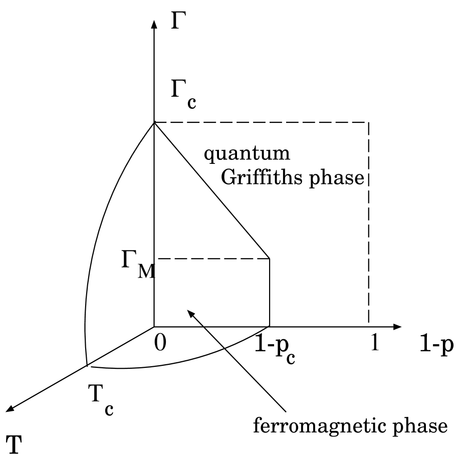
Fig.  5: Schematic phase diagram of the site diluted system.

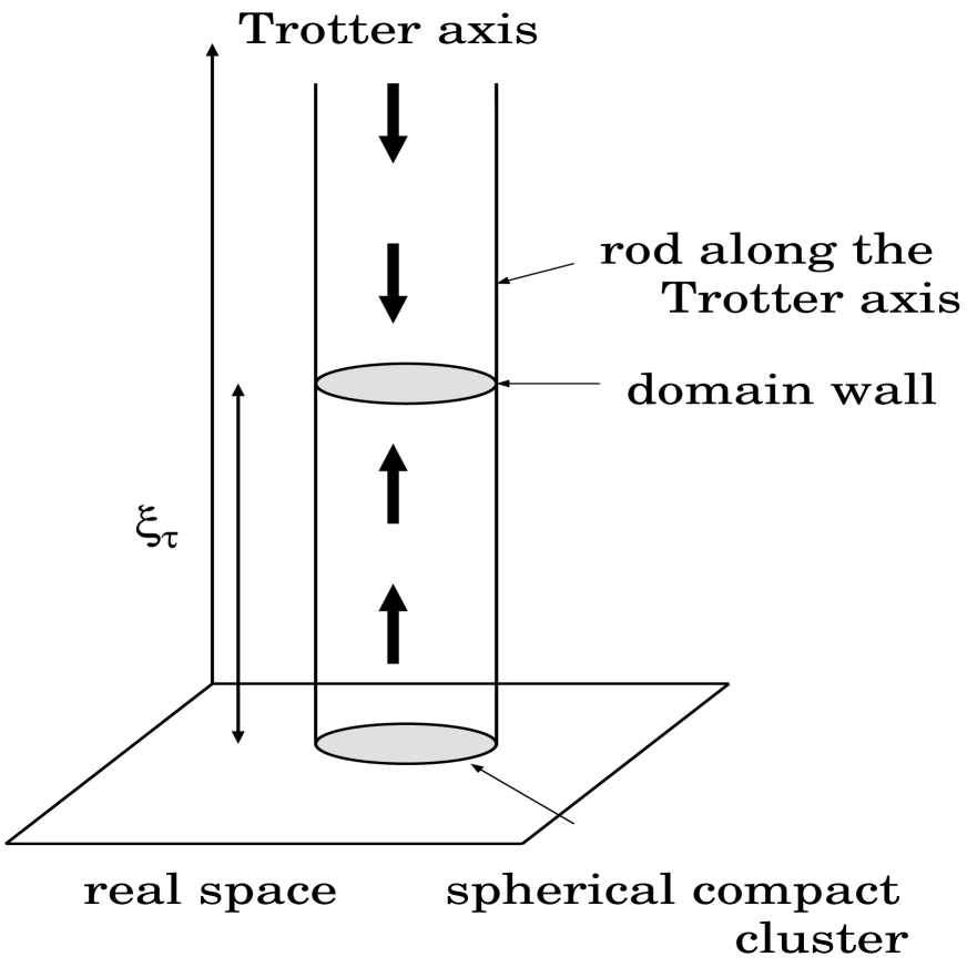
Fig.  6: Schematic picture of a local cluster which forms a rod along the the Trotter axis.

Fig.  7: Log-Log plot of the integrated distribution of the single site susceptibility $\chi_{local}$ at $\Gamma=0.7$, $p=0.30$. In this case, we evaluate the distribution using $100$ different $20\times 20$ configurations. The dotted line is a fit to the straight line region of the data and has the slope $-0.416$.

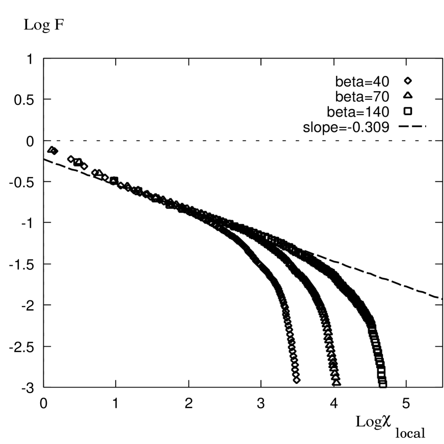
Fig.  8: Similar to Fig. 6 but for $\Gamma=1.0$, $p=0.40$. In this case, we evaluate the distribution using $100$ different $20\times 20$ configurations. The slope of the straight line is $-0.309$.

Fig.  9: Similar to Fig. 6 but for $\Gamma=1.5$, $p=0.50$. In this case, we evaluate the distribution using $100$ different $20\times 20$ configurations. The slope of the straight line is $-0.512$.

Fig.  10: Similar to Fig. 6 but for $\Gamma=2.0$, $p=0.66$. In this case, we evaluate the distribution using $100$ different $20\times 20$ configurations. The slope of the straight line is -0.391.

Fig.  11: Plot of $d/z$ obtained by fitting the integrated distribution $F\left(\chi_{local}\right)$ for various $\Gamma$. For $\Gamma=0.7$ and $1.0$, $d/z$ vanish at $p\simeq p_{c}$, but, for $\Gamma=1.5$ and $2.0$, these vanish at $p>p_{c}$. When $z>d$, the average susceptibility will diverge.

Fig.  12: Extraction of the exponent from the data for $d/z$ for $\Gamma=0.7$ and $1.0$, in which, $\Delta p$ implies $|p-p_{c}|$ ($p_{c}$ is $0.59$, the known percolation threshold). The value of $D\nu_{p}$ obtained from the percolation theory is known as $D\nu_{p}\simeq 2.57$, and the criticality of $d/z$ seems to be indeed compatible with the relation (21).

References

- [1] Bikas K. Chakrabarti, Amit Dutta and Parongama Sen, Quantum Ising Phase and Transverse Ising Models (Springer, 1996).
- [2] See H. Rieger and A. P Young, in Complex Behavior of Glassy Systems, ed. M. Rubi and C. Perez-Vicente, Lecture Notes in Physics 492, p. 256, Springer-Verlag, Heidelberg, 1997, for a review.
- [3] R.B. Griffiths, Phys. Rev. Lett. 23, 17 (1969).
- [4] B. McCoy, Phys. Rev. Lett. 23, 383 (1969).
- [5] C. Domb and S. Green, Phase Transitions and Critical Phenomena, (Academic Press) Vol.1.
- [6] M. Randeria, J. P. Sethna and R. G. Palmer, Phys. Rev. Lett. 54 (1985) 1321.
- [7] A. J. Bray, Phys. Rev. Lett. 54, (1988) 720.
- [8] H. Takano and S. Miyashita, J. Phys. Soc. Jpn. 58, (1989) 3871.
- [9] D.S. Fisher, Phys. Rev. Lett. 69, 534 (1992); Phys. Rev. B 51, 6411 (1995).
- [10] M. J. Thill and D. A. Huse, Physica A 15, 321 (1995).
- [11] H. Rieger and A. P. Young, Phys. Rev. B. 54, 3328 (1996).
- [12] M. Guo, R. N. Bhatt, and D. A. Huse, Phys. Rev. B. 54, 3336 (1996).
- [13] H. Rieger and A. P. Young, Phys. Rev. B. 53, 8486 (1996).
- [14] H. Rieger and N. Kawashima, cond-mat/9802104 (1998).
-
[15]
B. B. Beard and U. J. Wiese, Phys. Rev. Lett. 77, 5130 (1996),
N. V. Prokof’ev, B. V. Svistunov, I. S. Tupistyn, JETP Letters 64, 911 (1996); cond-mat/9703200 (1997),
B. B. Beard, R. J. Birgeneau, M. Greven, and U. J. Wiese, Phys. Rev. Lett. 80, 1742 (1998),
M. Troyer and M. Imada, (unpublished). - [16] T. Senthil and S. Sachdev, Phys. Rev. Lett.77, 5292 (1996).
-
[17]
H. Rieger and A. P. Young, Phys. Rev. Lett. 72, 4141 (1994),
M. Guo, R. N. Bhatt, and D. A. Huse, Phys. Rev. Lett. 72, 4137 (1994). - [18] B. Harris, J. Phys. C 7, 3082 (1974).
- [19] R. B. Stinchcombe, J. Phys. C 14, L263 (1981).
- [20] S. Bhattacharya and P. Ray, Phys. Lett 101A, 346 (1984).
- [21] M. Suzuki, Prog. Theor. Phys. 56, 1454 (1976); M. Suzuki in Quantum Monte Carlo Methods, Ed. M. Suzuki, Springer-Verlag, Heidelberg, p. 1 (1987).
- [22] R. J. Elliott and C. Wood, J. Phys. C 4, 2359 (1971).
- [23] P. Pfeuty and R. J. Elliott, J. Phys. C 4, 2370 (1971).
- [24] R. M. Ziff, Phys. Rev. Lett. 69, 2670 (1992).
- [25] D. Stauffer and A. Aharony, Introduction to percolation theory (Taylor and Francis, London, 1992).