Noisy time series generation by feed-forward networks

Abstract

We study the properties of a noisy time series generated by a continuous-valued feed-forward network in which the next input vector is determined from past output values. Numerical simulations of a perceptron-type network exhibit the expected broadening of the noise-free attractor, without changing the attractor dimension. We show that the broadening of the attractor due to the noise scales inversely with the size of the system ,$N$, as $1/\sqrt{N}$. We show both analytically and numerically that the diffusion constant for the phase along the attractor scales inversely with $N$. Hence, phase coherence holds up to a time that scales linearly with the size of the system. We find that the mean first passage time, $t$, to switch between attractors depends on $N$, and the reduced distance from bifurcation $\tau$ as $t=a{N\over\tau}\exp(b\tau N^{1/2})$, where $b$ is a constant which depends on the amplitude of the external noise. This result is obtained analytically for small $\tau$ and confirmed by numerical simulations.

]

I Introduction

The application of neural networks to the field of time series, covers several areas such as prediction [1], identification and control [2, 3]. The problem of time series prediction was well studied in the past [3] in the context of linear modeling, and later was extended to non-linear models. In this paper we analyze a typical class of architectures used in this field in the presence of additive noise, i.e. a feed-forward network governed by the following dynamic rule:

$$S_{1}^{t+1}=S_{out}^{t}+\mbox{noise}\quad;\qquad S_{j}^{t+1}=S_{j-1}^{t}\quad j=2,\ldots,N$$ (1)

where $S_{out}^{t}$ is the network’s output at time step $t$ and $S_{j}^{t}$ are the inputs at that time; $N$ is the size of the delayed input vector. The focus is set on the long-time (asymptotic) properties of the sequences generated by the system under the given dynamic rule. The clean model (without the additive noise) has been investigated [4, 5] and the main results are summarized below.

Since a realistic time series is noisy, it is imperative to understand the effect of noise on the output of the model. In this paper, we conduct an extensive quantitative study of the effect of noise on this particular class of model networks. We restrict the analysis to non-chaotic behaviour for two main reasons. First, chaotic behaviour does not allow long term prediction due to divergence of nearby trajectories, though such model networks are capable of generating chaotic sequences. Second, non-linear complex (however non-chaotic) time series are an important subclass which impose interesting questions. Hence understanding the relation between such complex behaviour and the architecture of the network is crucial form the point of view of time series prediction.

The basis for using time delayed vectors as inputs is the theory of state space reconstruction of a dynamic system using delay coordinates [6, 7]. An architecture incorporating time delays is the TDNN - time-delay neural network [8], which when operates in the iterative mode contains a recurrent loop (as in the model described above, without noise). This type of networks is appropriate for learning temporal sequences, e.g. speech signal and for short term prediction. The model we investigate can be viewed as a degenerate form of a TDNN in which the delay-lines are restricted to the input layer. Note that the dynamic rule (equation 1) corresponds to the closed-loop mode of operation used for generating subsequent predictions iteratively once the network has been trained on a given time series. Though some work has been done on characterization of a dynamic system from its time series using neural networks, not much analytical results that connect architecture and long-time prediction are available (see M. Mozer in [1]). Nevertheless, practical considerations for choosing the architecture were investigated extensively (see [1] and references therein).

Recently, it has been shown [5] that an hierarchy among the complexity of time series generated by different architectures exists. This information can be used as a guideline for an application in the following way. Given a time series one can conclude some quantitative measures regarding the complexity of the sequence, e.g. the attractor dimension and choose an architecture for the prediction task which is high enough in the hierarchy to ensure that it is capable of generating such a complex sequence.

Let us review briefly the main findings of the clean model. For conciseness we shall refer to the model generating the sequence as a SGen - Sequence Generator. The simplest SGen consists of a perceptron (Figure 1) whose output at time $t$, $S_{out}^{t}$, is determined by the input vector at time $t$, $~{}\vec{S}^{t}~{}$, $~{}(\vec{S}^{t}=(S_{1}^{t},\ldots,S_{N}^{t}))~{}$ as follows:

$$S_{out}^{t}=\tanh(\beta{\vec{J}}\cdot{\vec{S}}^{t})$$ (2)

for a fixed weight vector $~{}\vec{J}~{}$ and gain $\beta$. The input vector $~{}\vec{S}^{t}~{}$ is given by:

$$S_{i}^{t}=S_{out}^{t-i}~{},~{}~{}i=1\ldots N$$ (3)

i.e. the inputs are chosen to be the output values at the previous $N$ times. Thus, starting from an initial state $~{}S_{i}=S_{i}^{0},~{}i=1\ldots N$ the system generates the sequence $~{}S^{t}~{},~{}t=1,2,\ldots~{}~{}$ as follows:

$$S^{t}=\tanh(\beta\sum_{i=1}^{N}J_{i}S^{t-i})$$ (4)

FIG. 1.: SGen generating a time series.

In the case of a generic perceptron-SGen, the system is attracted into a quasi-periodic (QP) flow governed by one of the Fourier components of the power spectrum (PS) of the weight vector. Hence, the attractor dimension ($AD$) is one. Denoting the frequency and phase of the governing Fourier component by $K$ and $\phi$ respectively, the corresponding part in the weight vector is $~{}J_{i}=R\cos({2\pi\over N}Ki-\pi\phi)~{}~{}$, and the dynamic solution in the leading order of $N$ and $~{}1\ll K\ll N~{}$ is of the form:

$$S^{t}=\tanh\left[A\cos({2\pi\over N}(K-\phi)t)\right]$$ (5)

The amplitude $(A)$ of this solution depends on the gain $(\beta)$ and the phase $(\phi)$ in the following way:

$$N\beta=\frac{\pi\phi}{R\sin\pi\phi}\left[\sum_{\rho=1}^{\infty}{A^{2\rho-2}\over(\rho!)^{2}}(2^{2\rho}-1)B_{2\rho}\right]^{-1}$$ (6)

where $B_{\rho}$ are the Bernoulli numbers. Note that $A$ vanishes below a critical value ( which depends both on the amplitude of the weight vector $(R)$ and its phase $(\phi)$ ) $~{}\beta_{c}={2\over RN}{\pi\phi\over\sin(\pi\phi)}~{}$, indicating that the system undergoes a Hopf bifurcation at $~{}\beta_{c}~{}$.

In the more involved case the model consists of a MLN - Multi-Layer Network. The solution is a combination of perceptron-like SGen solutions. The exact details, however, depend on $\beta$ and the specification of the weight vectors (for more details see [5]). The $AD$ in the generic case is bounded by the number of hidden units connected to the input layer. Moreover, in [9] it was shown that the typical relaxation time for such a system from an arbitrary initial condition is proportional to the size of the delayed input vector. This result is of importance for time series prediction by setting a bound on the horizon of predictions.

The problem of noise in a dynamic system is of great importance for the behaviour of the system (e.g. stability), and hence its implications on the time series measured from that system. In the classical theory of time series analysis (linear and non-linear), one is interested in the prediction ability of a model when trained with noisy data. Since one intends to use a SGen to reproduce noisy data, it is important to understand how noise affects the output of a generic SGen. In particular, it is crucial that the SGen be robust under the addition of noise, which is non-trivial given the non-linear feedback dynamics of the SGen. The addition of noise enables us to check the stability of the previous results, obtained for isolated models.

As we shall see, the SGen is indeed extremely stable in the presence of noise. The noise causes the attractor to broaden. Even large noise of order the signal does not destroy the attractor. This gives rise to several quantitative issues. In section III we focus on a perceptron-SGen with one Fourier component in its weight vector. First, we analyze the scaling with $N$ of the manner in which the attractor is broadened due to the noise. This quantity manifests the cooperative aspect of the degrees of freedom in the system. We show that the broadening increases with $N$ as $1/\sqrt{N}$. Next, we discuss the issue of phase coherence (PC). Loss of PC is a generic phenomenon for periodic systems perturbed by noise. In this section, we analyze the extent to which adding noise to the SGen reduces its PC. The analysis is done for two types of dynamic rules, namely sequential updating (described above) and parallel updating (see section II). We show that the phase behaves as a biased random walk process, as typically observed in noisy oscillators, however the diffusion coefficient $D$ exhibits a power-law dependency on $N$. For the sequential (parallel) rule, $D\sim 1/N^{2}~{}(1/N)$. The importance of this result is that for large systems, PC is lost only over times that scale with the size of the system. This lost of PC also leads to a broadening of the dominant component in the power spectrum. We observe that this broadening decreases with $N$, consistent with the decrease of $D$ with $N$ discussed above.

Next, we measure the $AD$ of the broadened attractor. As mentioned before, we focus on the classification of various SGen’s by the long term sequence they produce, therefore we are interested in the estimation of this quantity. In section IV we apply standard methods to estimate the $AD$ of time series generated by the SGen. With no noise added, we of course recover the analytical results, e.g. $AD=1$ for the perceptron-SGen. The more important question is how the noise added to the system influences the measured $AD$. Our treatment parallels that found in the literature of dynamic systems where the $AD$ was estimated from a measured (noisy) time series taken from chaotic systems or strange attractors [10, 11]. We measure the $AD$ of a perceptron-SGen, as well as of a Committee Machine whose parameters were chosen in such a way that two Fourier components have a non-zero coefficient and whose $AD$, therefore, should equal $2$. We found that for length scales greater than the typical size of the noise and well below the attractor’s radius, the $AD$ of the SGen does not differ from the expected analytical results.

Finally, in section V we analyze the effect of noise on a SGen with multiple attractors. While in the non-noisy case, the perceptron-SGen exhibits a single stable attractor, here we expect transitions between attractors due to the noise. We focus on the average time needed to escape from a basin of attraction, and particularly its dependence on the sizes of both the system and the attractor. This quantity, also known as the mean first passage time, has been investigated extensively in the context of chemical reactions, dynamical systems etc. [12, 13, 14]. Obviously, we are interested in the case of a discrete system. This issue has been less treated (see [12] and [15]). We consider the case of a system governed by two Fourier components that results in two attractors. The problem of escape time is related to the evolution of the amplitude in coupled map equations. The phase portrait of such a map suggests that the motion in this phase space can be approximated by a one dimensional flow of the form:

$$x_{n+1}=f(x_{n})+\xi_{n}$$ (7)

where $f(x)$ is a non-linear map and $\xi$ is the noise term. Following the treatment of Talkner et al. [13], we relate our system to the problem of a discrete dynamics with small non-linearity in the presence of a weak noise. The analytical result is in a good agreement with extensive simulations of the perceptron-SGen for both the polynomial prefactor and the leading exponential part.

The results presented herein will primarily focus on the perceptron-SGen. Nevertheless we expect that the general properties and trends remain true in the more general case.

Summary and a discussion are presented in section VI.

II Preliminaries

Let us introduce a few concepts which are of general use in the following. The basic model is the SGen in its simplest form - a perceptron whose output is connected to the first input, as described in the previous section. This is the sequential updating rule, given by eqs. 2 - 4.

The sequential scheme can be thought of as a fully connected network with $N+1$ units. The units are updated one at a time, i.e. at each time step, another unit plays the role of an output unit. The weight matrix connecting the units is asymmetric with a certain spatial structure where the interactions are only a function of the difference between the location of each pair of units ($ij$):

$$J_{ij}=W_{i-j~{}\mbox{mod}~{}N+1}$$ (8)

where $W_{0}=0$, and $W_{l}~{}(l\neq 0)~{}$ is the same weight vector of the sequential rule. The main diagonal elements are zero, and the rest are the same values as the first row but cyclically permuted, e.g. for $N=3$:

$${\bf J}=\left[\begin{array}[]{cccc}0&W_{1}&W_{2}&W_{3}\\ W_{3}&0&W_{1}&W_{2}\\ W_{2}&W_{3}&0&W_{1}\\ W_{1}&W_{2}&W_{3}&0\end{array}\right]$$ (9)

This type of weight matrix is said to have a Toeplitz structure. To implement the parallel scheme, all the units are updated simultaneously with the sequential rule via the matrix described in equation 8:

$$S_{i}^{t+1}=\tanh(\beta\sum_{j=1}^{N+1}J_{ij}S_{j}^{t})$$ (10)

In the sequential scheme, noise is presented to the system in the following way:

$$S_{1}^{t+1}=S_{out}^{t}+\eta^{t}.$$ (11)

where $\eta$ is distributed according to:

$$E[\eta^{t}] = 0.$$ (12)

$$E[\eta^{t}\eta^{t^{\prime}}] = \sigma^{2}\delta_{tt^{\prime}}.$$ (13)

In this way, noise is added only to the first unit in each iteration of the dynamic rule. In the parallel updating scheme, the noise is represented by a vector with $N+1$ independent components ${\vec{\eta}}^{t}$, which is added to all units simultaneously in each iteration:

$$S_{i}^{t+1}=\tanh(\beta\sum_{j=1}^{N+1}J_{ij}S_{j}^{t})+\eta^{t}_{i}$$ (14)

As we previously noted, the sequential SGen produces a time series which can be denoted by $S^{t}$, $~{}~{}t=1,2,\ldots~{}$. The sequence $S^{t}$ is the basis of the numerical analysis. In order to use the rich theory of reconstructing state space [6, 7], one has to embed the time series in a phase space. The process of embedding a time series onto a d-dimensional space, generates a set of vectors (or a trajectory) in that space. The embedded vectors are:

$${\bf\vec{X}_{t}}=(S^{t},S^{t-1},\ldots,S^{t-d+1})$$ (15)

III Properties of a single attractor

In this section, we analyze the properties of a perceptron-like SGen with a weight vector that contains a single Fourier component with an arbitrary phase $(\phi)$ of the form $~{}~{}J_{j}=R\cos\left({2\pi\over N}Kj-\pi\phi\right)~{}$. When no noise is added to the dynamic equation (equation 4), the generic stable solution was found to be a quasi-periodic orbit [5], e.g. Figure 2.

FIG. 2.: Quasi-periodic orbit generated by a perceptron $N=50,~{}K=17,~{}\beta=1/17,~{}\phi=.123$.

When noise is added (equation 11), the orbit is broadened. Nevertheless, the system does not become ergodic and the trajectory is confined in phase space. A characteristic quantity is the noise induced width of the broadened attractor. In the following we present both quantitative explanations and measurements of the dependence of this quantity on the size of the system $~{}N$. Next, we discuss the important issue of phase coherence. A periodic system in the presence of noise typically exhibits a loss of phase coherence. This is a result of the fundamental invariance of the system w.r.t. time translation, so there is no restoring force to a perturbation which induces a phase shift. As we shall see, this results in a broadening of the PS of the time series generated by the system.

A Attractor broadening

Let us define the width of the attractor $<W>$ to be the average local broadening of the embedded time series, see Figure 3.

FIG. 3.: Same parameters as previous figure but with a uniform noise of amplitude $\pm 0.1$ added.

In this case, we embed the data in a two dimensional space and measure the extent perpendicular to the local tangent. Having done this for a system of sizes $N=20,50,100,200$, we plot $<W>$ (denoted by $<$ width $>$ in the figure) vs. $N$ in Figure 4. There exists a clear power-law scaling between the two quantities of the form $W\propto A/\sqrt{N}$ where $A$ is a constant.

FIG. 4.: The average width of the embedded time series. The power-law fit (dashed line) is $0.15/N^{\alpha}$ , $\alpha=0.5\pm 0.007$

To understand this scaling law, consider a random vector (RV) in a $N$-dimensional space. The relevant quantity is the projection of such a RV on a fixed vector - the weight vector $\vec{J}$. Denote the output field $h$ as a sum of projections resulting from the stable solution vector $\vec{S}$ and the noise vector $\vec{\eta}$ :

$$h=\vec{J}\cdot(\vec{S}+\vec{\eta})\equiv x_{s}+x_{n}.$$ (16)

The components of $\vec{\eta}$ are the last $N$ noise terms given by equation 11. The output value is then $~{}S_{out}=\tanh\left[\beta h\right]~{}$. In writing equation 16 we neglect contributions from noise terms after iterations of the map, as these corrections are proportional to $\beta$ and so are ${\cal O}(1/N)$. This can be justified as long as the parameter $\beta$ can be written as

$$\beta=(1+b)\beta_{c}$$ (17)

and $b$ does not scale with $N$. The term $x_{s}$ is of $~{}{\cal O}(N)~{}$ as this is the exact solution without noise. The term $x_{n}~{}$ is the focus of our interest. Since the $\eta_{i}$ components are RV’s , we can calculate the first two moments of $x_{n}$:

$$E(x_{n}) = \sum_{i=1}^{N}J_{i}E(\eta_{i})=0$$ (18)

$$E(x_{n}^{2}) = \sum_{i,j}J_{i}J_{j}E(\eta_{i}\eta_{j})=\sum_{i,j}J_{i}J_{j}\sigma^{2}\delta_{ij}=\sigma^{2}\frac{N}{2}$$ (19)

Thus the variance of the noise term is of ${\cal O}(N)$. The geometrical interpretation is that a RV has a projection which is of ${\cal O}(\sqrt{N})$ on a given direction. Since the parameter $\beta$ scales as $~{}1/N~{}$ (as long as $b$ in equation 17 does not scale with $N$), we can conclude that the contribution of the noise term scales as $~{}1/\sqrt{N}$, in agreement with the numerical results presented above. Note that this results hold even for large noise values and are linear with $(\sigma)$.

B Phase coherency

On general grounds, we expect the phase to undergo a biased random walk, where the bias represents the frequency of the unperturbed system. We can measure this directly by comparing the phase of the noisy system to that of a noise-free “reference” system. Starting from identical initial conditions, the accumulated phase in each series is measured. Denoting the accumulated phase in the clean/noisy series (subscript $c,n$) at time $t$ by:

$$\Phi_{c}(t) = \sum_{i=0}^{t}\left(\phi_{c}(i+1)-\phi_{c}(i)\right)~{}~{}~{}~{}~{}~{}\phi_{c}(0)=\phi_{n}(0)$$ (20)

$$\Phi_{n}(t) = \sum_{i=0}^{t}\left(\phi_{n}(i+1)-\phi_{n}(i)\right)$$ (21)

FIG. 5.: Relative phases of the embedded vectors. The left part of the figure describes a “clean” point surrounded by typical noisy points.

where the phases $~{}\phi_{c}(i)~{},\phi_{n}(i)~{}$ are the relative phases of the i’th clean/noisy embedded vectors w.r.t. an arbitrary, but fixed, coordinate system (see Figure 5, ignore the left part of the figure). The quantity of interest is the expectation value of the squared phase difference defined by:

$$\left<\Delta\Phi^{2}(t)\right>=E\left[(\Phi_{c}(t)-\Phi_{n}(t))^{2}\right]$$ (22)

where $~{}<\bullet>~{}$ stands for the average over all samples taken after the same time $t$.

An example of the quantity defined in equation 22 is given in Figure 6. Clearly, this behaviour indicates that the process is diffusive.

FIG. 6.: Example of the behaviour of the variance of the phase difference over time. The slope (dashed line) is the linear regression.

The slope of this figure represents the diffusion coefficient. The diffusion coefficient was extracted from data of the type represented in Figure 6 for both parallel and sequential updating rules. Each data point is an average over $400$ samples (as in the figure). In each case, the simulations were taken at different system sizes. The exact parameters of each SGen are not important, however they were chosen such that the solution is QP and well above the critical value $\beta_{c}$ where a bifurcation occurs. Each point in Figures 7,8, is the slope of the linear regression and the statistical error is less than the size of the point. The results from the figures reveal a scaling law of the diffusion coefficient $D$:

$$D\sim 1/N^{a}$$ (23)

where $a=1(2)$ for the parallel (sequential) rule.

FIG. 7.: Diffusion coefficient for the parallel rule. The linear regression (dashed line) is $~{}D=0.029/N^{a}\,\mbox{\,with\,}a=1\pm 0.03$.

FIG. 8.: Diffusion coefficient for the sequential rule. The linear regression (dashed line) is $~{}D=0.154/N^{a}\,\mbox{\,with\,}a=2\pm 0.036$.

To understand these results, let us now extend the arguments that led to the “width” of the noise in the previous section. We start with the parallel dynamics and develop a relation between $~{}\left<\Delta\Phi^{2}(t)\right>~{}$ and time. It was shown that the contribution of the noise is of the order $~{}1/\sqrt{N}~{}$. Examine Figure 5 (its left part) in the context of Figures 2,3. Each point along the clean orbit, is surrounded by a cloud whose typical radius is of ${\cal O}(1/\sqrt{N})$. So basically, the distance between one iteration of the same point in the clean and the noisy series, is of ${\cal O}(1/\sqrt{N})$. Since the noise is assumed to be small, the phase can be approximated by the distance projected on the QP orbit. Hence, the variance of that phase scales as $1/N$. This explains the result for the scaling law in the parallel case. The sequential dynamics has the same characteristics, however the time steps should be rescaled w.r.t. the parallel dynamics by a factor of $1/N$. That is the reason for the $1/N^{2}$ scaling.

One can conclude that phase diffusion indeed occurs (as expected), however its associated time scale increases with the size of the system in a power-law fashion (equation 23). Therefore the system remains coherent over increasingly long times as $N$ increases.

The loss of PC is also manifested in the Fourier domain in the broadening of the dominant Fourier component. In the unperturbed system, the power spectrum of the stable solution/state is characterized by a sharp peak (delta function). The noisy system produces a sequence whose power spectrum is broadened around the unperturbed Fourier component. The larger the phase diffusion constant $D$, the more broadened the dominant component. We indeed observe that the broadening decreases with $N$. Figure 9 depicts the power spectrum of two sequences (of the same length) generated by two perceptron-SGen of sizes $N=32,128$. The wave number of the single Fourier component is $K=7$ and the weight vector is produced according to: $~{}J_{i}=\cos({2\pi\over N}Ki)~{},~{}~{}i=1\ldots N~{}$. The power axis is drawn in a log scale to emphasize the broadening effect.

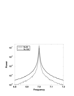
FIG. 9.: Broadening of the dominant component in the power spectrum. The weight vector consists of one Fourier component with $K=7$. The systems sizes are $N=32,128$.

IV Attractor dimension

We have seen that in the case of the perceptron-SGen, the noise gave rise to a broadening of the attractor. The attractor, nonetheless remained essentially 1-dimensional, as a perusal of figures 2,3 immediately verifies. This is consistent with the general behaviour of simple attractors in the presence of noise. For the case of the MLN, we expect the general picture to persist. It is however non-trivial to verify this since the attractor is higher dimensional. We employ for this purpose the tools that have been developed for analysing dynamical systems from their time series. Of course, the question of attractor dimension is crucial for exploiting these networks for prediction and modeling.

Many methods were proposed for estimating the $AD$. We just mention the simplest method, which is the ”Box-Counting” [16]. In fact, most methods are based on statistical estimators for the dimensionality of the attractor. We used the Correlation-Integral method, that was introduced by Grassberger and Procaccia [17] (see also [18, 19]). In this method the $AD$, denoted by $D$, is estimated by calculating the correlation sum $C(r)$ from the data as follows:

$$D=\lim_{\stackrel{{\scriptstyle N_{p}\rightarrow\infty}}{{r\rightarrow 0}}}\frac{\ln C(r)}{\ln r}$$ (24)

where :

$$C(r)=\frac{1}{N_{p}^{2}}\sum_{i,j=1}^{N_{p}}\Theta\left(r-\left|\vec{X_{i}}-\vec{X_{j}}\right|\right)$$ (25)

$\vec{X_{i}}$ are the embedded time series vectors (equation 15), $N_{p}$ is the number of data points and $\Theta$ is the Heaviside step function.

In practice, the $AD$ is estimated in the so-called scaling region of the correlation integral, i.e.  one has to identify a sufficiently large range of lengths scales over which the slope is constant. In many cases, the picture is not very clear especially when the number of points is not large enough, or when certain parameters in the algorithm for estimating $C(r)$ are not optimized (e.g. delay time) [20, 21]. We also note that since the data has a high degree of correlation, one has to introduce a cut-off to exclude points that were generated closer (in time) than this value [21]. This points have strong correlation that affect the correlation dimension which measures the correlation between points from different passes of the trajectory. We used the first zero of the autocorrelation function as a cut-off.

When the measurements are corrupted with noise one can distinguish between two regimes of length scales; one dominated by the attractor and the other by the noise. This problem was originally investigated by Mizrachi et al. [10], and Zardecki [11]. In the broad sense, one can identify four regions [22]. Due to the finite number of points in the data sample, for very small $r$, the number of points in the sphere of radius $r$ approaches zero, and hence also the slope. At larger $r$, there is a transition to a region where the noise dominates. If the number of points is large enough, the slope saturates the embedding dimension. At yet larger $r$, one enters the scaling region with a constant slope estimating the $AD$ (given that the region is large enough). Finally, the slope returns to zero as $r$ reaches the attractor’s radius. For clarity only the second and third regions are shown.

Let us now describe our measurements. The time series were generated for four cases: a perceptron without noise (Figure 10); perceptron with noise added as described in equation 11 (Figure 12); and a Committee Machine (CM) with three hidden units with and without noise (Figures 11,13). By a CM we mean a two-layered network whose second layer weights equal one. Each perceptron in the hidden layer (as well as the perceptron-SGen) has only one Fourier component in its weight vector and an arbitrary phase :

$$J_{j}^{h}=R_{h}\cos\left({2\pi\over N}K_{h}j-\pi\phi_{h}\right)$$ (26)

where $R$ is an amplitude, $N$ is the input size, $K$ is the wave number, $\phi$ is a constant phase shift and $h$ labels the hidden unit. ( The case of more than one Fourier component is treated in a different context in section V ). The gain parameter $\beta$ in the CM was chosen so that the stable attractor of this SGen contains only two components in the power spectrum. This choice produces a $2D$ attractor. (The values of all the parameters are given in the figure captions).

The figures present the calculated $~{}~{}\ln C_{2}(r)~{}$. The $AD$ is estimated by the local slope,   $d[\ln\,C_{2}(r)]/d[\ln\,r]~{}~{}$ and presented in the insert. It is important to note that all data points are rescaled to the region $[0,1]$, prior to the evaluation of the correlation integral. Figure 10 presents results for the simplest perceptron-SGen with only one Fourier component in its weight vector. The arbitrary chosen phase shift $\phi$ results in a QP orbit [5] which is $1D$ ($AD=1$). We embedded the time series in $m=2,3~{}\mbox{and}~{}4$ dimensional spaces. Clearly the measurements support the analytical results and the $AD$ measured is about $AD=1.01$. In Figure 11, we present the results for the more complicated attractor generated by the CM. The expected $AD$ is $2~{}$ (as described above). The results are slightly above 2, that is $2.0<AD<2.03$. Notice that the embedding in a 2D-space gives a wrong result, as expected, since the structure of the attractor is unfolded only in a 3D space, at least.

FIG. 10.: Perceptron without noise. $N=400$, $\beta=1/180$, $\phi=0.2235$ $R=1.0$. The solid guide line in the insert is at $1.01$. $(\circ~{}m=2,~{}\Box~{}m=3,~{}\Diamond~{}m=4)$.

FIG. 11.: CM that exhibits a 2D attractor, without noise. $N=500$, $\beta=1/185$, $\phi_{i}=0.2235,0.3524,0.4244.~{}R_{i}=1.0~{}$, $i=1,2,3$. The solid guide line in the insert is at $2.02$. $(\circ~{}m=2,~{}\Box~{}m=3,~{}\Diamond~{}m=4)$.

Now we analyze the same perceptron-SGen and CM but with noise added (see Figures 12, 13). We embedded the time series as in the non-noisy case in $m=2,3$ and $4$ dimensional spaces. We used a uniformly distributed noise with an amplitude of $\pm 10^{-2}$ while the attractor’s amplitude is bounded by $\pm 0.7(\pm 1.2)$ for the perceptron (CM), prior to rescaling. Our results are similar to other noisy dynamic systems [10] in the sense that for length greater then the characteristic noise scale, the measured $AD$ saturates the true dimensionality, i.e. in this case $AD=1(2)$ (as in the non-noisy case). However below that scale, the noise dominates and since in general it fills the space in all dimensions, the slope increases with the embedded dimension. In our case, the slope measured for the noise is correct only in $m=2,3$, while in higher dimensions it is lower than the embedded dimension. The reason for this inaccuracy is that we have not used enough points so the space was not filled densely by the noise. The results are $AD\sim 1.01(2.07)$ which are slightly higher than the non-noisy case for the CM.

FIG. 12.: Perceptron with noise added. $N=100$, $\beta=1/40$, $\phi=0.2235$, $R=1.0$. The solid guide line in the insert is at $1.01$. $(\circ~{}m=2,~{}\Box~{}m=3,~{}\Diamond~{}m=4)$.

FIG. 13.: CM that exhibits a 2D attractor, with noise added. $N=500$, $\beta=1/185$, $\phi_{i}=0.2235,0.3524,0.4244.~{}R_{i}=1.0~{}$ , $i=1,2,3$. The solid guide line in the insert is at $2.07$. $(\circ~{}m=2,~{}\Box~{}m=3,~{}\Diamond~{}m=4)$.

In all the figures, one can easily identify the scaling region which is quite broad, more than an order of magnitude of length. The conclusion from the results is that the SGen maintains its $AD$ in the presence of noise. The effect of noise is bounded to small length scales, as expected.

V Escape from a meta-stable attractor

So far, we have discussed several properties of the dynamics in the neighborhood of a single attractor. This section is devoted to the analysis of the dynamics when there are multiple attractors. In particular, we focus on the average time to escape from the domain of one of the attractors. The picture one should have in mind is of several states having local stability with transitions between them induced by noise.

In the first section we derive an analytical result for the mean first passage time (MFPT) in the limit of weak noise and a weakly non-linear map. The reasons for taking these limits will be explained later. The second section describes a series of simulations which support the analytical results.

A The mean first passage time in periodic attractors

In the following we analyze the case where each of the meta-stable states is characterized by an N-states periodic attractor. This property is achieved by setting the phase shift $\phi$ (e.g. equation 26) to zero [5]. In order to keep the discussion as simple as possible, let us restrict ourselves to the case of a perceptron-SGen with two Fourier components in the power spectrum of the weight vector. Hence, the weight vector is given by:

$$J_{j}=\sum_{m=1}^{2}R_{m}\cos({2\pi\over N}K_{m}j)$$ (27)

1 A simplified model

The key point is our ability to identify a low dimensional discrete dynamics that describes the evolution of the solution, and relate it to our problem of the SGen. In [5] it has been shown that the general solution for a perceptron-SGen with a weight vector defined by equation 27, is of the form:

$$s^{t}=\tanh[\sum_{m=1}^{2}A_{m}\cos(~{}{2\pi\over N}k_{m}t~{})]$$ (28)

This solution leads to self-consistent coupled equations for the amplitudes of the dynamic solution:

$$A_{m}^{n+1}=\beta NR_{m}\sum_{\rho=1}^{\infty}C(\rho)\sum_{t=0}^{\rho-1}{(A_{m}^{n})^{2t+1}(A_{m^{\prime}}^{n})^{2\rho-2t-2}\over(t+1)!t!(\rho-t-1)!^{2}}$$ (29)

where $n$ labels the discrete time, $C(\rho)\equiv(2^{2\rho}-1)B_{2\rho}/\rho$ ($B_{\rho}$ are the Bernoulli numbers), and $m^{\prime}=2$ for $m=1$ and vice-versa.

In the absence of noise, the coupled equations evolve into one of the two fixed points (f.p.’s) in which only one of the Fourier components has a non-vanishing coefficient. The addition of noise, as described in equation 11, generates a perturbation in each of the coupled equations. The perturbation can “kick” the system out of the vicinity of one stable f.p. so that it escape to the other f.p. We are interested in the mean time for such an event to occur.

We assume $R_{1}=R_{2}=1$, i.e. the symmetric case. In order to continue, we truncate and transform the coupled equations (equation 29). For small amplitudes, one need keep terms only up to third order. The result becomes:

$$A_{m}^{n+1}=\beta\frac{N}{2}\left[A_{m}^{n}-\frac{1}{4}(A_{m}^{n})^{3}-\frac{1}{2}A_{m}^{n}(A_{m^{\prime}}^{n})^{2}\right]$$ (30)

where, as before, $m^{\prime}=2$ for $m=1$ and vice-versa. One can treat these equations as a recursive solution for the amplitudes of the dynamic solution. In this sense, equations 30 become discrete dynamic equations. For notational convenience we shall relabel the variables with $A_{1}\rightarrow x$ and $A_{2}\rightarrow y$. In addition, we introduce the reduced variable $\tau$ as follows:

$$\tau=\frac{\beta-\beta_{c}}{\beta_{c}}~{}~{}~{}\Longrightarrow~{}~{}~{}\beta\frac{N}{2}=1+\tau$$ (31)

where $\beta_{c}=2/N$. This redefinition allows us to rewrite equation 30 as an $N$-independent map:

$$x_{n+1}=(1+\tau)\left[x_{n}-\frac{1}{4}x_{n}^{3}-\frac{1}{2}x_{n}y_{n}^{2}\right]$$ (32)

The second equation is obtained by replacing $x$ by $y$ and vice-versa, $x\Leftrightarrow y$ .

Analysis of these equations under the assumption that $\tau\ll 1$, gives four symmetric f.p.’s, namely: $y^{\star}=0~{},~{}x^{\star}=\pm 2\sqrt{\tau}$ and vice-versa. These f.p.’s are stable and we consider only the positive ones. In addition, we have a trivial unstable f.p. and four saddle points at $~{}x_{sp}^{\pm},y_{sp}^{\pm}=\pm{2\sqrt{3}\over 3}\sqrt{\tau}~{}$. A typical phase portrait of this map is depicted in Figure 14 (actually, only the positive quadrant is shown). The stable f.p.’s are at $~{}x^{\star}=0.2~{},~{}y^{\star}=0~{}$ and $~{}y^{\star}=0~{},~{}x^{\star}=0.2~{}$ ( the other two symmetric f.p.’s are not shown ). The saddle point shown is at $~{}x_{sp}^{+},y_{sp}^{+}={0.2\sqrt{3}\over 3}~{}$, whereas the other three are not shown. Let us denote this point by $~{}SP^{+}~{}$, and with $~{}SP^{-}~{}$ denoting the other saddle point, i.e. $~{}(x_{sp}^{+},y_{sp}^{-})~{}$.

FIG. 14.: Phase portrait of the $2D$ map with $\tau=0.01$. SP denotes a saddle point.

The boundary between the two domains of attraction is clearly the line $x=y$. The additive noise, as mentioned above, perturbs these equations and as a result the system may escape from the domain of attraction defined by $x>y$. The random time it takes for the system to reach the state $x=y$ is the first passage time stochastic variable. Note that the additive noise described in equation 11 is not the same one used in our model here, since the first noise is applied directly to the SGen, while the second is the effect of such noise on the amplitude of the solution. The connection between the following model and the SGen is given in the next subsection.

The model for the perturbed system, is described by the following $2D$ noisy map:

$$x_{n+1}=(1+\tau)\left[x_{n}-\frac{1}{4}x_{n}^{3}-\frac{1}{2}x_{n}y_{n}^{2}\right]+\xi_{n}.$$ (33)

where $\xi_{n}$ is a Gaussian additive noise distributed according to:

$$\rho_{\epsilon}(\xi)=\frac{1}{(2\pi\epsilon)^{1/2}}\exp-\frac{\xi^{2}}{2\epsilon}$$ (34)

The map for $y$ is obtained in the same manner as in equation 32. Note that due to the mutual independence of the $\xi_{n}$, the process defined in equation 33 is a Markov process.

The region of interest is of ${\cal O}(\sqrt{\tau})$. Following an appropriate rescaling of equation 33, we get:

$$\tilde{x}_{n+1}=f(\tilde{x}_{n},\tilde{y}_{n})+\tilde{\xi}_{n}=\tilde{x}_{n}-\tau\left[-\tilde{x}_{n}+\frac{1}{4}\tilde{x}_{n}^{3}+\frac{1}{2}\tilde{x}_{n}\tilde{y}_{n}^{2}\right]+\tilde{\xi}_{n}~{}.$$ (35)

where $\tilde{x}_{n},\tilde{y}_{n},\tilde{\xi}_{n}$ are the rescaled variables. We further rewrite the map in the following way:

$$f(x_{n},y_{n})=x_{n}-\tau{\cal U^{\prime}}(x_{n},y_{n}).$$ (36)

The derivative is taken with respect to $x$ or $y$, depends on the variable for which the map is written for.

Say the initial condition is $y=0~{},~{}x=x^{\star}$, i.e. one of the f.p.’s. Since the line connecting this f.p. and the saddle point is a valley, we may assume that the most probable escape route is along this line (or its mirror through the x-axis, i.e. the line connecting the f.p. with the saddle point $(x_{sp}^{+},y_{sp}^{-})~{}$ ). This argument can be understood by rotating each noise term tangent and perpendicular to the path. The perpendicular term decays fast due to the restoring force, hence we can conjecture that the dynamics is mainly $1D$. Therefore, with the assumption of weak noise and $\tau\ll 1$ we can reduce the map into one dimension, on that path (for details, see [23]). Hence, a $1D$ noisy map is obtained:

$$s_{n+1}=s_{n}-\tau{\cal U^{\prime}}(s_{n})+\hat{\xi}_{n}~{}.$$ (37)

where $s$ defines the path. The noise term now is the tangential projection of the $2D$ noise on the path. The path $s$ can be found by writing an equation for $x(y)$ on the path, however the relation is implicit and cannot be used directly.

This type of a $1D$ equation has been investigated for the case of small non-linearity [13, 15, 24], namely, the class of map functions with the property that $f(x)$ deviates only weakly from the identity map:

$$f(x)=x-\tau\frac{dU(x)}{dx}~{},~{}~{}~{}~{}\tau\ll 1$$ (38)

The analogy with our $1D$ map (e.q. 37) is obvious. In the next section, we adapt the derivation of [24] to our map.

2 MFPT analysis

In the following, we sketch the calculation of the MFPT for the process defined in equation 37. The complete derivation and simulations will be given in [23].

Assume that the process described in equation 37 is defined in $(-\infty,\infty)$ and define the random variable $\tilde{t}(s)$, the first passage time from the interval $I=\left[SP^{-},SP^{+}\right]$ , by:

$$\tilde{t}=\min\{n:|s_{n}|\geq s_{sp}^{+}\}~{}.$$ (39)

i.e. the first time the process hit one of the boundaries, where $SP^{\pm}$ are the saddle points defined above, and $s_{sp}^{+}$ is the value of $s$ at the saddle point. The MFPT, $t(s)$, starting from a point in $I$ is given by:

$$t(s)=<\tilde{t}(s)>=E[~{}\tilde{t}~{}|~{}S_{0}=s~{}].$$ (40)

It was shown that the MFPT can be written as (e.g. [24]):

$$t(s)-1=\int_{I}P(z|s)t(z)dz$$ (41)

where $~{}P(z|s)~{}$ denote the transition probability to go from $s_{n}=s$ to $s_{n+1}=z$ in a single step. Under the assumption of weak noise $\epsilon\ll 1$, the function $t(s)$ is nearly constant inside the domain of attraction. Fluctuations occur mainly near the boundary. The reason is that only close to the boundary may one have a finite probability to jump over the boundary in small number of steps. Therefore, it was suggested [15, 24] that this function be written as a product of a constant value, and a boundary layer function:

$$t(s)=T\tilde{h}(s)~{}~{}~{}~{},~{}~{}\tilde{h}(s^{\star})=1$$ (42)

where $s^{\star}$ is the f.p. The boundary layer extends a distance of order ${\epsilon}^{1/2}$ around $s=s_{sp}^{+}$, and we can write the scaled boundary layer function $h(s)$, $h(s)=\tilde{h}((2\epsilon)^{1/2}s)$. Inserting this assumption in equation 41 gives an integral equation for $h(s)$. This equation was analytically solved by Talkner et al. [24] and by Knessl et al. [15]. The leading exponential part of the solution of this equation gives:

$$T\propto\exp\left[\frac{2\tau}{\epsilon}({\cal U}(SP^{+})-{\cal U}(s^{\star}))\right]$$ (43)

The potential difference has been calculated analytically (see [23]) and found to be $~{}{\cal U}(SP^{+})-{\cal U}(s^{\star})={1\over 3}$. The prefactor is obtained from integrals involving the boundary layer function. The final result for the MFPT reads:

$$T=\frac{a}{\tau}\exp\left(\frac{2}{3}\frac{\tau}{\epsilon}\right)$$ (44)

with $a$ constant.

Simulations of our $2D$ model (equation 35) are shown in Figure 15. The reduced variable $\tau$ is varied for different noise amplitudes $\epsilon$. The results are in excellent agreement with the prediction of the $1D$ theory (equation 44).

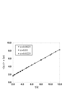
FIG. 15.: Scaling of the average logarithm of the escape time in the $2D$ model. The solid line is a linear regression and its slope is $0.658\pm 0.003$.

In the next sub-subsection we present the results from extensive simulations of the real system, i.e. the SGen.

B Numerical simulations

Measuring the MFPT directly from the time series generated by the noisy SGen is impossible, since there is no way to distinguish between the different attractors. The natural variable which does measure the projection of the current state on each attractor is the relative amplitude in the power spectrum of the input vector. Note that there exists an equivalence between the amplitudes of the solution to the coupled equations (equation 29) and the amplitude in the power spectrum of the corresponding Fourier components.

We study an SGen with a weight vector containing two Fourier components, as described at the beginning of the previous section, with no phase shift and both amplitudes equal to one, $R_{1}=R_{2}=1$. We applied the sequential updating scheme described in section II with a noise which is normally distributed ${\cal N}(\mu=0,\sigma=0.1)$. We set the initial conditions for each run to one of the Fourier components. In each experiment we measure the number of iterations before the amplitudes of the two components in the power spectrum of the input vector, become equal. As we expect an exponential behaviour of this quantity, we record the logarithm of the first passage time. We found that actually the average logarithm of the median first passage time has smaller variations than the average logarithm of the first passage time over all the data set. Each pair $(N,\tau)$ was tested $200-400$ times and the first passage time was recorded. The list of times was divided into $10$ groups and the average logarithm of the median from each group was taken. Finally, we end up with $10$ values from which we calculated the first and second moments.

Figure 16 depicts the ensemble of all experiments, in which we varied the size of the system in the range $200\leq N\leq 1500$ and the reduced variable $\tau$ in the range $~{}0.003<\tau<0.04~{}$. To demonstrate the scaling properties, we plot the average logarithm of the median escape time as a function of $\tau N^{\alpha}$. The worst error of the data points is about the size of the symbol, hence errors were omitted for clarity. Clearly, the average median time to escape follows the relation:

$$\left<t_{med}\right>=\frac{aN}{\tau}\exp(b\tau N^{\alpha})$$ (45)

where $~{}a,b,\alpha~{}$ are constants (given below).

FIG. 16.: Scaling of the average logarithm of the median escape time. The solid line is a linear regression and its slope is $11.2\pm 0.12$.

In order to appreciate this result, we need an appropriate variable transformation. Recall that in previous sections we saw that the projection of the noise scales as $~{}1/\sqrt{N}$, hence its second moment scales as $~{}1/N$. On the other hand, correlations between the noise terms might affect this scaling, therefore the exponent should be $~{}~{}b\tau N^{\alpha}\equiv\tau/\epsilon~{}$, where $\alpha<1$. Our simulations show that $\alpha\approx 0.5$. Also note that $b$ increases linearly with $\sigma^{2\alpha}$. The prefactor is affected by the nature of the sequential scheme, i.e. the fact that time is rescaled. As expected, it was found that the polynomial increase in the MFPT is linear with the size of the system, with $a\approx 0.07$. The constant slope in the exponent ($b$) found from simulations is $\approx 11.2$, while the prediction given by the model is $\approx 9.4$.

VI Discussion

In this work we have studied the time series generated by a noisy Sequence Generator (SGen). We have focused on the robustness of the isolated analytical results in the presence of noise, the issue of phase coherence and escape time from a meta-stable attractor.

Although the system does not becomes ergodic in the presence of noise, the attractor is broadened. We have analyzed this phenomena for the case of a perceptron-SGen and found that the attractor in phase space is inversely broadened as $\sqrt{N}$. Nevertheless, it is clear that this result is applicable to more complicated architectures as well.

Analysis of the phase coherence is highly important in quasi-periodic complex time series since, in general, merely identifying the governing frequencies in the system is insufficient. To investigate this phenomena, we have analyzed the behaviour of the diffusion coefficient. It is related to the divergence with time of the variance of the phase error. For uncorrelated noise, we show that the diffusion coefficient should scale inversely with $N$. In order to test this argument numerically, we used two updating schemes. The parallel scheme fits exactly to our model. For the sequential scheme the diffusion coefficient scales as $1/N^{2}$ since the time is rescaled by $1/N$. Nevertheless, the conclusion is the same, namely, coherence is indeed maintained for time length which scales less than linear with the size of the system, i.e.  $~{}t\sim N^{a}~{}~{}(a<1)~{}$ for large $N$. The loss of phase coherence is also manifested in a broadening of the dominant component in the power spectrum in the same manner, namely, the larger $N$ is, the sharper the dominant component.

We have calculated numerically the attractor dimension from time series that were generated by SGen’s for both cases (noisy and isolated), for the perceptron as well as for a multi-layer network. The results for the noisy/isolated system are very similar and in agreement with the analytical results obtained for the isolated system [5], i.e. the attractor dimension does not change in the presence of noise. This result is, of course, not surprising from the point of view of dynamical systems, as described in section IV.

When the noise interacts with a system that consists of more than a single attractor, one distinguishes between two time scales. In the short term, the system is still stable with respect to the previous results, namely one can work within the framework of a single attractor. However for large times, fluctuations take over and the system may escape from the initial basin of attraction. We have developed the theory for the mean first passage time to escape an attractor defined by a Fourier component in the power spectrum of the weight vector. For this analytical investigation, proper variables were identified. These are the amplitudes of the solution to the unperturbed system. Without noise, we found that these variables are connected via coupled equations, however, in the generic case only one variable has a stable non-zero value (above bifurcation). Adding noise to the dynamics perturbs this solution. We have focused on the case of two symmetric attractors. In the limit of small noise and not far from the bifurcation we were able to reduce the dimensionality of the dynamics into a $1D$ flow. This manipulation allows us to use the theory developed for discrete dynamics driven by noise. The results resemble those obtained in systems with potential barrier undergoing a tunneling in the sense that the escape time has a polynomial prefactor and a leading exponential term. We defined a reduced variable $\tau$ (equation 31) which is closely related to the amplitude of the solution. This quantity plays the role of the potential gap. Simulations of the SGen with two symmetric attractors have shown that our theory, and especially the reduction to a $1D$ flow, are correct. The small corrections to the theory are due to the correlations between the noise terms in the sequential scheme, while in the theory we assumed uncorrelated noise. In order to complete the picture we still have to solve the non-symmetric case, and to extend it to more than two attractors (details will be given in [23]). However, we expect that as long as the number of significant attractors does not scale with the size of the system, this theory can provide a good explanation. Further extensions can also be made to the multi-layer network.

Although this analysis was applied to a perceptron-SGen, it is reasonable to expect that the general properties remain valid in the case of a generic two-layer network where each perceptron-SGen exhibits its attractors.

A.P. would like to thank Y. Ashkenazy for fruitful discussions concerning measuring attractor dimension and for providing a software. I.K. and D.A.K. acknowledge the partial support of the Israel Science Foundation.

REFERENCES

- [1] Weigend A S and Gershenfeld N A 1994 Time series prediction (MA: Addison-Wesley)
- [2] Narendra K S and Parthasarathy K 1990 IEEE Trans. on Neural Networks 1 1
- [3] Box G E, Jenkins G M and Reinsel G C 1994 Time series analysis : forecasting and control (Prentice-Hall)
- [4] Eisenstein E, Kanter I, Kessler D A and Kinzel W 1995 Phys. Rev. Lett. 74 6
- [5] Kanter I, Kessler D A, Priel A and Eisenstein E 1995 Phys. Rev. Lett. 75 2614
- [6] Takens F 1981 in Lecture notes in mathematics No 898 (Springer-Verlag)
- [7] Sauer T, Yorke J A and Casdagli M 1991 J. Stat. Phys. 65 579
- [8] Waibel A, Hanazawa T, Hinton G, Shikano K and Lang K 1989 Proc. IEEE Trans. Acoust. ,Speech & Signal 37 3
- [9] Priel A, Kanter I and Kessler D A 1997 to appear in Neural Information Processing Systems 11
- [10] Mizrachi A B, Procaccia I and Grassberger P 1984 Phys. Rev. A 29 975
- [11] Zardecki A 1982 Phys. Lett. 90A 274
- [12] Moss F and McClintock P V E 1989 Noise in nonlinear dynamical systems vol 2 (Cambridge: Cambridge University Press)
- [13] Talkner P and Hanggi P 1989 in Noise in nonlinear dynamical systems vol 2, ed F Moss and P V E McClintock (Cambridge: Cambridge University Press) p 87
- [14] Graham R and Hamm A 1992 in From phase transitions to chaos ed Gyorgyi G, Kondor I, Sasvari L and Tel T (Singapore: World Scientific)
- [15] Knessl C, Matkowsky B J, Schuss Z and Tier C 1986 J. Stat. Phys. 42 169
- [16] Schuster H G 1988 Deterministic chaos (Weinheim: Physik-Verlag)
- [17] Grassberger P and Procaccia I 1983 Physica D 9 189
- [18] Pawelzik K and Schuster H G 1987 Phys. Rev. A 35 481
- [19] Abarbanel H D I, Brown R, Sidorowich J J and Tsimring L S 1993 Rev. Mod. Phys. 65 1331
- [20] Smith L A 1988 Phys. Lett. A 133 283
- [21] Theiler J 1986 Phys. Rev. A 34 2427
- [22] Brandstater A and Swinney H L 1987 Phys. Rev. A 35 2207
- [23] Priel A (unpublished).
- [24] Talkner P, Hanggi P, Friedkin E and Trautmann D 1987 J. Stat. Phys. 48 231