Dynamics of a ferromagnetic domain wall: avalanches, depinning transition and the Barkhausen effect

Abstract

We study the dynamics of a ferromagnetic domain wall driven by an external magnetic field through a disordered medium. The avalanche-like motion of the domain walls between pinned configurations produces a noise known as the Barkhausen effect. We discuss experimental results on soft ferromagnetic materials, with reference to the domain structure and the sample geometry, and report Barkhausen noise measurements on Fe₂₁Co₆₄B₁₅ amorphous alloy. We construct an equation of motion for a flexible domain wall, which displays a depinning transition as the field is increased. The long-range dipolar interactions are shown to set the upper critical dimension to $d_{c}=3$, which implies that mean-field exponents (with possible logarithmic correction) are expected to describe the Barkhausen effect. We introduce a mean-field infinite-range model and show that it is equivalent to a previously introduced single-degree-of-freedom model, known to reproduce several experimental results. We numerically simulate the equation in $d=3$, confirming the theoretical predictions. We compute the avalanche distributions as a function of the field driving rate and the intensity of the demagnetizing field. The scaling exponents change linearly with the driving rate, while the cutoff of the distribution is determined by the demagnetizing field, in remarkable agreement with experiments.

PACS numbers: 75.60.Ej, 75.60.Ch, 64.60.Lx, 68.35.Ct

I Introduction

The Barkhausen effect [1] was first observed in 1919 recording the noise produced by the sudden reversal of Weiss domains in a ferromagnet. Since then, the Barkhausen effect has been widely used as a non-destructive method to test magnetic materials and a detailed statistical analysis of the noise properties has been performed [2, 3]. Beside its practical and technological applications, the Barkhausen effect has recently attracted a growing interest as an example of a complex dynamical system displaying scaling behavior. It has been experimentally observed that a histogram of Barkhausen jump sizes follows a power law [4, 5, 6, 7], a result which has analogies with other driven disordered systems, ranging from flux lines in type II superconductors [8] to microfractures [9] and earthquakes [10], where the dynamics takes place in avalanches. While the ambitious goal to build a common theoretical framework for all these phenomena is still far from being reached, theoretical analysis of each system might shed light on the entire issue.

In the case of the Barkhausen effect, the task is to explain the statistical properties of the noise, such as jump size distributions and power spectra, in terms of the microscopic details of the magnetization process. In general, three different mechanisms are involved during the process [11]: domain nucleation and coalescence, coherent spin rotation, and domain wall motion. Their different relevance along the hysteresis loop is in general very complicated and not easily predictable, as it depends on material properties, annealing conditions, and the geometry of the sample. The Barkhausen noise is mainly due to the domain wall motion, therefore it is customary to study soft magnetic materials where a well defined domain structure is present and coherent spin rotation does not take place: in this case, once the structure is formed, the magnetization process takes place by motion of domain walls, rather than nucleation of new domains, which has a higher energetic cost due to magnetostatic interactions.

The classical theoretical approach to the problem focuses on the motion of the domain walls and their interaction with the disorder present in the medium. The simple schematization of the domain wall as a point moving in a random pinning field [12] has been successfully used in the past to explain several properties of ferromagnetic materials, such as the Rayleigh law [13]. A theoretical analysis of the Barkhausen effect has been carried out in the same spirit [14]. Most of the measured properties can be reproduced by the model proposed by Alessandro, Beatrice Bertotti and Montorsi (ABBM) [15]. The crucial hypothesis of this model is that the pinning field is a random walk in space. This assumption is consistent with experiments [2] but its microscopic justification is still unclear. In fact, an estimate [16] of the correlation length of the impurities typically present in the material gives a value much smaller than the one employed in [15], implying that a Brownian pinning field can only be considered to be an effective picture.

Recently, Urbach et. al. [17, 18] have proposed relating the properties of the Barkhausen effect to the depinning transition of an elastic surface in a random medium, a topic that has been studied extensively in recent years [19]. The comparison between the values of the exponents predicted for the depinning transition and most experimental data was however unsatisfactory.

A completely different approach has been undertaken by Sethna et al. [20, 21, 22], who study field-driven nucleation in a non-equilibrium random-field Ising model (RFIM). In this model domain nucleation and growth are treated in the same way. When the external field is increased from the negative saturation, the spins flip to align with the local magnetization, eventually causing avalanches of neighboring spins. A thorough investigation of this model shows that there is a second order critical point controlled by the amplitude of the disorder [21]. The power law distributions of the Barkhausen noise would then be related to the proximity of this critical point [22]. This model neglects dipolar interactions and demagnetizing effects which are known to play a crucial role in the formations of domains, so its applicability to most experimental situations seems questionable.

Here we approach the problem studying the motion of a flexible domain wall driven through a disordered medium. One of our aims is to bridge the gap between “classical” approaches to ferromagnetism [12, 13] and modern theories of surface growth in disordered media [19]. In this way, we are able to clarify several assumptions present in phenomenological models of domain wall dynamics and to understand their limitations.

We consider the case of an anisotropic material magnetized along the easy axis, with $180^{\circ}$ domain walls separating regions of opposite magnetization (Fig. 1). The disorder, due for example to non-magnetic inclusions or residual stresses, pins the domain wall motion which is driven by the external magnetic field. We assume that the disorder is localized and is either uncorrelated in space, or is only short-range correlated. The domain wall is assumed to be flexible, the stiffness being due to ferromagnetic and magnetostatic interactions [12, 23, 24], and can therefore deform because of the local configurations of the disorder. The resulting equation of motion is different from the one proposed by Urbach et al. [17], who treated incompletely dipolar interactions. Narayan [18] has also considered dipolar interactions in this context, but his approximate analysis does not apply to $d=3$ — the physical dimension for most of the experiments.

We shall find that the scaling properties of the Barkhausen noise arise from the critical behavior expected close to a depinning transition. The dipolar interactions generate a long-range term in the equation of motion which reduces the upper critical dimension from $d_{c}=5$, obtained for elastic interfaces [25, 26], to $d_{c}=3$. Indeed, we shall see that mean-field critical exponents describe quite well a large amount of experimental data.

The geometry of the sample has an important effect on the experimental results. A true depinning transition can only be observed when demagnetizing effects, opposing the motion of the wall, are absent or very small. Otherwise, when the external field is increased at a constant rate, the wall is driven to a stationary motion around the depinning transition. The scaling is controlled by the external field driving rate and by the intensity of the demagnetizing field, which in general depends on the shape of the sample. In particular, the driving field determines the exponents of the jump distributions while the cutoff is controlled by the demagnetizing field.

We first introduce a mean-field interface model, in which the interaction range is infinite. Since the upper critical dimension is $d_{c}=3$, we expect that its critical properties should agree with the three-dimensional model. Interestingly, we find the infinite-range model to be equivalent to the ABBM model. This observation explains why the ABBM model works so well in describing the experimental data: it provides an effective one-degree-of-freedom description of the complex motion of a flexible interface. The elastic interactions along the wall moving in an uncorrelated medium give rise to an effective correlated pinning field experienced by the center of mass of the wall. In other words, the long-range correlations in the effective pinning field are not due to the correlation in the impurities present in the material. We note that a similar idea underlies the variational replica approach for equilibrium elastic interfaces in random media [27], where one describes the complicated interactions between many degrees of freedom of the interface as a single particle in an effective potential.

Finally, we simulate the full three-dimensional interface model and confirm the value of the upper critical dimension. We find that the results on three dimensional model do not fully agree with the mean-field predictions. In particular, the correct scaling of the cut-off can not be predicted by the infinite-range and ABBM models. The results of the simulations, however, agree remarkably well with experiments.

The paper is organized as follows: In section II we discuss the experiments on the Barkhausen effect, introducing the various scaling exponents. We briefly report experiments on an as cast Fe₂₁Co₆₄B₁₅ amorphous alloy. In section III we construct the equation of motion for the dynamics of the domain wall. In section IV we derive the upper critical dimension and the mean-field exponents. In section V we derive scaling relations between the critical exponents. In section VI we study the dynamics of the infinite range model as a function of the driving rate and the demagnetizing field. In section VII we present the result of numerical simulations. Section VIII is devoted to conclusions and discussion of open problems. A brief report of a subset of these results appears in Ref. [28].

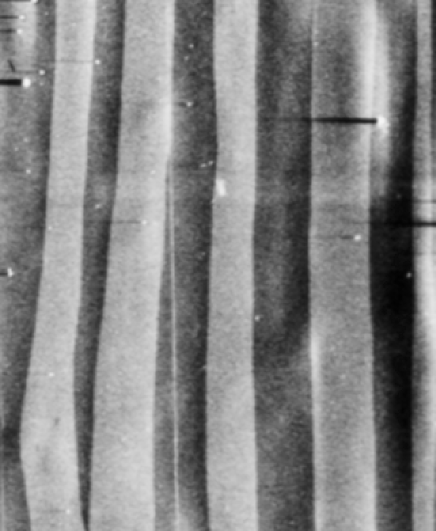
FIG. 1.: The domain structure of Fe₆₄Co₂₁B₁₅ amorphous alloy observed using the Kerr effect. The domains are separated by walls parallel to the magnetization. This is the typical structure observed in soft ferromagnetic materials.

II Experimental results

The experimental results on the Barkhausen effect form an enormous body of literature that spans almost the entire century [1, 2, 3, 4], but precise experimental results for the statistics of Barkhausen jumps have been reported only recently [5, 6, 7]. The distribution of Barkhausen jump sizes, measured at low driving rates, shows typically a power law behavior, but the scaling exponents reported in the literature span a wide range of values [29]. For this reason, it is important to carefully discuss the various experimental conditions, material properties and statistical uncertainties before direct comparison with a theory could be made.

Under well-defined experimental conditions the results show a remarkable degree of universality: the scaling exponents do not depend on the particular sample used [5, 6, 15, 29, 30, 31, 32]. The measurements are taken only in the central part of the hysteresis loop around the coercive field, where domain wall motion is dominant while domain nucleation and coherent spin rotations are negligible [15]. The typical domain structure observed in these conditions is reported in Fig. 1. Experiments were performed using a triangular waveform for the external field and different driving rates were employed.

The signal amplitude distribution, directly related to the domain wall velocity, decays as power law [5, 6, 15, 30]

$$P(v)\sim v^{-(1-c)}\exp(-v/v_{0}),$$ (1)

where $c$ is proportional to the field driving rate and $v_{0}$ is the value of the cutoff. The avalanche size $s$ (the area under the jump) and duration $T$ distributions also decay as power laws and are very well fitted by [5, 6, 29]

$$P(s)\sim s^{-\tau}f(s/s_{0})~{}~{}~{}~{}\tau=3/2-c/2,$$ (2)

$$P(T)\sim T^{-\alpha}g(T/T_{0})~{}~{}~{}~{}\alpha=2-c.$$ (3)

These laws have been tested for a variety of materials, such as amorphous (Co-base and Fe-base) [29, 33] and alloys (Fe-) [5, 6]. In Fig. 2, we report the size and duration distributions measured in an as cast Fe₂₁Co₆₄B₁₅ amorphous alloy for different field driving rates. The experiments have been performed using the setup described in Ref. [6]. The exponents agree perfectly with Eqs. (2-3).

The dependence of the exponents on the field driving rate [34] can explain the variability in the experimental values reported in literature, since many experiments were performed using a single linear driving rate [17] or a sinusoidal one. Moreover, one should also be aware that the properties of the noise and thus the scaling exponents and the cutoff can change considerably through the hysteresis loop [15, 35] when domain nucleation and coherent spin rotations become relevant.

To test the effect of the demagnetizing field, we perform experiments on strips of with different lengths of an as cast Fe₂₁Co₆₄B₁₅ amorphous alloy. The intensity of the demagnetizing field decreases for longer samples. We find that the cutoff of distributions scales as $s_{0}\sim 1/k$ and $T_{0}\sim 1/k^{1/2}$ (Fig. 3), where $k$ is proportional to the intensity of the demagnetizing field (see Section III). We obtain the same results controlling $k$ by changing the air gap between the sample and a magnetic joke. A complete account of these experiments will be deferred to a forthcoming publication.

The power spectrum $S(f)$ of the noise does not show in general such a marked robustness and is not described by a frequency-independent exponent: at low frequency $f$,

$$S(f)\sim f^{\psi},$$ (4)

where $\psi$ varies between $\psi\simeq 0.6$ in Fe-Si, to $\psi\simeq 1$ in amorphous alloys [29, 31, 32]. After a crossover frequency, that depends on $c$, it decays with an exponent varying between $-1.6$ and $-2$ [6, 7, 29, 31, 32]. When only a single domain wall is present the power spectrum was found to decay as $f^{-2}$ [2]. Moreover, it has been observed that the power spectrum amplitude scales linearly with $c$. From the point of view of applications, it is important to distinguish universal properties from material-dependent properties that could be relevant to characterize the sample.

In toroidal or frame geometries the demagnetizing field is practically absent and the magnetization process is quite different from in the previous case. The hysteresis loop, instead of showing a extended linear part with a stationary Barkhausen signal, displays a square form with a huge Barkhausen jump: the domain walls undergo a depinning transition as a function of the field. When the external field $H$ exceeds the coercive field $H_{c}$, the domain walls start to move with a velocity $v$ that typically scales linearly with the field

$$v\sim(H-H_{c}).$$ (5)

This law has been first observed about 50 years ago by Williams, Shockley and Kittel [36] in a single crystal Fe-Si frame, and later confirmed for a variety of other soft ferromagnetic materials [37]. Before the onset of collective domain wall motion, one observes a series of Barkhausen jumps of increasing amplitude [2], but to our knowledge a quantitative analysis in terms of scaling exponents has never been reported.

FIG. 2.: Distributions of Barkhausen jump sizes (a) and durations (b) measured in an as-cast Fe₂₁Co₆₄B₁₅ amorphous alloy for different driving rates. The lines are the fit with $\tau=3/2-c/2$ and $\alpha=2-c$. The distributions have been obtained recording $6\cdot 10^{5}$ avalanches.

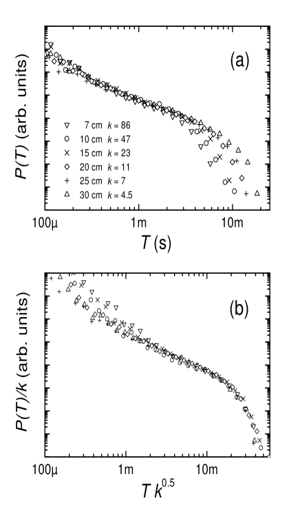
FIG. 3.: a) Distribution of Barkhausen jump durations measured in Fe₂₁Co₆₄B₁₅ amorphous alloy for different sample lengths. b) The data collapse shows that $T_{0}\sim k^{-0.5}$.

III Domain wall dynamics

The first thermodynamic theory of ferromagnetic domains is due to Landau and Lifshitz [38], who explained the presence of domains by energetic considerations. In a uniformly magnetized specimen, the discontinuity of the normal component of magnetization across the boundary of the sample creates a field that raises the total energy of the system. The creation of domains decreases this energetic contribution at the price of a higher cost in wall energy. One can obtain a rough estimate of the number of domains by simply balancing these two terms.

In order to describe accurately the magnetization process, it is necessary to analyze in detail the interactions present. In most ferromagnetic materials, due to the magnetocrystalline anisotropy or to the shape of the sample, the magnetization has preferred directions. In the simplest situation, there is a single easy axis of magnetization and the domains are separated by surfaces parallel to the magnetization, spanning the sample from end to end (see Fig. 1). The domain walls are in general flexible, since local inhomogeneities can impose distortions of the surface, which would be flat in a perfectly ordered system. In some particular geometry in which demagnetizing effects are minimized, it is even possible to obtain a single domain wall [2].

We study the dynamics of a single $180^{\circ}$ domain wall separating two regions with opposite saturation magnetizations, directed along the $x$ axis. If the surface has no overhangs, we can describe the position of the domain wall by a function $h(\vec{r},t)$ of space and time (see Fig. 4). The equation of motion for the wall is given by

$$\Gamma\frac{\partial h(\vec{r},t)}{\partial t}=-\frac{\delta E(\{h(\vec{r},t)\})}{\delta h(\vec{r},t)},$$ (6)

where $E(\{h(\vec{r},t)\})$ is the total energy functional for a given configuration of the surface and $\Gamma$ is an effective viscosity. The motion of the domain wall is overdamped, since eddy currents cancel inertial effects, and thermal effects are negligible.

We can split the energy into the sum of different contributions due to magnetostatic and dipolar fields, ferromagnetic and magnetocrystalline interactions, and disorder. In the following, we will express the energy in IS units.

A Magnetostatic fields

In the presence of an external field $\vec{H}$ along the easy axis of magnetization the magnetostatic energy of the system is given by

$$E_{m}=-2\mu_{0}HM_{s}\int d^{2}r\;h(\vec{r},t),$$ (7)

where $M_{s}$ is the saturation magnetization per unit volume.

Another contribution to the magnetostatic energy comes from the discontinuity of the normal component of the magnetization across the boundary of the sample. This generates an effective magnetic field, the so called demagnetizing field, that is opposed to the direction of the total magnetization. In some particular geometries (e.q. a uniformly magnetized ellipsoid) this field is constant along the sample. For a generic domain structure, an explicit expression for the demagnetizing field is often not available, but we expect in first approximation that the intensity of the demagnetizing field will be proportional to the total magnetization. Considering the field constant through the sample, its energy can be written as

$$E_{dm}=\frac{2\mu_{0}{\cal N}M_{s}^{2}}{V}\left(\int d^{2}r~{}h(\vec{r},t)\right)^{2},$$ (8)

where the demagnetizing factor $\cal{N}$ takes into account the geometry of the domain structure and the shape of the sample and $V$ is the sample volume. This term was also considered by Urbach et al. [17]. The demagnetizing effect can be avoided in suitable geometries, as in frame or toroidal specimens, but it is present in many common experimental situations.

B Dipolar interactions

An effect similar to the one discussed above takes place inside the sample, where the local curvature of the surface can in general give rise to discontinuities in the normal component of the magnetization. We treat this effect introducing a “magnetic charge” density, which for a domain wall separating two regions of magnetizations $\vec{M}_{1}$ and $\vec{M}_{2}$ is given by [39]

$$\sigma=(\vec{M}_{1}-\vec{M}_{2})\cdot\hat{n}$$ (9)

where $\hat{n}$ is normal to the surface. This charge is zero only when the magnetization is parallel to the wall. For small bending of the surface, we can express the charge as (see Fig. 4)

$$\sigma(\vec{r})=2M_{s}\cos\theta\simeq 2M_{s}\frac{\partial h(\vec{r},t)}{\partial x}$$ (10)

where $\theta$ is the local angle between the vector normal to the surface and the magnetization. The energy associated with a distribution of charges $\sigma$ is given by

$$E_{d}=\frac{\mu_{0}}{8\pi}\int d^{2}rd^{2}r^{\prime}\frac{\sigma(\vec{r})\sigma(\vec{r}^{\;\prime})}{|\vec{r}-\vec{r}^{\prime}|}.$$ (11)

Inserting the expression for $\sigma$ in Eq. (11) and integrating twice by parts, we obtain

$$E_{d}=\int d^{2}rd^{2}r^{\prime}h(\vec{r},t)K(\vec{r}-\vec{r}^{\;\prime})h(\vec{r}^{\prime},t)$$ (12)

where the non local kernel has the form [23]

$$K(\vec{r}-\vec{r}^{\;\prime})=\frac{\mu_{0}M_{s}^{2}}{2\pi|\vec{r}-\vec{r}^{\;\prime}|^{3}}\left(1+\frac{3(x-x^{\prime})^{2}}{|\vec{r}-\vec{r}^{\;\prime}|^{2}}\right).$$ (13)

The interaction is long range and anisotropic, as can be seen by considering the Fourier transform

$$K(p,q)=\frac{\mu_{0}M_{s}^{2}}{4\pi^{2}}\frac{p^{2}}{\sqrt{p^{2}+q^{2}}},$$ (14)

where $p$ and $q$ are the two components of the Fourier vector.

In the preceding derivation we have implicitly assumed that the medium is infinitely anisotropic, so that the magnetization never deviates from the easy axis. In practice, however, the magnetization will rotate slightly from the easy axis because of the field created by the surface charges. A local change in the magnetization produces additional volume charges whose density is given by

$$\rho(\vec{r})=\nabla\cdot\vec{M}.$$ (15)

Néel [12] has explicitly treated this effect obtaining an expression for the energy in the form of Eq. (12) with a modified kernel

$$\tilde{K}(p,q)\sim\frac{1}{\sqrt{Q}}\frac{p^{2}}{\sqrt{p^{2}+Qq^{2}}},$$ (16)

where $Q$ is a material dependent constant, whose value ranges from 5 to 10. This calculation shows that the qualitative features of the interaction do not change if a finite magnetocrystalline anisotropy is taken into account.

For the analysis we will perform later, it is important to generalize the kernel in any dimension. It is straightforward to show that for $d\geq 3$ the kernel scales as

$$K(q)\propto\frac{q_{\parallel}^{2}}{\sqrt{q_{\parallel}^{2}+q_{\perp}^{2}}},$$ (17)

where $q_{\parallel}$ and $\vec{q}_{\perp}$ are the components of $q$ parallel and perpendicular to the magnetization.

C Surface tension and disorder

The magnetocrystalline and exchange interactions are responsible for the microscopic energy associated with the domain wall. While a very sharp change of the spin orientation has a high cost in exchange energy, a very smooth rotation of the spins between two domains is prevented by the magnetocrystalline anisotropy. The balance between these two contributions determines the width of the domain wall and its surface energy. The total energy due to these contributions is proportional to the area of the domain wall

$$E_{dw}=\nu_{0}\int d^{2}r\sqrt{1+|\nabla h(\vec{r},t)|^{2}},$$ (18)

where $\nu_{0}$ is the surface tension. Expanding this term for small gradients we obtain

$$E_{dw}=\nu_{0}S_{dw}+\frac{\nu_{0}}{2}\int d^{2}r|\nabla h(\vec{r},t)|^{2},$$ (19)

where $S_{dw}$ is the domain wall area. This is the typical term associated with elastic interfaces.

The disorder present in the material in the form of non-magnetic impurities, lattice dislocations or residual stresses is the reason for the jumps in the magnetization curve and for its hysteretic behavior. We can treat the effect of the disorder by introducing a random potential $V(\vec{r},h)$, whose derivative gives the local pinning field $\eta(\vec{r},h)$ acting on the surface. We take this random field to be Gaussian-distributed and short range-correlated

$$\langle\eta(\vec{r},h)\eta(\vec{r}^{\;\prime},h^{\prime})\rangle=\delta^{2}(\vec{r}-\vec{r}^{\;\prime})R(h-h^{\prime})$$ (20)

where $R(x)$ decays very rapidly for large values of the argument.

D The equation of motion

Collecting all the energetic contributions, we obtain the equation of motion for the domain wall [28]. In order to avoid a cumbersome notation, we will absorb all the unnecessary factors in the definitions of the parameters. The equation then becomes

$$\frac{\partial h(\vec{r},t)}{\partial t}=H-k\bar{h}+\nu_{0}\nabla^{2}h(\vec{r},t)+$$ (21)

$$\int d^{2}r^{\prime}K(\vec{r}-\vec{r}^{\;\prime})(h(\vec{r}^{\;\prime})-h(\vec{r}))+\eta(\vec{r},h),$$ (22)

where the kernel $K$ is given by Eq. (13), $k\equiv 4\mu_{0}{\cal N}M_{s}^{2}$ [40], $\bar{h}\equiv\int d^{2}r^{\prime}h(\vec{r}^{\;\prime},t)/V$. Apart from the non-local kernel, this equation is similar to the equation proposed by Urbach et al., which on its turn reduces when $k=0$ to an elastic interface driven in quenched disorder. When the field is slowly increased, the demagnetizing field provides a restoring force that keeps the motion around the depinning transition. As we will show later, the non-local kernel changes the upper critical dimension, and hence the exponents, from the case of the elastic interface.

FIG. 4.: A domain wall separating two regions of opposite magnetization. The discontinuities of the normal component of the magnetization across the domain wall produce magnetic charges.

IV Mean-field theory and upper critical dimension

The mean-field theory provides a good qualitative description of the depinning transition [41, 42, 43]. We will consider first the case $k=0$ and $H$ constant, which correspond to a conventional depinning transition. We will discuss in section VI the case $k>0$, $H\propto t$. Here, we proceed as in Refs. [26, 44], considering an infinite ranged interaction kernel in the equation of motion. To this end, it is convenient to first discretize Eq. (22)

$$\frac{\partial h_{i}(t)}{\partial t}=H+\sum_{j}J_{ij}(h_{j}(t)-h_{i}(t))+\eta_{i}(h),$$ (23)

where $J_{ij}$ in Fourier space has the form

$$J(p,q)=\frac{Ap^{2}}{\sqrt{p^{2}+q^{2}}}+\nu_{0}(p^{2}+q^{2}),$$ (24)

where $A\equiv\mu_{0}M_{s}^{2}/4\pi^{2}$. The infinite range model is the same as in the elastic interface problem

$$\frac{\partial h_{i}(t)}{\partial t}=H+J(\bar{h}-h_{i}(t))+\eta_{i}(h),$$ (25)

where $\bar{h}\equiv\sum_{i}h_{i}/N$, $J\equiv A+\nu_{0}$ and $N$ is the system size. The mean-field behavior depends on the shape of the random potential: for cusped potentials one obtains that the velocity of the interface grows linearly for $H>H_{c}$

$$v\sim(H-H_{c}).$$ (26)

A complete mean-field analysis, including the form of response and correlation function, can be found in Refs. [42, 44].

To go beyond mean-field theory, Narayan and Fisher [26, 44] have devised a functional renormalization group scheme that allows one to obtain the value of the upper critical dimension and an estimate of the scaling exponents. Their method is based on an expansion around mean-field theory, using the formalism of Martin-Siggia-Rose. They construct a generating functional for the response and correlation functions, introducing an auxiliary field $\hat{h}(x,t)$,

$$Z=\int(dh)(d\hat{h})\exp\left\{i\int d^{d-1}x~{}dt\hat{h}F(h,\eta)\right\},$$ (27)

where

  

$$F(h,\eta)=\frac{\partial h(x,t)}{\partial t}-\nu_{0}\nabla^{2}h(x,t)-\int d^{d-1}x^{\prime}~{}K(x-x^{\prime})(h(x^{\prime},t)-h(x,t))-\eta(x,h)-H.$$ (28)

  

Following Ref. [26], we introduce a new field

$$\phi_{i}=\sum_{j}J_{ij}h_{j}$$ (29)

which represent of coarse grained version of $h$, and a corresponding auxiliary field $\hat{\phi}$. After averaging over the disorder one obtains an effective generating functional

$$\bar{Z}=\int(d\phi)(d\hat{\phi})\exp(\tilde{S}(\phi,\hat{\phi})),$$ (30)

whose saddle point value corresponds with the mean-field theory. Narayan and Fisher carried out an expansion around the saddle point to obtain the correction to the mean-field theory. In our problem everything works like in Ref. [26], the only difference being in the form of the interaction kernel ($J(q)\propto q^{2}$ in [26]). The effective action is in our case [45]

  

$$\tilde{S}=\int d^{d-1}x~{}dtH\hat{\phi}(x,t)+\int\frac{d^{d-1}q~{}d\omega}{(2\pi)^{d}}\hat{\phi}(-q,-\omega)(-i\omega+\frac{Aq_{\parallel}^{2}}{\sqrt{q_{\parallel}^{2}+q_{\perp}^{2}}}+\nu_{0}q^{2})\phi(q,\omega)$$ (31)

$$-\frac{1}{2}\int d^{d-1}x~{}dtdt^{\prime}\hat{\phi}(x,t)C(vt-vt^{\prime}+\phi(x,t)-\phi(x,t^{\prime}))\phi(x,t),$$ (32)

where the function $C(x)$ is the mean-field correlation function. Other terms resulting from the expansion around the saddle point can be seen to be irrelevant.

To obtain the upper critical dimension, we rescale space and time $x=bx^{\prime}$, $t=b^{z}t^{\prime}$, $\phi=b^{\zeta}\phi^{\prime}$, $\hat{\phi}=b^{\theta-d+1}\hat{\phi}^{\prime}$ and $H=b^{-1/\nu}H^{\prime}$, requiring that the Gaussian part of the action remains invariant. Simple power counting gives

$$z=1~{}~{}~{}\zeta=\frac{3-d}{2}~{}~{}~{}\theta=\frac{d-3}{2}~{}~{}~{}\nu=\frac{2}{d-1}.$$ (33)

For $d>3$ all non linearities decay to zero at large lengthscale and the theory is Gaussian, while for $d<3$ an infinite set of non linear terms becomes relevant. The upper critical dimension for this problem is therefore $d_{c}=3$. This result differs from the one obtained for elastic interfaces, for which $d_{c}=5$, but agrees with the result for contact line depinning [46]. The similarity between the two problems lies in the non-local kernel that scales linearly with the momentum at long length scales.

In order to apply these results to the experiments we have to make sure that the linear part of the kernel dominates on the length scales of interest. Long-range effects become relevant for length scales larger than $L\sim 2\pi\nu_{0}/\mu_{0}M_{s}^{2}$. In typical ferromagnets, $\mu_{0}M_{s}\sim 1$ and $\nu_{0}\sim 10^{-3}$ (in IS units) (see page 713 of [11]). This implies $L~{}\sim 10^{-9}\div 10^{-8}\mbox{ m}$, which is of the order of the domain wall thickness. From this calculation we conclude that the effect of the surface tension can be neglected with respect to the long-range kernel.

Above the upper critical dimension mean-field results are valid, while for $d=d_{c}$ we expect logarithmic corrections. To obtain the value of the exponents below the upper critical dimension one should perform a functional renormalization group along the lines of Refs. [25, 26, 44]. This has been done in Ref. [46] in the case of a kernel scaling linearly in momentum space. However, in many experimental situations the magnetization is perpendicular to the plane of the film and this analysis does not apply. The issues of Barkhausen effect and domain growth in thin films deserve further investigations that are beyond the scope of this paper.

V Critical exponents for constant applied field

In this section we derive scaling relations between the exponents that characterize the depinning transition. When the external field is increased monotonically and adiabatically the interface moves in avalanches of increasing size. The exponents describing avalanche distributions can be compared with experiments on the Barkhausen effect. We have to keep in mind that most experiments are performed with a non zero applied field rate in presence of demagnetizing field. We expect however that the distributions at $H=H_{c}$ should scale as in the case $c\to 0$ and $k\to 0$.

The avalanche size distribution close to the depinning transition scales as

$$P(s)\sim s^{-\tau}f(s/s_{0}),$$ (34)

where the cutoff scales as $s_{0}\sim(H-H_{c})^{-1/\sigma}$ and is related to the correlation length $\xi$ by

$$s_{0}\sim\xi^{d-1+\zeta},$$ (35)

where $\zeta$ is the roughness exponent (Fig. 5). The correlation length diverges at the depinning transition as

$$\xi\sim(H-H_{c})^{-\nu},$$ (36)

which implies

$$\frac{1}{\sigma}=\nu(d-1+\zeta).$$ (37)

The average avalanche size also diverges at the transition

$$\langle s\rangle\sim(H-H_{c})^{-\gamma},$$ (38)

where $\gamma$ is related to $\tau$ and $\sigma$ by

$$\gamma=\frac{(2-\tau)}{\sigma}.$$ (39)

An additional scaling relation can be obtained considering the susceptibility [26] which is proportional to $\langle s\rangle$ and scales as

$$\frac{d\langle h\rangle}{dH}\sim(H-H_{c})^{-(1+\nu\zeta)}.$$ (40)

This relation together with Eq. 39 implies

$$\tau=2-\frac{1+\nu\zeta}{\nu(d-1+\zeta)}.$$ (41)

The other exponent relevant for the Barkhausen effect describes the distribution of avalanche durations

$$P(T)\sim T^{-\alpha}g(T/T_{0}),$$ (42)

where the cutoff diverges at the transition as $T_{0}\sim(H-H_{c})^{-1/\tilde{\sigma}}$. From Eq. (36) and the relation $T_{0}\sim\xi^{z}$ we obtain $\tilde{\sigma}=1/z\nu$ and

$$\alpha=1+\frac{\nu(d-1)-1}{z\nu}.$$ (43)

We note that all relations (35-43) are valid also for other interface problems provided $d\leq d_{c}$.

For our case in $d=3$, which corresponds to the upper critical dimension, we have $\zeta=0$, $z=1$ and $\nu=1$, that inserted in the previous expressions give $\tau=3/2$ and $\alpha=2$. These exponents agree very well with experimental results in the limit of adiabatic driving ($c\to 0$). Moreover, we obtain that the average avalanche size scales with the duration as

$$\langle S(T)\rangle\sim T^{2}$$ (44)

which has been recorded experimentally in Ref. [6]. It is interesting to compare these results with the exponents obtained for three dimensional elastic interfaces. In that case the $\epsilon$-expansion gives $\zeta=2/3$, $z=14/9$ and $\nu=3/4$ which imply $\tau=1.25$ and $\alpha=1.43$ [25, 26, 47]. Simulations give slightly different values, $\tau\simeq 1.3$ and $\alpha\simeq 1.5$ [47]. In any case, the values are significantly lower than the experimental results.

When the experiment is performed in absence of demagnetizing fields, as for example in frame geometries, it is possible in principle to measure the exponent close to the depinning transition. In this regard, several experiments, discussed in section II, support the mean-field prediction $v\sim(H-H_{c})$. Vergne et al. [2] have observed the growth of the size of the Barkhausen jumps as the field is increased. From a measurement of this kind it should be possible to obtain an estimate of the exponent $\gamma$. We believe that similar experiments are crucial to confirm the presence of a depinning transition.

Finally, we discuss the properties of the power spectrum of the velocity signal. A similar analysis, in the context of flux line depinning, is reported by Tang et al. [48]. The height autocorrelation function scales as

$$\langle h(\vec{r},t)h(\vec{r}~{}^{\prime},t^{\prime})\rangle\sim|t-t^{\prime}|^{2\zeta/z}f(|\vec{r}-\vec{r}~{}^{\prime}|/|t-t^{\prime}|^{1/z}).$$ (45)

The scaling of the velocity autocorrelation function is obtained deriving Eq. (45) with respect to time, which gives a power law decay with exponent $2(\zeta/z-1)$. The power spectrum of the velocity signal at some fixed space location $\vec{r}$ scales therefore like

$$S_{v}(\omega)\sim\omega^{\psi};~{}~{}~{}~{}~{}~{}~{}\psi=1-2\zeta/z.$$ (46)

When the velocity is averaged over the whole system we expect instead

$$S_{\bar{v}}(\omega)\sim\omega^{\tilde{\psi}};~{}~{}~{}~{}~{}~{}~{}\tilde{\psi}=1-(2\zeta+1)/z.$$ (47)

In mean-field theory $\zeta=0$, which implies $\psi=1$ and $\tilde{\psi}=0$. It is interesting to compare these results with three dimensional elastic interfaces for which $\psi\simeq 0.1$ and $\tilde{\psi}=-0.6$ [49]. The direct comparison of these values with experimental results is not straightforward due to the complexity of the measured spectra. We expect the exponents derived from the depinning transition to describe the low-frequency part of the power spectrum, while for high frequencies we observe a $1/f^{2}$ decay [48]. For low frequencies experiments find exponents ranging from $0.5$ to $1$. This range of value lies between the predictions for $\tilde{\psi}$ and $\psi$. We considered the possibility of a crossover effect, since in the typical experiment the pick-up coil is much smaller than the system size. Depending on the domain structure and the coil size the experimental exponents could lie anywhere between the averaged and non-averaged result. We tested experimentally this hypothesis, varying the size of the pick-up coil but we noticed no changes in the low frequency part of the spectrum. To obtain a complete explanation of the power spectrum, we should probably take into account the presence of many interacting domain walls and magnetic after effect.

FIG. 5.: The interface moves between two pinned configuration in an avalanche of size $s\sim l^{d-1+\zeta}$

VI Driving rate and demagnetizing field

In this section we study the effect of the driving rate and the demagnetizing field on the dynamics of the model. We study here the infinite range model, that in $d=3$ should have the same critical behavior of the long range model, but it is much simpler to analyze.

As discussed in [17], the demagnetizing field has the effect of keeping the interface close to the depinning transition. We will show that the intensity of the demagnetizing field is a relevant parameter controlling the avalanche characteristic length. Criticality is reached only when this parameter is vanishingly small. A finite driving rate changes continuously the critical exponents, as in the ABBM model [15]. We will numerically show that the infinite range model reproduces the results of the ABBM model and we will present an argument explaining the reason for this behavior. This observation explains the success of the ABBM model in fitting experimental data.

The dynamics of the infinite range model is described by the following equation

$$\frac{\partial h_{i}(t)}{\partial t}=H(t)-k\bar{h}+J(\bar{h}-h_{i}(t))+\eta_{i}(h),$$ (48)

where the external field $H(t)$ is increased at constant rate and the demagnetizing field $H_{d}=-k\bar{h}$ has been included.

To show the equivalence with the ABBM model, we sum over $i$ both sides of Eq. (48) and obtain an equation for the total magnetization $m$

$$\frac{dm}{dt}=\tilde{c}t-km+\sum_{i=1}^{N}\eta_{i}(h),$$ (49)

where the time dependence of the field is now explicit. This equation has the same form of the ABBM model provided we can interpret $\sum_{i}\eta_{i}$ as an effective pinning $W(m)$, with Brownian correlations. When the interface moves between two pinned configuration $W$ changes as

$$W(m^{\prime})-W(m)=\sum_{i=1}^{n}\Delta\eta_{i},$$ (50)

where the sum is restricted to the $n$ sites that have effectively moved (i.e. their disorder is changed). The total number of such sites scales as $n\sim l^{d-1}$ and in mean-field theory is proportional to the avalanche size $s=|m^{\prime}-m|$ (since $s\sim l^{d-1+\zeta}$ and $\zeta=0$). Assuming that the $\Delta\eta_{i}$ are uncorrelated and have random signs, we obtain a Brownian effective pinning field [50]

$$\langle|W(m^{\prime})-W(m)|^{2}\rangle=D|m^{\prime}-m|,$$ (51)

where $D$ quantifies the fluctuation in $W$. The Brownian pinning field, observed experimentally in SiFe alloys and used in the ABBM model to describe the motion of the domain wall, is not due to a long-range correlated disorder present in the material. It is instead the result of the collective motion of the interface and therefore represents only an effective description of the disorder.

The main predictions of the ABBM model can be obtained as follows. We derive Eq. (49) with respect to time and define $v\equiv dm/dt$

$$\frac{dv}{dt}=\tilde{c}-kv+vf(m),$$ (52)

where $f(m)\equiv dW/dm$ is an uncorrelated random field. Expressing Eq. 52 as a function of $v$ and $m$ only

$$\frac{dv}{dm}=\frac{\tilde{c}}{v}-k+f(m),$$ (53)

we obtain a Langevin equation for a random walk in a confining potential, given by $E(v)=kv-\tilde{c}\log(v)$. In the limit of large $m$, $v$ is given by the Boltzmann distribution

$$P(v,m\to\infty)\sim\exp(-E(v)/D)=v^{c}\exp(-kv/D),$$ (54)

where $c\equiv\tilde{c}/D$.

The distribution in the time domain is obtained by a simple transformation and it is given by [15]

$$P(v)\equiv P(v,t\to\infty)=\frac{k^{c}v^{c-1}exp(-kv/D)}{D^{c}\Gamma(c)}.$$ (55)

Eq. (55) predicts that the domain wall moves at constant average velocity $\langle v\rangle=\tilde{c}/k$. The relative fluctuations of the velocity diverge in the adiabatic limit $c\to 0$

$$\frac{\sqrt{\langle v^{2}\rangle-\langle v\rangle^{2}}}{\langle v\rangle}=\sqrt{\frac{1}{c}}.$$ (56)

This divergence is due to the singularity at low velocities of Eq. (55) and reflects the presence of a depinning transition. For $c<1$ the velocity distribution is a power law with an upper cutoff that diverges as $k\to 0$. In this regime, the domain wall moves in avalanches whose size and durations are also distributed as power laws. The avalanche size distribution is directly related to the distribution of first return times of a random walk in the confining potential $E(v)$. Using scaling relations, it has been shown [6] that the avalanche exponents scale as a function of $c$ as

$$\tau=3/2-c/2~{}~{}~{}~{}~{}\alpha=2-c,$$ (57)

in agreement with experimental results.

The scaling of the cutoff of the avalanche distributions can be obtained as follows. For $k=0$, the cutoff in the size distribution scales with $H$ as $s_{0}\sim(H-H_{c})^{-1/\sigma}$, and similarly for the distribution of durations. When $k>0$, the interface experience an effective field $H-k\bar{h}$ which keeps it on average below the depinning transition. We assume that the distance from the critical point $H_{c}$ is of the order of

$$\Delta H=H-H_{c}\sim k\Delta\bar{h},$$ (58)

where $\Delta\bar{h}$ is the average variation of the height corresponding to a variation $\Delta H$ in the field. Since $\Delta\bar{h}\sim\langle s\rangle\Delta H$, the average avalanche size scales as $1/k$, which implies

$$s_{0}\sim k^{-2}.$$ (59)

Using similar arguments we can also show that the cutoff of avalanche durations scales as $T_{0}\sim k^{-1}$ in mean-field theory. These results do not agree with the experiments presented in section II. We will show in the next section that they are a peculiarity of mean-field theory and are not obeyed by the equation in $d=3$.

Finally, we note that avalanches are observed only for small driving rates ($c<1$). For $c>1$ the motion is smoother with fluctuations that decrease as $c$ increases, in agreement with experiments [15].

VII Simulations

A The infinite-range model

We simulate the infinite-range model in order to confirm its equivalence with the ABBM model. We first integrate numerically Eq. (48), using the Runge-Kutta method and a random potential composed by parabolas with cusp singularities [44, 26]. We study the velocity signal as a function of the driving rate $\tilde{c}$, and find that on increasing $\tilde{c}$, the dynamics crosses over from avalanche dominated motion at low $\tilde{c}$ to a smoother motion at larger $\tilde{c}$ (see Fig. 6). We are able to integrate the model only for relatively small values of $N$; therefore it is not possible to observe the scaling of avalanche distributions, which appear to be dominated by finite size effects.

We then introduce an automaton version of the infinite range model, which can be simulated for much larger system sizes, and study it for different values of $c$ and $k$. From the results of the ABBM model, we expect that the velocity distribution is described by Eq. (55). In the limit $c\to 0$, the cutoff in the exponential is $v_{0}=k/D$. We extract $v_{0}$ from the velocity distribution (see Fig. 7a) and we plot it for different values of $k$ in Fig. 7b. As expected, we observe a linear decay and we find a value $1/D=1.3\pm 0.1$. We then compute the avalanche size and duration distribution in the $c\to 0$ limit as a function of $k$. The data collapse perfectly (see Figs. 8 and 9) using the scaling forms predicted in the previous section

$$P(s,k)\sim s^{-3/2}f(sk^{2}),$$ (60)

$$P(T,k)\sim T^{-2}g(Tk).$$ (61)

Next, we simulate the model as a function of $\tilde{c}$ and find scaling exponents that depend linearly on the driving rate. The avalanche size distribution shows a power law for more than four decades. Therefore, it provides a reliable estimate of $c$, using the relation $\tau=3/2-c/2$. We compute $\tau$ from the distribution as function of $\tilde{c}$ and observe a linear behavior $\tau=3/2-\tilde{c}/(2D)$, with $1/D\simeq 1.2$, which is consistent with the scaling of the cutoff of the velocity distribution (Fig. 7b). The value of $c$ obtained above can then used to fit the velocity and avalanche duration distributions and the results are consistent with the theory (see Figs. 10 and 11).

Finally, we compute the power spectrum for different values of $c$. We observe a $1/f^{2}$ decay at large frequency and a constant part at low frequencies. The crossover point scales linearly with $c$ as in experiments [15].

FIG. 6.: The velocity of the interface as a function of time, for different values of $\tilde{c}$. The data have been obtained integrating the equation of motion with cusped potential for $N=256$.

FIG. 7.: (a) The distribution of velocities in the infinite-range automaton model as a function of $k$ for $N=32696$, $c=0$. (b) The scaling of the $1/v_{0}$ cutoff with $k$. The line is a fit with slope $1/D\simeq 1.3$.

FIG. 8.: (a) The distribution of avalanche sizes in the infinite-range automaton model as a function of $k$ for $N=32696$, $c=0$. A line corresponding to $\tau=3/2$ is plotted for comparison. (b) The corresponding plot, using scaled variables, showing excellent data collapse.

FIG. 9.: (a) The distribution of avalanche durations in the infinite-range automaton model as a function of $k$ for $N=32696$, $c=0$. A line corresponding to $\alpha=2$ is plotted for comparison. (b) The corresponding plot, using scaled variables, showing excellent data collapse.

FIG. 10.: The distribution of velocities in the infinite-range automaton model as a function of $c$ for $N=32696$, $k=0.0075$. The lines are the theoretical predictions $1-c$.

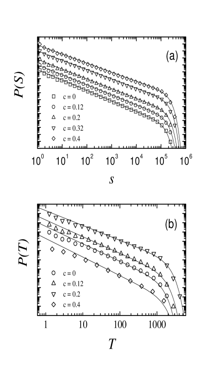
FIG. 11.: (a)The distribution of avalanche sizes in the infinite-range automaton model for different driving rates for $N=32696$, $k=0.0075$. The fit of the power-law part yields $\tau=3/2-c/2$, with $c=\tilde{c}/D$ and $1/D\simeq 1.2$. (b) The corresponding distribution of avalanche durations. The power-law part is fit with an exponent $\alpha=2-c$.

B The long-range model

A numerical integration of Eq. (22) poses serious numerical problems due to the presence of long range non-local kernel. Therefore, we study an automaton version of the model, which should belong to the same universality class. In the automaton model the height is discretized and the local velocity can assume only the values $v=0,1$. For each configuration of the system, we compute the local force according to Eq. (22). Periodic boundary conditions are imposed on the lattice and therefore we must sum the non-local kernel over the images as discussed in Ref. [51]. To model the disorder, we associate to each site on the interface a random number chosen from a Gaussian distribution.

When the local force on a site is larger than zero, the corresponding height is increased by one unit and we chose a new value for the disorder. Care must be taken in choosing the values of the parameters, in order to avoid instabilities present in the discretization of the kernel [52].

We consider first the case $k=0$ to confirm the predictions about the upper critical dimension. We increase the external filed adiabatically up to $H_{c}$ (i.e. when the interface is pinned we increase the external field until the most unstable site reaches the threshold for movement), and we compute the integrated avalanche size distribution. This distribution scales as

$$P_{int}(s)=\int_{0}^{H_{c}}dHP(s,H)\sim s^{-(\tau+\sigma)},$$ (62)

which yields a $s^{-2}$ decay in mean-field theory. Similarly, for the integrated duration distribution we find a $T^{-3}$ decay. The simulation results confirm the predictions of the theory (see Fig. 12).

Next, we study the model in the adiabatic limit ($c\to 0$) as a function of $k$. We compute the distribution of velocities (Fig. 13) and avalanches sizes (Fig. 14 ) and durations (Fig. 15 ) as a function of the demagnetizing field $k$. The scaling exponents are in agreement with the results of the depinning transition in the mean-field, $\tau=3/2$ and $\alpha=2$.

However, the scaling of the cutoff of the distributions does not agree with the predictions of the ABBM model. We find instead $s_{0}\sim k^{-1}$ and $T_{0}\sim k^{-1/2}$. This behavior persists in simulations performed at $c>0$, where the exponent $\tau$ and $\alpha$ still scale with $c$ as in the ABBM model. To obtain a good data collapse, the scaling functions in Eqs. (60) and (61) have to be replaced by

$$P(s,k)\sim s^{-3/2}g_{1}(sk),$$ (63)

$$P(T,k)\sim T^{-2}g_{2}(Tk^{1/2}),$$ (64)

which are the scaling forms obtained experimentally (see section II).

The precise reason for these results is still not completely clear. Recent simulations of a model similar to ours, studied in the context of dry friction, suggest that the effective pinning field for the long-range model is not Brownian [53]. In Ref. [53] the cut-off of the distributions was related to the shape of the force distribution, but it is not clear if this analysis can be applied directly to our case, due to the different driving mechanism employed in Ref. [53].

FIG. 12.: The integrated avalanche size distribution in the long-range automaton model for $k=0$ and $L=61$. A line with slope $-2$ is plotted for reference.

FIG. 13.: The velocity distribution in the long-range automaton model for $c=0$ and $L=61$. A line with slope $-1$ is reported for reference. In the inset we show the linear-log plot of the same distribution in order to show the exponential cutoff.

FIG. 14.: a) The avalanche size distribution for $c=0$ as a function of $k$ for the long-range automaton model with $L=61$. A line with slope $-3/2$ is reported for reference. b) The corresponding plot, using scaled variables, showing excellent data collapse.

FIG. 15.: a) The avalanche duration distribution as a function of $k$ in the long-range automaton model for $c=0$ and $L=61$. A line with slope $-2$ is reported for reference. b) The corresponding plot, using scaled variables, showing excellent data collapse.

VIII Discussion

In this paper we have studied the dynamics of a flexible domain wall as it moves through a disordered medium. We have derived an equation of motion taking into account the effect of different energetic contributions. A crucial role is played by dipolar interactions that give rise to a demagnetizing field and to a long-range interaction kernel. In absence of demagnetizing field, the domain wall shows a depinning transition as a function of the field. The long-range interaction kernel set the upper critical dimension to $d_{c}=3$, so that mean-field scaling should describe the experiments on the Barkhausen effect.

The predictions of the present theory compare well with the distribution of Barkhausen jump durations and sizes and with the velocity distribution. In particular, we discuss the linear dependence of the exponents on the field driving rate [5, 6, 31, 32] and the scaling of the cutoff with the demagnetizing field. The agreement between theory and experiments is in both cases quantitative. In toroidal geometries, when the demagnetizing field is zero, we predict a linear dependence of the domain wall velocity on the applied field, in agreement with several experiments on soft ferromagnetic materials [37].

We show that the phenomenological model introduced by ABBM [15] is equivalent to the infinite-range domain wall. The Brownian correlated random pinning field used in [15] and experimentally observed in [2] is shown to arise in the effective description of the motion of center of mass of the domain wall. This result clarifies the origin of the correlated disorder which could not be explained as a simple result of the correlations between the impurities [16]. While the infinite range model, and therefore the ABBM model, quantitatively explains many features of the Barkhausen effect, it does not give the correct dependence on the demagnetizing field, which is instead provided by the complete three-dimensional description.

The power spectrum of the Barkhausen noise does not show a marked universality and therefore can not be completely explained by our approach. In particular, we obtain a $1/f^{2}$ decay at large frequencies, which has only been observed in experiments with a single domain wall [2]. Other experimental results seem to suggest that the exponent changes when the number of domain walls increases [6, 31, 32]. Moreover, magnetic after-effect [11] and flux propagation could also affect the results. To obtain a quantitative explanations of these results, one should analyze the dynamics of many coupled domain walls.

The presence of many domain walls should affect the power spectrum, but not the avalanche distributions. When a domain wall starts to move, the demagnetizing field increases, creating a larger pinning force on the other walls. Therefore, on short time scales the interactions between the walls are irrelevant. For this reason, the avalanche distribution for a single domain wall agrees with experiments performed with many domain walls.

With our approach we can address several other issues raised in the literature about the Barkhausen effect. The partial reproducibility of the Barkhausen signal observed in recent experiments [16, 54, 55] is explained by the quenched nature of the disorder. Pushing the wall back and forth through the same disordered region of the sample results in the same signal. Deviations from this ideal behavior can be expected due to small variations on the initial conditions, thermal effects or differences in the driving rate. To understand these features it is crucial to consider a flexible domain wall instead of a rigid wall [15], for which always perfect reproducibility is expected.

The recent theoretical revival in the study of the Barkhausen effect is mostly due to the claim of Ref. [4] that this phenomenon is an example of self-organized criticality (SOC) [56]. This claim was challanged in Ref. [22] which, based on the results obtained for the RFIM, concluded that scaling in Barkhausen effect is due to the presence of a “plain old” critical point. The question concerns the origin of the cutoff in the power-law distributions. According to the analysis of Refs. [20, 21, 22], the cutoff would be determined by the variance of the random-field distribution. As far as we know, no experimental evidence of a critical point of this kind has been reported in the literature.

We have experimentally observed that the cutoff of the distributions is determined by the demagnetizing field, in agreement with our theoretical analysis. In our model, the critical point is reached only by fine tuning to zero the driving rate and the demagnetizing field, performing the limits $c\to 0$ and $k\to 0$ in the given order. This result implies that the idea of a critical point without tuning parameters does not apply to the Barkhausen effect. It is interesting to remark, however, that the picture revealed by our approach is similar to the one presented in Ref. [57], where it was shown that criticality in SOC models arise by the fine tuning to zero of the driving rate and other parameters. In light of these results, one should review the definition of SOC [57], dropping the notion of “criticality without fine-tuning”. In this restricted sense, the Barkhausen effect can be considered as a good example of SOC.

The present approach to the Barkhausen effect, based on the depinning of a ferromagnetic domain wall, applies to three dimensional soft ferromagnetic materials, which are frequently used in experimental studies of the Barkhausen effect. For hard ferromagnet and rare earth materials, where strong local anisotropies prevent the formation of straight domain walls, a different approach is needed. Disordered spin models like those presented in Refs. [20, 21, 22] seem more appropriate. We did not discuss here the issue of domain nucleation and growth in thin films (two dimensional ferromagnets). Depending on the material properties and the sample geometry, the domain walls are either fractal or self-affine as in our case. In the second case, we expect that the framework of the depinning transition could be relevant.

REFERENCES

- [1] H. Barkhausen, Z. Phys. 20, 401 (1919).
- [2] R. Vergne, J. C. Cotillard, and J. L. Porteseil, Rev. Phys. Appl. 16, 449 (1981).
- [3] H. Bittel, IEEE Trans. Magn. 5, 359 (1969); J. A. Baldwin and G. M. Pickles, J. Appl. Phys. 43, 1263 (1972); W. Grosse-Nobis, J. Magn. Magn. Mat. 4 247 (1977); U. Lieneweg and W. Grosse-Nobis, Int. J. Magnetism, 3, 11 (1972). K. P. O’Brien and M. B. Weissmann, Phys. Rev. E 50, 3446 (1994).
- [4] P. J. Cote and L. V. Meisel, Phys. Rev. Lett. 67, 1334 (1991); Phys. Rev. B 46, 10822 (1992).
- [5] G. Bertotti, G. Durin, and A. Magni, J. Appl. Phys. 75, 5490 (1994).
- [6] G. Durin, G. Bertotti, and A. Magni, Fractals 3, 351 (1995).
- [7] D. Spasojević, S. Bukvić, S. Milosević, and H. E. Stanley, Phys. Rev. E 54, 2531 (1996).
- [8] S. Field, J. Witt, F. Nori, and X. Ling, Phys. Rev. Lett. 74, 1206 (1995).
- [9] A. Petri, G. Paparo, A. Vespignani, A. Alippi, and M. Costantini, Phys. Rev. Lett. 73, 3423 (1994); S. Zapperi, A. Vespignani, and H. E. Stanley, Nature 388, 658 (1997).
- [10] G. Gutenberg and C. F. Richter, Ann. Geophys 9, 1 (1956).
- [11] A. Herpin, Théorie du magnetisme (Presse Universitaires de France, Paris 1968).
- [12] L. Néel, Ann. Univ. Grenoble 22, 299 (1946).
- [13] L. Néel, Cah. Phys. 12, 1 (1942); ibid. 13, 1 (1943).
- [14] J. A. Baldwin and G. J. Culler, J. Appl. Phys. 40, 2828 (1969); J. A. Baldwin, ibid. 42, 1063 (1971).
- [15] B. Alessandro, C. Beatrice, G. Bertotti, and A. Montorsi J. Appl. Phys. 68, 2901 (1990); ibid. 68, 2908 (1990).
- [16] J. R. Petta, M. B. Weissman, and K. P. O’Brien, Phys. Rev. E 54, R1029 (1996).
- [17] J. S. Urbach, R. C. Madison, and J. T. Markert, Phys. Rev. Lett. 75, 276 (1995).
- [18] O. Narayan, Phys. Rev. Lett. 77, 3855 (1996).
- [19] A. L. Barabasi and H. E. Stanley, Fractals Concepts in Surface Growth (Cambridge University Press, Cambridge, 1995)
- [20] J. P. Sethna, K. Dahmen, S. Karta, J. A. Krumhansl, and J. D. Shore, Phys. Rev. Lett. 70, 3347 (1993).
- [21] K. Dahmen and J. P. Sethna, Phys. Rev. Lett. 71, 3222 (1993); Phys. Rev. B 53, 14872 (1996). K. Dahmen, Ph. D. thesis, Cornell University (1995).
- [22] O. Perkovic, K. Dahmen, and J. P. Sethna, Phys. Rev. Lett. 75, 4528 (1995).
- [23] H. R. Hilzinger and H. Kronmüller, J. Magn. Magn. Mat 2, 11 (1976); H. R. Hilzinger, Phil. Magazine, 36, 225 (1977).
- [24] J. P. Bouchaud and A. Georges, Phys. Rev. Lett. 68, 3908 (1992).
- [25] T. Nattermann, S. Stepanow, L. H. Tang, and H. Leschhorn J. Phys. II (France) 2, 1483 (1992).
- [26] O. Narayan and D. S. Fisher, Phys. Rev. B 48, 7030 (1993).
- [27] M. Mezard and G. Parisi, J. Phys. (France) I 1, 809 (1991); L. Balents, J. P. Bouchaud, and M. Mezard ibid. 6, 1007 (1996).
- [28] P. Cizeau, S. Zapperi, G. Durin, and H. E. Stanley, Phys. Rev. Lett. 79, 4669 (1997).
- [29] G. Durin, in Proc. of the 14th Int. Conf. on Noise in Physical Systems and 1/f Fluctuations, C. Claeys and E. Simoen eds. (World Scientific, Singapore, 1997).
- [30] G. Bertotti, F. Fiorillo and A. Montorsi, J. Appl. Phys. 67, 5574 (1990).
- [31] G. Durin, C. Beatrice, and G. Bertotti, IEEE Trans. Magn. 30, 464 (1994).
- [32] G. Durin, A. Magni, and G. Bertotti, J. Magn. Magn. Mat. 140, 1835 (1994).
- [33] G. Durin, P. Cizeau, S. Zapperi, and H. E. Stanley, E. J. Phys. Appl. Phys. XXX, XXX (1998).
- [34] A similar dependence of the avalanche exponents on the external driving rate has also been observed in friction experiments. S. Ciliberto and C. Laroche, J. Phys. I (France) 4, 223 (1994).
- [35] D. Spasojević, S. Bukvić, S. Milosević, and I. Savić, unpublished.
- [36] H.J. Williams, W. Shockley, and C. Kittel Phys. Rev. 80, 1090 (1950).
- [37] J. K. Galt, Bell. Syst. Tech. J. 33 1023 (1954); C. P. Bean, and D. S. Rodbell, J. Appl. Phys. 26, 124 (1955); D. S. Rodbell and C. P. Bean, Phys. Rev. 103, 886 (1956).
- [38] L. Landau and E. Lifschitz, Phys. Z. 8, 153 (1935).
- [39] J. D. Jackson, Classical Electrodynamics (Wiley, New York, 1962)
- [40] Unfortunately, in Ref. [28] we used a slightly different notation for the demagnetizing field which was not correct dimensionally. The of Ref. [28] is called here .
- [41] D. S. Fisher, Phys. Rev. B 31, 1396 (1985).
- [42] H. Leschhorn, J. Phys. A 25, L555 (1992).
- [43] J. Koplik and H Levine, Phys. Rev. B 32, 280 (1985).
- [44] O. Narayan and D. S. Fisher, Phys. Rev. Lett. 68, 3615 (1992); Phys. Rev. B 46, 11520 (1992).
- [45] As in Ref. [26] we have subtracted from and their value at the saddle point.
- [46] D. Ertas and M. Kardar, Phys. Rev. E 49, R2532 (1994).
- [47] H. Leschhorn, T. Nattermann, S. Stepanow, and L. H. Tang, Ann. Physik 6, 1 (1997).
- [48] C. Tang, S. Feng, and L. Golubovic, Phys. Rev. Lett. 72, 1264 (1994).
- [49] Narayan [18] reported for a two-dimensional elastic interface, which he compares with three-dimensional experimental results.
- [50] This result can be also demonstrated rigorously. J. P. Bouchaud, private communication.
- [51] A. F. Bower, and M. Ortiz, J. Mech. Phys. Solids 38, 443 (1990).
- [52] J. Schmittbuhl, S. Roux, J.P. Villotte, and K. J. Maloy, Phys. Rev. Lett. 74, 1787 (1995).
- [53] A. Tanguy, M. Gounelle, and S. Roux, preprint; A. Tanguy, Ph. D. thesis, Université de Paris VII (1998).
- [54] J. S. Urbach, R. C. Madison, and J. T. Markert, Phys. Rev. Lett. 75, 4694 (1995)
- [55] J. R. Petta, M. B. Weissman, and G. Durin, Phys. Rev. E 56, 2776 (1997).
- [56] P. Bak, C. Tang, and K. Wiesenfeld, Phys. Rev. Lett. 59, 381 (1987).
- [57] A. Vespignani, and S. Zapperi, Phys. Rev. Lett. 78, 4793 (1997); Phys. Rev. E 57, xxx (1998); R. Dickman, A. Vespignani, and S. Zapperi, Phys. Rev. E 57, xxx (1998).