Studies of the phase diagram of randomly interacting fermionic systems

We present details of the phase diagrams of fermionic systems with random and frustrated interactions emphasizing the important role of the chemical potential $\mu$. The insulating fermionic Ising spin glass model is shown to reveal different entangled magnetic instabilities and phase transitions. We review tricritical phenomena related to the strong correspondence between charge and spin fluctuations and controlled by quantum statistics. A comparison with the diluted Sherrington–Kirkpatrick spin glass and with classical spin 1 models such as the Blume–Emery–Griffiths model is presented. We present a detailed analysis for the infinite range model showing that spin glass order must decay discontinuously as $\mu$ exceeds a critical value, provided the temperature is below the tricritical one, and that the zero temperature transition is of classical type. Replica permutation symmetry breaking (RPSB) of the Parisi type describes the thermal spin glass transitions, along with modifications of the SK–models Almeida–Thouless–line. RPSB occurs in any case on the irreversible side of the (fermionic) Almeida Thouless lines and hence at least everywhere within a fermionic spin glass phase. Although the critical field theory of the quantum paramagnet to spin glass transition in metallic systems remains replica–symmetric at $T=0$, with only small corrections at low T from RPSB, the phase diagram is affected at $O(T^{0})$ by RPSB. Generalizing our results for the fermionic Ising spin glass we consider aspects of models with additional spin and charge quantum–dynamics such as metallic spin glasses.

I Introduction and summary

In this paper we concentrate on the magnetic phase diagram of the fermionic Ising spin glass and some of its related models, including a metallic extension. While in the preceding paper (denoted by I and the present one by II in the following) we showed the particular importance of Parisi replica symmetry breaking (RPSB) [1, 2] for the $T=0$– and low–T properties of fermionic correlations we now consider mainly thermodynamic aspects. A fascinating and challenging selfconsistency problem shows up: knowledge of the phase diagrams is necessary to see where RPSB must be taken into account (no matter how complicated replica–symmetric calculations have already been) and finally the phase diagram, as paper I indicates, depends partially on RPSB. With respect to the absence of RPSB outside spin glass phases and in zero magnetic field, the quantum spin glass models of all colors are fortunately quite in the tradition of classical spin glasses [3, 4, 5]. This helps to gain information for and from those outside areas without the complications of RPSB.
In II, we present details of the tricritical behavior observed recently in thermal and in quantum–critical transitions of both insulating and metallic model versions. A review of previous results for tricritical phenomena [6] is joined with new details obtained for the discontinuous regime at higher chemical potentials, for low temperature solutions in general, and for instabilities inside the spin glass phase which are not primarily linked to replica permutation symmetry breaking.
Considering fully frustrated magnetic interactions it is natural to expect spin glass order to play a major role in the phase diagram, and it will thus be surprising to find other types of transitions. Magnetic phenomena of these fermionic models, which are naturally described in the grand canonical ensemble, react strongly to the variation of the particle pressure controlled by the chemical potential. Charge and spin fluctuations are forced by quantum statistics to cooperate, which leads to the tricritical phenomena and to further instabilities in the paramagnetic regime as well as inside the spin glass phase. In addition to the conventional scenario of spin glass transitions (left aside the possibility of reentrant behavior) an unconventional critical line, linked to the creation of additional metastable solutions, passes through the tricritical point and extends into the entire spin glass and paramagnetic phase.
While the analysis of fermionic spin glasses deals only with real chemical potentials in first place, it is also clear that all so far considered quantum spin glasses (a prominent example being the transverse field Ising spin glass) can be viewed as fermionic spin glasses with properly chosen imaginary chemical potentials. This choice and the phase diagram of the model, comparing for example spin $\frac{1}{2}$– and spin 1–models, depends on the spin quantum number. Thus it becomes evident that understanding the phase diagram of fermionic spin glass models within the whole plane of complex chemical potentials will be important. We note that this point of view also applies to the twodimensional Ising model, recalling the success of other representation in terms of Majorana fermions or what has been called Ising fermions [7, 8, 9]. The application to experiments which are described by fermionic systems with random interaction is very likely a wide open field [10]. Yet a large number of experimental results already exists and we cite here a few [11, 12, 13]. The natural field of application includes High$T_{c}$superconductors, heavy fermion systems, semimagnetic semiconductors etcetera.
One must be concerned in general with low temperature behavior near ($T=0$) quantum phase transitions, which is very susceptible to quantum dynamical effects, but also interesting types of (asymptotically classical) thermal tricritical transitions which mix spin– and charge–fluctuations occur. Interference of spin glass features in charge response and transport properties [14] is of central interest.
The symmetry classification of the concerned QPT’s turned out to be very different from that of thermal phase transitions and also does not appear to resemble, for example, the $T=0$ QPT universality classifications known for Anderson localization.
In early papers, using the spin–static approximation, the fundamental question had been raised [15, 16, 17] whether tunneling through energy barriers in contrast to thermal hopping over them might distinguish quantum spin glasses from classical ones. The quantum–mechanical image of this type of built–up of zero temperature spin glass order could have been given by a Parisi order parameter function $q({\cal{E}},x)$ in place of the known classical one $q(T,x)$ with ${\cal{E}}$ being a parameter driving the system at $T=0$ through the transition. In the preceding paper, cited henceforth as paper I, we have shown that this is not the case. Instead the quantum dynamical image of Parisi replica symmetry breaking is extremely important even at $T=0$ but in a totally different way. It determines elementary features of the fermionic correlations. The strength of these effects as observed at half–filling and the qualitative changes entrained by them leave open the question in which way the magnetic phase diagram is affected by Parisi RPSB. This is very hard to answer for the moment, since the analysis may require a sufficiently good approximation of the Parisi function at $T=0$ (a fact that has not been necessary at half–filling). On the other hand our analysis of paper I did not show any sign of a limitation of RPSB– effects to half–filling. On the contrary unsurmountable difficulties at finite order of RPSB in deriving stable homogeneous saddle–point solutions away from half–filling could possibly be cured by use of the full fermionic Parisi solution for low temperatures. This requires however the knowledge not only of the Parisi function $q(x)$ at low T [1, 2] but also of quantum–dynamic fermionic Green’s functions as described in the preceding paper.
Quantum spin glasses form indeed a link between the general statistical theory of spin glasses and randomly interacting systems on one hand and of interacting many fermion systems on the other. Beyond this secondary role they also assume their unique place. There are clear–cut differences between for example $T=0$ spin glass transitions and other quantum phase transitions, be they magnetic or electronic like the Anderson localization. As for their thermal transitions they can, despite some relationships, as well be clearly distinguished from random field systems for example.
Charge correlations and fluctuations in metallic spin glasses are of particular interest, since electronic transport uses the part of the Hilbert space which is spanned by nonmagnetic states. Magnetic transitions alter nonanalytically the occupation of these states which in turn leads to nonanalytic charge fluctuations [6]. These secondary critical phenomena comprise for example the effect of non–Fermi liquid behavior in the vicinity of a quantum spin glass transition [14]. for metallic quantum spin glass transitions had been given before [18], emphasizing similarities and differences with respect to the one for transverse field Ising spin glasses [19]. Charge variables are now included to describe the corresponding fluctuations.

II Tricritical phase diagram of an Ising spin glass with charge fluctuations

One crucial feature of fermionic spin glasses is the intimate connection of spin and charge degrees of freedom. Quantum statistics with the presence of nonmagnetic states (single and double occupancy) opens the possibility of charge fluctuations which thermally dilute the spin system. The simplest model displaying this type of behavior is the SK–model on a fermionic space with four states per site, denoted by $ISG_{f}$ and defined by the Hamiltonian

$$H=-\frac{1}{2}\sum_{i\neq j}J_{ij}\sigma_{i}\sigma_{j}-\mu\sum_{i}n_{i}$$ (1)

with spins $\sigma_{i}=\Psi^{\dagger}_{i,\alpha}\sigma^{z}_{\alpha\beta}\Psi_{i,\beta}$ , particle number operator $n_{i}=\Psi^{\dagger}_{i,\alpha}\Psi_{i,\alpha}$ and Gaussian distributed exchange integrals $J_{ij}$ with variance $J^{2}$ .[20]. The fermionic field operators obey the usual commutator relations $\{\Psi_{i\alpha},\Psi_{j\beta}\}=0$ and $\{\Psi^{\dagger}_{i\alpha},\Psi_{j\beta}\}=\delta_{ij}\delta_{\alpha\beta}$. As a guide to the global phase diagram we study an exactly solvable infinite range version of the model but the formulae obtained in this subsection may equally well be considered as the saddle point approximation for an interaction with finite range. We recall the free energy (thermodynamic potential) for arbitrary order K of Parisi replica symmetry breaking [20]

$$\beta f = \frac{1}{4}\beta^{2}J^{2}\left[(1-\tilde{q})^{2}-(1-q_{1})^{2}+q_{1}^{2}-\int_{0}^{1}dx\,q^{2}(x)\right]-\ln 2-\beta\mu$$ (2)

$$- \lim_{K\to\infty}\int_{z_{K+1}}^{G}\ln\left[\int_{z_{K}}^{G}\left[...\left[\int_{z_{1}}^{G}\left(\cosh(\beta\tilde{H})+\cosh(\beta\mu)\exp(-\frac{1}{2}\beta^{2}J^{2}(\tilde{q}-q_{1}))\right)^{m_{1}}\right]^{\frac{m_{2}}{m_{1}}}\right.\right.\left.\left....\right]^{\frac{m_{K}}{m_{K-1}}}\right]^{\frac{1}{m_{K}}}$$ (3)

The abbreviating notation $\int_{z}^{G}$ with upper index G denote normalized Gaussian integrals over $z$, ie $\int_{-\infty}^{\infty}dz\frac{exp(-\frac{z^{2}}{2})}{\sqrt{2\pi}}$, and $q(x)$ coincides with the Parisi order parameter function (the replica diagonal part $\tilde{q}$ is not contained in it). The fields $z_{\nu}$ are needed for decoupling the $m_{\nu}\times m_{\nu}$ blocks of the Parisi matrix Q and the effective field $\tilde{H}$ is the sum of the external field $h$ and the decoupling fields $J\sum_{\nu=1}^{K+1}\sqrt{q_{\nu}-q_{\nu+1}}z_{\nu}$. Notice the appearance of the Parisi variables $q_{\nu}$ and the additional $\tilde{q}$ which lies at the heart of the following discussion. The Edwards - Anderson order parameter $q_{EA}=\lim_{t\to\infty}<S_{i}(t)S_{i}(0)>$ describes the freezing of spins in the spin glass phase and is given by the Plateau height $q(1)$ of the order parameter function, whereas the replica diagonal $\tilde{q}=[<\sigma^{a}\sigma^{a}>]_{av}$ is related to the average filling factor $[\nu]_{av}=[<\Psi^{\dagger}_{\alpha}\Psi_{\alpha}>]_{av}$ by $[\nu]_{av}=1+\tanh(\beta\mu)(1-\tilde{q})$. The last relation is exact even in the case of replica symmetry breaking.

A Spin glass transition and unusual critical line

To understand the effects of charge fluctuations and to gain insight into the global phase diagram it is sufficient to consider a replica symmetric approximation of eq.(2) with $q(x)=q$ constant

$$f = 1/4\beta[(1-\tilde{q})^{2}-(1-q)^{2}]-T\ln 2-\mu-T\int_{z}^{G}\ln\{{\cal{C}}_{\mu}(z)\},$$ (4)

$${\cal C}_{\mu}(z) = \cosh[\beta\tilde{H}(z)]+\cosh(\beta\mu)\exp[-1/2\beta^{2}(\tilde{q}-q)]$$ (5)

where $\tilde{H}(z)$ stands for $J\sqrt{q}z+h$. Differentiation with respect to the saddle point variables q and $\tilde{q}$ yields the corresponding selfconsistency equations

$$q = \int_{z}^{G}\frac{\sinh^{2}[\beta\tilde{H}(z)]}{{\cal C}^{2}_{\mu}(z)}$$ (6)

$$\tilde{q} = \int_{z}^{G}\frac{cosh[\beta\tilde{H}(z)]}{{\cal C}_{\mu}(z)}$$ (7)

whereas differentiation with respect to h and $\mu$ yields the equations for the magnetization and the average filling $[\nu]_{av}$

$$m = \int_{z}^{G}\frac{sinh(\beta\tilde{H}(z))}{{\cal C}_{\mu}(z)}$$ (8)

$$[\nu]_{av} = [<\Psi^{\dagger}_{\sigma}\Psi_{\sigma}>]_{av}$$ (9)

$$= 1+\int_{z}^{G}\frac{\sinh(\beta\mu)e^{-\frac{1}{2}(\beta J)^{2}(\tilde{q}-q)}}{{\cal C}_{\mu}(z)}$$ (10)

Phase transitions are signalized by vanishing masses of the order parameter propagators which in the saddle point formalism are given by second derivatives of the free energy. On the other hand a positive mass for $\tilde{q}$ and a negative one for $q$ guarantees stability. In the paramagnetic regime the relevant expressions are

$$\frac{\partial^{2}f}{\partial\tilde{q}^{2}}=\frac{1}{2}\beta[1-1/2\beta^{2}\tilde{q}(1-\tilde{q})] > 0$$ (11)

$$\frac{\partial^{2}f}{\partial q^{2}}=\frac{1}{2}\beta[-1+\beta^{2}\tilde{q}^{2}] < 0$$ (12)

This approach correctly tests critical fluctuations in the paramagnetic regime, in the following sections a more complete analysis including replica symmetry breaking fluctuations will be carried out using the approach of Almeida and Thouless [21]. A similar system of coupled stability conditions was found for the BEG - model [22] and for a SK - model with crystal field [23], the case of half filling was considered in [24]. Analyzing (12) as an equation we get the condition $T_{c}=\tilde{q}_{c}$ for the transition to spin glass order and solve (7) for

$$\mu_{c1}(T)=T\cosh^{-1}[(1/T-1)\exp[1/(2T)]]$$ (13)

In the same way we calculate the curve corresponding to critical charge density fluctuations

$$\mu_{c2}(T)=T\cosh^{-1}[\frac{(1\mp\sqrt{1-8T^{2}})^{2}}{8T^{2}}\exp[\frac{2}{1\mp\sqrt{1-8T^{2}}}]]$$ (14)

The graphs of these two functions are displayed in figure 1; they cross each other at $\mu=.958,T=.35$ and have a common tangent point at $\mu=1/3\cosh^{-1}[2\exp(3/2)]=0.961056,T=1/3$. There seems to be a region where the diagonal elements of the Q - matrix (e.g. charge fluctuations) become critical before the off - diagonal elements which may indicate some type of phase transition. To shed some light upon this problem it is instructive to solve the selfconsistency equation (7) for $q=0$. For $T\rightarrow\infty$ there clearly exists only the physically meaningful solution $\tilde{q}=1/2$. The solution stays unique until one crosses (coming from large temperatures) the $\mu_{c2}$ line the first time. At this temperature two new solutions show up - one maximum and one minimum of the free energy. However, the physical solution still has a lower free energy than the new solutions and in addition to that the new solutions violate the stability condition (12). For $.95<\mu<.962$ one crosses the $\mu_{c2}$ line a second time when lowering the temperature. Now something more severe happens: the maximum which at the first crossing coincided with the second minimum moves to the physical minimum, merges with it and then disappears. This doesn’t have any consequences as the system is in the ordered phase at this temperature anyway and playing with paramagnetic solutions seems to be of academic interest only but there is one important exception: the point $(\mu=.962,T=1/3)$. At this point the physical (paramagnetic) solution is unstable to both diagonal and offdiagonal fluctuations, a situation that deserves further investigation. The second surprise is that the $\mu_{c1}(T)$ curve which at least for small $\mu$ corresponds to a second order phase transition to a spin glass phase turns around at $\mu=.961056$ and thus leaves us with the question about the nature of the low temperature state of the system. To gain some insight into this question we look at exact low temperature solutions to the selfconsistency equations (6) and (7).

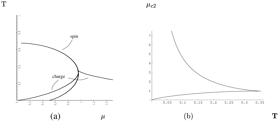
FIG. 1.: (a): Lines of diverging spin glass susceptibility, bending smoothly around from $(T=.6767,\mu=0)$ to $(T=0,\mu=.5)$, and unconventional line $T_{c2}(\mu)$ of divergent replica diagonal nonlinear susceptibility $\chi^{aaaa}$. (b) only the unconventional line is displayed here and given as $\mu_{c2}(T)$.

B Exact low temperature solutions

To analyze solutions of the saddle point equations at low temperatures it is useful to introduce the abbreviation $x=\cosh(\beta\mu)\exp[-1/2\beta^{2}(\tilde{q}-q)]$ and to integrate the difference of eqs. (6) and (7)

$$\tilde{q}-q = \int_{y}^{G}\frac{1+\cosh(\beta\sqrt{q}z)x}{(\cosh(\beta\mu)+x)^{2}}$$ (15)

$$= \frac{T}{\sqrt{2\pi q}}\int_{-\infty}^{\infty}dy\frac{1+x\cosh(y)}{(x+\cosh(y))^{2}}=O(T^{3})$$ (16)

$$= \frac{2T}{\sqrt{2\pi q}}+O(T^{3})\ \ ,$$ (17)

surprisingly enough the result is independent of x.
The leading low temperature contributions to the $\tilde{q}$- equation can be integrated exactly. Its relevant asymptotic behavior, needed for the following discussion, is extracted by

$$\tilde{q} = 1-\frac{xT}{\sqrt{2\pi q}}\int_{-\infty}^{\infty}dy\frac{1}{\cosh(y)+x}$$ (18)

$$= 1-\frac{2xT}{\sqrt{2\pi q}}\left\{\begin{array}[]{c}\frac{\pi}{2}\;\;for\;x\to 0\\ \frac{1}{x}\ln(2x)\;\;for\;x\to\infty\end{array}\right.$$ (21)

The behavior of x in the low T limit is determined by the sign of $|\mu|-\beta/2(\tilde{q}-q)=|\mu|-\frac{1}{\sqrt{2\pi q}}$. For $|\mu|<\frac{1}{\sqrt{2\pi q}}$ x vanishes and we obtain $\tilde{q}=1-\sqrt{\frac{\pi}{8}}T\exp[\beta(|\mu|-\frac{1}{\sqrt{2\pi q}})]$, $q=1-\sqrt{\frac{2}{\pi}}T$. For $\mu=\frac{1}{\sqrt{2\pi}}$ x stays finite when T goes to zero and one still has $q(T=0)=\tilde{q}(T=0)=1$. For still larger values of the chemical potential this value decreases, since now x grows exponentially and eq(18) turns into

$$q=\tilde{q}=1-\frac{2xT}{2\pi q}\frac{1}{x}\ln(x)=1-\frac{2}{\sqrt{2\pi q}}(|\mu|-\frac{1}{\sqrt{2\pi q}}).$$ (22)

The last equation is of fourth order in $\sqrt{q}$ and can have several solutions. In the limit $\mu\to\infty$ however the solution becomes unique and an expansion in inverse powers of the chemical potential seems useful. One finds

$$q=\frac{1}{2\pi}(1/\mu^{2}+1/\mu^{4}+O(1/\mu^{6}))\ .$$ (23)

We now compare the free energy of the paramagnetic solution with that of the ordered one.
Below the $\mu_{c2}$–line there exist three paramagnetic solutions, two minima and one maximum of the free energy. The maximum with the lower free energy ($\tilde{q}=1$) is unstable with respect to spin glass order, hence the physical solution is

$$\tilde{q}_{para}=2e^{-\beta\mu}+O(\beta^{2}e^{-2\beta\mu}).$$ (24)

The corresponding free energy at zero temperature is $f_{dis}=-2\mu$, whereas the free energy of the spin glass solution is

$$f_{ordered} = \frac{1}{4}\beta[-2(\tilde{q}-q)+\tilde{q}^{2}-q^{2}]-\mu$$ (26)

$$-T\int_{z}^{G}[\ln(1+\frac{x}{\cosh(\beta\sqrt{q}z)})+\ln(\cosh(\beta\sqrt{q}z)]$$

$$= \frac{-1+q}{\sqrt{2\pi q}}-\mu-\frac{2\sqrt{q}}{2\pi}\int_{0}^{\infty}dz\,z\exp(-\frac{z^{2}}{2})$$ (28)

$$-\frac{2T^{2}}{\sqrt{2\pi q}}\int^{x}_{0}d\tilde{x}\int_{0}^{\infty}dy\frac{1}{\tilde{x}+\cosh(y)}$$

$$= -2-\mu+\frac{1}{\mu}(1/2+\sqrt{\frac{q}{2\pi}}-2\sqrt{\frac{q}{2\pi}}-1/4)$$ (29)

$$= -2\mu+\frac{1}{\mu}(\frac{1}{4}-\frac{1}{2\pi})$$ (30)

Hence at least for large values of the chemical potential this replica symmetric analysis indicates a paramagnetic ground state. On the other hand we know [20] that for half filling the effect of the fermionic space is to lower the temperature of the continuous spin glass transition by a factor of $0.6767$. Hence a transition from spin glass to paramagnet must take place on the zero temperature axis. In order to locate it we solve Eq.(22) for all values of the chemical potential and compare the free energy of the different solutions. Spin glass order is realized up to a chemical potential $\mu=.900$, at this value we find a first order transition with a jump of the order parameter from $q=.603$ to zero. By means of the relation $[\nu]_{av}=2-\tilde{q}$ (valid in this form only at $T=0$) one finds phase separation for fillings $1.34<\nu<2$.
However, a stability analysis of this replica symmetric solution according to the scheme of de Almeida and Thouless [21, 25] reveals two negative eigenvalues of the Hessian matrix instead of the expected one negative value indicating just the instability towards replica symmetry breaking. As described in [3] for spin glass problems, one has to choose the stable solution with the lowest free energy, hence the system undergoes a first order transition from half filling to the completely filled paramagnetic state at $\mu=\frac{1}{\sqrt{2\pi}}J$. The analysis of RPSB in I indicates that this region of incompressibility becomes smaller with increasing order of symmetry breaking. Therefor one may expect that for infinite order RPSB the fermion filling increases continuously from one with increasing chemical potential until it makes a finite jump at a special value of $\mu$.

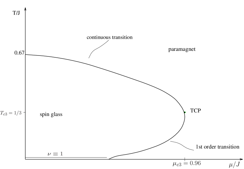
FIG. 2.: Qualitative phase diagram of the $ISG_{f}$ in ($\mu$,T)–space calculated in the replica symmetric approximation

Now we have gathered important information on the global phase diagram of the infinite–range fermionic spin glass model. At $\mu=0$ (half filling) a continuous transition takes place, for increasing $\mu$ the transition temperature is lowered. At zero temperature the transition is first order in both the spin and charge density, therefore it is natural to look for a tricritical point at which the transition changes its character from 2nd order to 1st order. The point $T=J/3,\mu=0.961056$ is a good candidate for tricritical behavior since charge– and spin– fluctuations become simultaneously critical there.

C Tricritical Behavior

Resorting to different techniques we performed a detailed analysis of tricritical behavior in the $ISG_{f}$. Mean field type quantities are most easily calculated from an expansion of the saddle point free energy around the tricritical point given by

$$T_{c3}=J/3\quad{\rm and}\quad\mu_{c3}=\frac{J}{3}arcosh(2\exp(\frac{3}{2}))\simeq.9611J$$ (31)

This expansion reads

$$f - f_{TCP}=\mu-\mu_{c3}-\frac{3h^{2}}{2J}(\delta\tilde{q}-\int_{0}^{1}q(x)dx)$$ (32)

$$+ J\{(\frac{3}{2}r_{g}g-r_{T}\delta T^{2})\delta\tilde{q}+\frac{3}{2}\delta T[(\delta\tilde{q})^{2}$$ (33)

$$- \int^{1}_{0}dxq^{2}(x)]-\frac{3}{2}[\int^{1}_{0}dx[xq^{3}(x)+3q(x)\int^{x}_{0}dyq^{2}(y)]$$ (34)

$$- 3\delta\tilde{q}\int^{1}_{0}dxq^{2}(x)+\frac{1}{4}(\delta\tilde{q})^{3}]-\frac{y_{4}}{4}\int^{1}_{0}dxq^{4}(x)\},$$ (35)

where $\delta\tilde{q}\equiv\tilde{q}-\tilde{q}_{TCP},gJ=\mu-\mu_{c3}+3(\zeta^{-1}J-\mu_{c3})\delta T$ as nonordering field [26], and $\delta T\equiv T-T_{c3}$. The constants are given by $r_{g}=\frac{2\zeta}{3},r_{T}=12(1-\frac{3}{4}\zeta^{-2})$ with $\zeta\equiv tanh(\mu_{c3}/T_{c3})\simeq 0.9938$, and $\mu_{c3}$ as the characteristic chemical potential locating the TCP. The average filling factor corresponding to $\mu_{c3}$ is evaluated as $[\nu_{c3}]_{av}\simeq 1.6625$. Moreover, we derived a fluctuation Lagrangian for the tricritical and finite range $ISG_{f}$; a Lagrangian of the same structure is obtained for generalized models (eg with a transport mechanism) at finite temperature by integrating out dynamical degrees of freedom

$$L = \frac{1}{t}\int d^{d}x{[}-\frac{3}{2}h^{2}\sum Q^{ab}$$ (36)

$$+ \frac{r\kappa_{1}}{(\kappa_{2})^{2}}\sum Q^{aa}+\frac{1}{2}\sum Q^{aa}(-\nabla^{2}+u)Q^{aa}$$ (37)

$$+ \frac{1}{2}Tr^{\prime}(\nabla Q^{ab})^{2}-\frac{1}{t}\sum^{\hskip 17.07182pt\prime}Q^{aa}Q^{bb}-\frac{\kappa_{1}}{3}\sum(Q^{aa})^{3}$$ (38)

$$- \frac{\kappa_{3}}{3}Tr^{\prime}Q^{3}-\kappa_{2}\sum^{\hskip 14.22636pt\prime}Q^{aa}Q^{ab}Q^{ba}+\frac{y_{4}}{4}\sum^{\hskip 14.22636pt\prime}(Q^{ab})^{4}{],}$$ (39)

Here $4(\frac{\kappa_{1}}{t})^{(0)}=(\frac{\kappa_{2}}{t})^{(0)}=(\frac{\kappa_{3}}{t})^{(0)}=\frac{3^{3}}{2}$ and $u^{(0)}=0$ denote the bare coefficients at tricriticality. One fourth order term relevant for replica symmetry breaking is kept. Replicas under $\sum^{\prime}$ or $Tr^{\prime}$ are distinct. The $Q^{aa}Q^{bb}$–coupling is renormalization group generated as in the metallic quantum spin glass, its effects will be discussed in a subsequent section. The simultaneous appearance of critical diagonal and off–diagonal field components is very unusual for classical thermal spin glass transitions and was so far known only to occur in special limits [27].

The tricritical behavior can be extracted from a quadratic approximation of the self - consistency equations. Since replica symmetry breaking is only generated by the $y_{4}$ - term in the free energy in the context of a quadratic approximation it is sufficient to consider the plateau height $q(1)=q_{EA}=q+$ subleading corrections.

$$0 = gr_{g}-r_{T}\delta T^{2}+6\delta T\delta\tilde{q}-\frac{3}{4}\delta\tilde{q}^{2}+3q^{2}$$ (40)

$$0 = 6q(\delta\tilde{q}-\delta T-q)$$ (41)

From (40) we get for q=0

$$\delta\tilde{q}_{dis} = 4(\delta T\pm|\delta T|\sqrt{1+\frac{r_{g}g}{12\delta T^{2}}-\frac{r_{T}}{12}})$$ (42)

$$= 4(\delta T\pm|\delta T|W)$$ (43)

Only the smaller solution (eg that with the - sign) corresponds to a minimum of the free energy; on the line $\delta\mu=-3(1/\zeta-\mu_{c3})\delta T=-0.1354\delta T$ which is tangent to the critical curves $\mu_{c1}(T)$ and $\mu_{c2}(T)$ g vanishes and $\delta\tilde{q}_{dis}$ is proportional to $\delta T$. The statement holds true for a region close to the tangent where $g\sim\delta T^{2}$ as well, there the radicand is positive for $g<-\frac{12-r_{T}}{r_{g}}\delta T^{2}$. This result reproduces an expansion of the exact relation $\mu_{c2}(T)$ around $T=\frac{1}{3}$.

However, if g is of order $\delta T$ or larger the solution becomes to leading order $\delta\tilde{q}=\sqrt{\frac{r_{g}g}{12}}$ and thus displays a nonanalytical dependence on temperature and / or chemical potential. This type of crossover can also be seen in the free energy

$$f_{dis} = \frac{3}{2}|\delta T|^{3}[4(sgn(\delta T)-W)(\frac{r_{g}g}{\delta T^{2}}-r_{T})$$ (45)

$$-48sgn(\delta T)(sgn(\delta T)-W)^{2}-16(sgn(\delta T)-W)^{3}]$$

$$= |\delta T|^{2-\alpha}{\cal G}(\frac{g}{\delta T^{2}})$$ (46)

The scaling form allows for the identification of the specific heat exponent $\alpha=-1$ and the crossover exponent $\phi=2$. The crossover function ${\cal G}(x)$ is regular for small x and has the asymptotic form

$${\cal G}(x){\approx\atop x\to\infty}x^{\frac{2-\alpha}{\phi}}{\cal G}_{\infty}+({\rm regular\hskip 2.84544ptcorrections}).$$ (47)

In the tricritical region the leading singularity in the free energy is given by

$$f_{TCP,sing} = \frac{4}{\sqrt{3}}(r_{g}g)^{\frac{3}{2}}$$ (48)

For $\delta\mu=0$ we have $g\sim\delta T$ and can read off the tricritical specific heat exponent $\alpha_{3}=\frac{1}{2}$ from above.

The next step is the search for ordered solutions of the selfconsistency equations. Using $q=\delta\tilde{q}-\delta T$ one solves readily for

$$\delta\tilde{q}_{ordered}=\pm\frac{2}{3}|\delta T|\sqrt{-\frac{r_{g}g}{\delta T^{2}}+r_{T}-3}$$ (49)

The solution exists for $g<-\frac{\delta T^{2}}{r_{g}}(r_{T}-3)$ (see curve d in figure 2). The corresponding replica overlap q is positive for $q=|\delta T|(-sgn(\delta T)\pm\frac{2}{3}\sqrt{-\frac{r_{g}g}{\delta T^{2}}+r_{T}-3})>0$. For positive $\delta T$ the ”+”- sign needs to be chosen, the condition $q>0$ is then equivalent to $g<-(\frac{21}{4}-r_{T})\frac{\delta T^{2}}{r_{g}}$, which reproduces an expansion of $\mu_{c1}(T)$ (see curve a in figure 2). Considering now the case $\delta T<0$, we get the condition $\pm\frac{2}{3}\sqrt{-\frac{r_{g}g}{\delta T^{2}}+r_{T}-3}>-1$. The ”+” - solution is always o.k., the ”-” - solution only in the region with $-(\frac{21}{4}-r_{T})\frac{\delta T^{2}}{r_{g}}<g<-\frac{\delta T^{2}}{r_{g}}(r_{T}-3)$ (in the region between curve a and d). The saddle point energy for the physically meaningful ”+” - solution is

$$f_{ordered}=-\frac{2}{3}(-\frac{r_{g}g}{\delta T^{2}}-\frac{r_{T}-3}{r_{g}})$$ (50)

The energy difference $f_{ordered}-f_{dis}$ becomes negative for $g<-7.9488\delta T^{2}$ (thermodynamic transition, shown in curve c in figure 2). In the tricritical region the solution of the selfconsistency equations is

$$q=\delta\tilde{q}=\frac{2}{3}\sqrt{-r_{g}g}$$ (51)

which yields the tricritical order parameter exponent $\beta_{3}=\frac{1}{2}$ and suggests that $q$ and $\delta\tilde{q}$ act as order parameters simultaneously. From the fluctuation Lagrangian one reads off mass squared proportional to $\delta T^{2}$ and hence $\gamma_{3}=\beta_{3}=\alpha_{3}=\frac{1}{2}$.

D Replica Symmetry Breaking and tricritical Almeida Thouless - Line

In contrast to crystal–field split spin glasses [23] the quartic coefficient $y_{4}$ of our free energy, Eq.(35), is nonzero and one obtains the Parisi solution

$$q(x)=\left\{\begin{array}[]{l}\frac{9}{2y_{4}}x\quad{\rm for}\quad 0\leq x\leq x_{1}\\ q(1)\quad{\rm for}\quad x_{1}\leq x\leq 1\end{array}\right.$$ (54)

The plateau height is found to satisfy

$$q(1)=\delta\tilde{q}+O(\delta\tilde{q}^{2}).$$ (55)

Consequently, plateau and breakpoint scale like $\sqrt{|\tau|}+O(\tau)$ at the $TCP$, while linear $\tau$-dependence is reserved to $T_{c}>T_{c3}$. Adapting the notation of [29] we express our result for the irreversible response $q(1)-\int^{1}_{0}q(x)\sim|\tau|^{\beta_{\Delta}}$ in terms of the exponent $\beta_{\Delta 3}=1$ for $T\rightarrow T_{c3}$ and $\beta_{\Delta}=2$ for $T\rightarrow T_{c}>T_{c3}$. For the Almeida–Thouless line at tricriticality we find

$$\frac{H^{2}}{J^{2}}=\frac{80}{81}(\frac{2}{3}(1-\frac{\mu_{c3}}{J}tanh(\frac{3\mu_{c3}}{J})))^{3/2}\tau_{AT}^{3/2}+O(\tau_{AT}^{2})$$ (56)

with $\tau_{{AT}}\equiv\frac{T_{c3}-T_{AT}(H)}{T_{c3}}$. Hence we obtain the critical exponent $\theta_{3}=\frac{4}{3}$ near $T_{c3}$, while $\theta=\frac{2}{3}$ for all $T_{c}>T_{c3}$. These values do not satisfy the scaling relation $\theta_{3}=\frac{2}{\beta_{\Delta_{3}}}$ with $\beta_{\Delta_{3}}=1+(\gamma_{3}-\alpha_{3})/2$. Along the lines described in [29], this problem of mean–field exponents will be resolved below by the renormalization group analysis of the coupling $y_{4}$ of the finite–range and finite–dimensional $ISG_{f}$.

E Stability of the solution in the tricritical region

A first test for stability of the saddle point solutions is looking at the (matrix) of second derivatives of the free energy with respect to q and $\delta\tilde{q}$.

$$\frac{\partial^{2}f}{\partial\tilde{q}^{2}} = 9\delta T-\frac{9}{4}\delta\tilde{q}+O(q^{2},\delta\tilde{q}^{2})$$ (57)

$$\frac{\partial^{2}f}{\partial q^{2}} = 9(-\delta T+\delta\tilde{q}-2q)$$ (58)

In the tricritical regime $\delta\tilde{q}$ and $q$ are leading compared to the temperature deviation. The stability condition $\frac{\partial^{2}f}{\partial q^{2}}<0$ is satisfied both in the ordered and in the disordered regime, whereas $\frac{\partial^{2}f}{\partial\tilde{q}^{2}}$ is positive in the paramagnetic phase and negative (e.g. unstable) in the ordered phase. One may wonder whether the coupling between diagonal and offdiagonal fluctuations cures this problem or whether there is a new type of instability in addition to the well known AT - instability. . The $\delta Q^{aa}$ - fluctuations are vectors in replica space and play the role of the $\delta m^{a}$ -fluctuations in the notation of Almeida and Thouless, the matrix entries A, B, C and D of AT are replaced by (to order $\sqrt{g}$)

$$X = \frac{1}{2}\beta^{2}[1-\frac{1}{2}\beta^{2}(<(\sigma^{a})^{4}>-<(\sigma^{a})^{2}>^{2})]$$ (59)

$$= -\frac{27}{4}\delta\tilde{q}$$ (60)

$$Y = -\beta^{4}(<(\sigma^{a})^{2}(\sigma^{b})^{2}>-<(\sigma^{a})^{2}><(\sigma^{b})^{2}>)$$ (61)

$$= 0$$ (62)

$$V = -\beta^{4}(<(\sigma^{a})^{3}\sigma^{b}>-<(\sigma^{a})^{2}><\sigma^{a}\sigma^{b}>)$$ (63)

$$= -54q$$ (64)

$$W = -\beta^{4}(<(\sigma^{a})^{2}\sigma^{b}\sigma^{c}>-<(\sigma^{a})^{2}><\sigma^{b}><\sigma^{c}>)$$ (65)

$$= 0$$ (66)

P, Q and R control as usually offdiagonal fluctuations and are given by

$$P = \beta^{2}[1-\beta^{2}(<(\sigma^{a})^{2}(\sigma^{b})^{2}>-<\sigma^{a}\sigma^{b}>^{2})]$$ (67)

$$= -54\delta\tilde{q}$$ (68)

$$Q = -\beta^{4}(<(\sigma^{a})^{2}\sigma^{b}\sigma^{c}>-<\sigma^{a}\sigma^{b}><\sigma^{a}\sigma^{c}>)$$ (69)

$$= -27q$$ (70)

$$R = -\beta^{4}(<\sigma^{a}\sigma^{b}\sigma^{c}\sigma^{d}>-<\sigma^{a}\sigma^{b}><\sigma^{c}\sigma^{d}>=0$$ (71)

In the limes $n\to 1$ AT obtained five eigenvalues, one of them ($P-2Q+R$) is not related to diagonal fluctuations, the other four merge in the replica limit to

$$\lambda_{\pm} = \frac{1}{2}(X-Y+P-4Q+3R$$ (73)

$$\pm\sqrt{(X-Y-P+4Q-3R)^{2}-8(V-W)^{2}}$$

$$= \frac{1}{2}(X+P-4Q\pm\sqrt{(X-P+4Q)^{2}-8V^{2}}$$ (74)

$$= \frac{27q}{8}(7\pm i\sqrt{2^{9}-3^{4}})$$ (75)

The real part of these eigenvalues is positive and guarantees stability, the logarithm of the partition function stays real in spite of the imaginary part of the eigenvalues, it contains a factor

$$\frac{1}{\sqrt{(\lambda_{+}\lambda_{-})(\lambda_{+}\lambda_{-})^{(}n-1)}}$$ (76)

which is real in the replica limit.

F Tricritical behavior in the Spin 1 Ising model in transverse fields

The quantum phase transitions at $T=0$ of metallic spin glasses and of the transverse field Ising spin $\frac{1}{2}$ glass were recently described in a unifying quantum field theoretical way. The essential difference between the two being the marginal relevance of the quantum dynamical interaction of transverse field models in contrast to their (dangerous) irrelevance in the metallic case. Similar properties of the phase diagrams of spin 1 and of the $ISG_{f}$ suggest a comparison between quantum extensions of these two models. The Spin 1 Ising spin glass in a transverse field will see its thermal tricritical point descend towards zero temperature as the transverse field approaches a characteristic value. Again, as in the metallic case, we approximate this value by a Q–static approximation, improving this result finally by a generalized Miller–Huse method [28].

G Renormalization Group Analysis

1 Tricritical Ising Spin Glass

We performed a 1–loop RG calculation for tricritical fluctuations. At each RG step the mass of charge fluctuations $\delta Q^{aa}$ was shifted away. Introducing the anomalous dimensions $\tilde{\eta}$ and $\eta$ for diagonal and offdiagonal fluctuations one finds at one loop level the following RG relations ($\epsilon=8-d$)

$$\frac{dr}{dl} = (\frac{d}{2}-11\kappa^{2}_{1}+16\kappa_{1}\kappa_{2}+6\kappa^{2}_{2})r-\kappa^{2}_{2}$$ (77)

$$\frac{du}{dl} = 2(1-\kappa_{1}^{2})u-4\kappa_{1}^{2}+4\kappa_{1}\kappa_{2},$$ (78)

$$\frac{d\kappa_{1}}{dl} = \frac{\epsilon}{2}\kappa_{1}+9\kappa_{1}^{3}\,\frac{d\kappa_{2}}{dl}=(\frac{\epsilon}{2}+6\kappa^{2}_{2}-\kappa_{1}^{2}+16\kappa_{1}\kappa_{2})\kappa_{2}$$ (79)

$$\frac{d\kappa_{3}}{dl} = (\frac{\epsilon}{2}+9\kappa^{2}_{2})\kappa_{3},$$ (80)

Above $d=8$ the RG flows towards the Gaussian fixed point with mean field exponents, for $d<8$ there is no perturbatively accessible fixed point for real $\kappa^{\prime}s$. However, a preliminary analysis of the resulting strong coupling problem shows that there exists a solution with positive $\tilde{\eta}$ in contrast to the negative anomalous dimension typical of cubic field theories with imaginary coupling. The RG for the $DIC$ $y_{4}$ showed that its long–distance behavior is dominated by a $\kappa^{4}$–contribution (like in [29] but) for $d_{c}^{(u)}=8<d<10$. This leads to the modified MF exponent $\theta_{3}=8/(d-4)$, which satisfies the scaling relation $\theta_{3}=2/\beta_{\Delta_{3}}$ in $d_{c3}^{(u)}=8$ and reduces to the MF–result in $10$ dimensions. The dimensional shift by $2$ in comparison with [29] is due to coupling $t$.

2 Metallic Quantum Spin Glass

In the theory of quantum phase transitions time–dependent fluctuations are treated on an equal footing with spatial fluctuations [18]. While for the Lagrangian (35) it was sufficient to consider only the $\omega=0$ - component of the Q - fields, in the quantum case all low energy fields must be kept as they are coupled via the quantum mechanical interaction $u\int d\tau(Q^{aa})^{2}$. However, the value $z=4$ of the dynamical critical exponent renders the u - coupling dangerously irrelevant and allows for a perturbative mapping of the critical theory on a classical problem, the Pseudo - Yang - Lee edge singularity. This field theory has only one cubic coupling which corresponds to $\kappa_{1}$ in eq(35). The comparison of the metallic quantum case with the thermal tricritical theory allows one to understand the nature of the strong coupling RG fixed point: whereas the spin fluctuations in the thermal second order regime are governed by a perturbatively accessible fixed point, the TCP and the quantum case are characterized by the combination of charge and spin fluctuations and a corresponding strong coupling problem.

III The paramagnetic phase: Multiple low temperature saddle–point solutions

Complications due to variation of the chemical potential can also be seen outside the spin glass phase of the fermionic Ising spin glass. We have discussed (see also Fig.(1)) the unusual critical line $\mu_{c2}(T)$, which crosses the spin glass regime and, passing through the thermal tricritical point, stretches into the regime up to arbitrarily large $\mu$. It was seen that in the regime of large particle pressure the spin density becomes small and spin glass order is apparently absent. Despite the presence of the $\mu_{c2}(T)$– or, if one wish, $T_{c2}(\mu)$–line, the absence of magnetic phase transitions caused by the totally frustrated magnetic interaction is predicted by the replica symmetric ordered solution eq.(22). The multitude of paramagnetic solutions below the $T_{c2}(\mu)$–line and a possible metastability in finite range models is discussed in this section. We take advantage of the fact that replica permutation symmetry will play no role. We consider however possible that spontaneous vector replica symmetry breaking [31] will be involved. In the paramagnetic regime one finds three solutions for $\tilde{q}$, and hence for the susceptibility $\chi=\beta\tilde{q}$ too, at temperatures below $T_{c2}(\mu)$. This temperature is given by the inversion of Eq.(14) and is also shown in Fig.(5).
At low temperatures these solutions are well approximated by

$$\tilde{q}\hskip 2.84544pt|_{{}_{{}_{T<<T_{c2}}}}=\left\{\begin{array}[]{l}1\\ 2\mu/\beta+O(\beta^{-2}ln\beta)\\ 2e^{-\beta\mu}\end{array}\right.$$ (84)

These saddle–point solutions for $\tilde{q}$ and the corresponding ones for the linear susceptibility are displayed for a few characteristic values of the chemical potential $\mu$, starting from the tricritical value $\mu_{c3}=0.96125J$. The magnetically saturated solution ($\tilde{q}=1$) which would imply a Curie susceptibility $\chi\sim\beta$ is unstable with respect to spin glass order for all temperature. The high temperature solution, which decays exponentially at low temperatures and leads to a vanishing susceptibility in the zero temperature limit is the physical paramagnetic solution in the whole temperature range. It is not clear however whether a replica symmetry broken stable solution with a possibly lower free energy exists due to the presence of exceptionally strong bonds. The linearly decaying solution is a maximum of the free energy at all temperatures. For large values of the chemical potential the physical solution $\tilde{q}=2e^{-\beta\mu}$ has a much larger free energy than the Curie type solution $\tilde{q}=1$. The two free energy minima are separated only by a very small barrier, hence we expect fluctuations to play a major role in finite range models. The instability of the lower minimum with respect to spin glass order makes it conceivable that due to Griffiths effects a replica symmetry broken ordered solution persists in the region of very low T for all values of the chemical potential.

FIG. 3.: Spin autocorrelation function shown for various chemical potentials $\mu=.96125J(a),J(b),2J(c),$ and $10J(d)$ with three low temperature solutions of the paramagnetic saddle-point equation: the lowest one (indistinguishable over a wide range from the $\beta$–axis on the given scale) is the only stable minimum of the free energy.

FIG. 4.: Linear susceptibility corresponding to the three solutions of the paramagnetic saddle–point equation, given for $\mu=1$, $\mu=3$, which are joined in the fourth figure (bottom right); the first one (top left) shows the solution near the tricritical chemical potential for comparison. The (sole) high temperature solution remains realized at all temperatures.

FIG. 5.: Paramagnetic free energy as a function of $\tilde{q}$ for $\mu=3J$ and $\beta=10/J$ (curve a),$\beta=20/J$ (b), and $\beta=50/J$ (c).

IV Relations with the Blume-Emery-Griffiths model for $He^{3}-He^{4}$ mixtures; universal mean field tricritical point

For classical spin systems there exists a variety of different ways to describe diluted systems. Spin 1 models, where $S_{i}=0$ may be considered to describe an empty site i, provide one example. A beautiful case was formulated by Syozi, who extended Onsager’s solution to the twodimensional diluted Ising ferromagnet. Another example is given by the Blume-Emery-Griffith model intended to describe $He^{3}-He^{4}$ mixtures, where the $S_{i}=0$ state corresponds to a $He^{3}$-atom on site i. Disorder effects added to the original BEG model have raised considerable interest recently [30]. But it is in fact the clean BEG model that shows the perhaps accidental but in any case most eyecatching resemblance with part of the fermionic Ising spin glass tricritical behavior. There is a surprisingly identical tricritical temperature $T_{c3}=\frac{1}{3}J$ of the clean BEG without $S^{2}S^{2}$-interaction (ie K=0) on one hand and of the $ISG_{f}$ on the other (the meaning of J being n.n. $J_{ij}$ for the BEG and standard deviation of $J_{ij}$ in case of the spin glass). Another surprising fact is however that it is the $K\neq 0$ BEG-equation for $<S^{2}>$ ($=1-x$ in [22]) which can be mapped onto the $ISG_{f}$-equation for $<(S^{a})^{2}>\sim\tilde{q}$ in the disordered phase. Reconsidering the $\tilde{q}$-equation for $H=m=q=0$ from the selfconsistent $ISG_{f}$-equations given above

$$\tilde{q}=1/[1+cosh(\beta\mu)exp(-\frac{1}{2}\beta^{2}J^{2}\tilde{q})]$$ (85)

and comparing it with the BEG-equation for $m=0$ which reads

$$1-x=1/[1+\frac{1}{2}exp(\beta\Delta)exp(-\beta K(1-x))]$$ (86)

one finds an identical structure in the variables $\tilde{q}$ and $1-x$.

V Phase Separation

Up to now the tricritical phenomenon and the first order transition from paramagnet to spin glass have mainly been discussed for given chemical potential. In this picture a thermodynamical first order transition is observed for $\delta\mu=-0.1355\delta T-7.9488\delta T^{2}$. On this line the free energies of paramagnetic and ordered solution are the same but the two solutions correspond to different fermion fillings of the system. This can be seen from the following consideration: On the first order line we have $\delta\tilde{q}_{dis}=-6.2649|\delta T|$ and $\delta\tilde{q}_{ordered}=1.5133|\delta T|$. Via the relation

$$\delta\nu=-\delta\tilde{q}\tanh(\beta_{c3}\mu_{c3})-\delta T\frac{1}{2e^{3}}$$ (87)

the phase diagram in $(\nu,T)$ space in the neighborhood of the TCP is defined. $\delta\nu_{1}=6.2522|\delta T|$ limits the ordered region, $\delta\nu_{2}=-1.4779|\delta T|$ the disordered region. For intermediate fillings $\delta\nu_{1}<\delta\nu<\delta\nu_{2}$ both phases coexist.

VI The Fermionic Ising Chain

The remarkable similarities between the phase diagrams of the BEG–model without disorder and the one of the fermionic Ising spin glass can be taken as indicative for the fact that rather dilution than disorder is the source of the tricritical crossover from continuous to discontinuous phase transitions. Moreover the RG theory showed that the tricritical structure is also not very sensitive to spatial dimension. These impressions and the fact that mapping of fermionic spin glass transitions to Pseudo Yang Lee edge singularities have been proved may be enough motivation for an analysis of onedimensional cases.
While it is complicated to solve 1D fermionic Ising spin glasses ( no matter whether $d=1$ is below the lower critical dimension or above due to long range interaction) exactly, the clean fermionic Ising chain offers simple exact solutions. These solutions discussed here will provide some insight into the role of the chemical potential and moreover generalize known results into the complex $\mu$–plane.
Yang and Lee [32] derived the distribution of zeroes of the partition function of finite and infinite Ising chains within the complex magnetic field plane. In fermionic Ising systems the chemical potential can be seen as complementary to the magnetic field. Stimulated by the representation of conventional Ising chains by fermionic ones with special imaginary chemical potential, one may wish to extend the Yang Lee analysis to a fourdimensional space $((Re\mu),Im(\mu),Re(h),Im(h))$.
The transfer matrix ${\bf T_{f}}$ of the fermionic Ising chain in a (complex) field $h$ and with (complex) chemical potential $\mu$ reads

$$T_{f} = e^{\beta\mu}\left(\begin{array}[]{*{4}{c}}e^{\beta\mu}&1&e^{\frac{1}{2}\beta(\mu+h)}&e^{\frac{1}{2}\beta(\mu-h)}\\ 1&e^{-\beta\mu}&e^{\frac{1}{2}\beta(h-\mu)}&e^{-\frac{1}{2}\beta(\mu+h)}\\ e^{\frac{1}{2}\beta(\mu+h)}&e^{\frac{1}{2}\beta(h-\mu)}&e^{\beta(J+h)}&e^{-\beta J}\\ e^{\frac{1}{2}\beta(\mu-h)}&e^{-\frac{1}{2}\beta(\mu+h)}&e^{-\beta J}&e^{\beta(J-h)}\end{array}\right)$$ (92)

while the corresponding one of the $S=\pm 1$–chain is given by

$$T_{s}=\left(\begin{array}[]{cc}e^{\beta(J+h)}&e^{-\beta J}\\ e^{-\beta J}&e^{\beta(J-h)}\end{array}\right).$$ (96)

The transfer matrices and their eigenvalues don’t map onto each other at $\mu=i\frac{\pi}{2}T$, but the partition function does according to

$$Z_{f}^{(N)}=TrT_{f}^{N}=(2i)^{N}Z_{s}^{(s)}$$ (97)

for any number N of sites.
The largest eigenvalue determines the free energy of the infinite chain, while the second largest is required in addition to determine the correlation length. The largest eigenvalue results in general from a cubic equation resulting in a lengthy result for the free energy. For several purposes it is sufficient to know the eigenvalues for $(h=0,\mu)$, $\mu$ arbitrary complex. The half–filled case $(\mu=0,h)$, h arbitrary complex, may also be considered separately.
The eigenvalues for $h=0$ are found as

$$\lambda_{\pm} = e^{\beta\mu}[ch(\beta\mu)+ch(\beta J)$$ (99)

$$\pm\sqrt{(ch(\beta\mu)+ch(\beta J))^{2}+4ch(\beta\mu)(1-ch(\beta J))}]$$

$$\lambda_{0} = 0\quad,\quad\lambda_{1}=2e^{\beta\mu}sh(\beta J).$$ (100)

The correlation length is given by

$$\xi=1/ln(\frac{\lambda_{+}}{\lambda_{1}}).$$ (101)

In the $T\rightarrow 0$–limit a transition (formally) arises at $\mu=J$ and due to the properties

$$\lambda_{1} \sim exp(\beta(\mu+J))$$ (102)

$$\lambda_{+} \sim \left\{\begin{array}[]{cc}exp(\beta(\mu+J)),\quad\mu<J\\ exp(2\beta\mu),\quad\mu>J\end{array}\right.$$ (105)

Thus the correlation length diverges only for $\mu<J$, which is comprehensible since the energy required for adding a fermion is larger than the gain from a magnetic bond if $\mu>J$. One obtains

$$\xi\sim\left\{\begin{array}[]{c}exp(\beta(2J-\mu))\quad,0<\mu<J\\ \exp(\beta J/2\quad,\mu=J.\end{array}\right.$$ (108)

while $\xi\sim T/(\mu-J)$ for $\mu>J$. Taking the derivative of the free energy $f=-Tln\lambda_{+}$ w.r.t. the chemical potential yields the filling factor showing that in the zero temperature limit the system is completely filled provided $\mu$ is positive (empty for negative $\mu$). Thus there is no physical $T=0$–transition of this simple system. The correlation length diverges in the $T\rightarrow 0$ limit for all fillings $\nu$.
The zero–field partition function shows that Yang–Lee zeroes approach $|\mu|=\pm J$ for $T\rightarrow 0$. This means that for $(h=0,T=0)$ nonanalytic behavior (as a function of the real chemical potential) can only occur at the values $\mu=\pm J$.
It is instructive to consider $N=2$ explicitly, which yields

$$Z^{N=2}_{f} = 4e^{2\beta\mu}[(ch(\beta\mu)+ch(\beta J))^{2}$$ (110)

$$+ch^{2}(\beta h)(e^{2\beta J}-1)-sh(2\beta J)]$$

This almost trivial case already shows zeroes at

$$\mu_{0}=\pm(J+(\frac{1}{2}ln2\pm i\frac{\pi}{2})T)$$ (111)

while allowing for finite complex magnetic field the first zero different from $\pm J$ in the $T\rightarrow 0$–limit becomes possible with

$$\mu=\pm(i\frac{\pi}{4}+2im\pi)T=\mu+im\pi T.$$ (112)

More zeroes occur on the $T=0$–axis as N is increased. In the $N\rightarrow 0$–limit a density function is expected in accordance with the divergent behavior of the correlation length for any $\mu$. Its evaluation is beyond the scope of this paper.

VII Mapping the twodimensional Ising model with imaginary magnetic field $h=\frac{i\pi}{2}T$ into fermionic space

The complementary role of complex magnetic field and complex chemical potential can nicely be seen by recalling that the 2d Ising model with nonreal magnetic field had only been solved exactly at the special value $H=i\frac{1}{2}\pi T$. This value corresponds to $\mu=i\frac{1}{2}\pi T$, which maps the fermionic Ising model onto the one above. Thus the exact solution of the 2d fermionic Ising model with $\mu=H=i\frac{1}{2}\pi T$ is known. Moreover this special model maps onto an interacting model which describes the interaction of spinless fermions with a special species obeying bare Bose statistics but carrying along the minus signs of fermion interactions. The Hamiltonian of this model can be written

$$H=-\sum_{ij}J_{ij}\sigma_{i}^{z}\sigma_{j}^{z}-\mu\sum_{i}(n_{i\uparrow}+n_{i\downarrow})-h\sum_{i}\sigma_{i}^{z}$$ (113)

with $\mu=h=i\frac{\pi}{2}T$. While this value of $\mu$ provides the desired map between 2–state– and 4–state–per–site–space for any magnetic field, the special value considered here reduces to zero the imaginary field of one fermionic species, while the other acquires a shift equal to the distance between Bose– and Fermi–Matsubara energies.
Setting $c=a_{\uparrow}$ and $d=a_{\downarrow}$ the Hamiltonian reads

$$H = -\sum_{ij}J_{ij}[c^{\dagger}_{i}c_{i}c^{\dagger}_{j}c_{j}-c^{\dagger}_{i}c_{i}d^{\dagger}_{j}d_{j}-d_{i}^{\dagger}d_{i}c_{j}^{\dagger}c_{j}+d^{\dagger}_{i}d_{i}d^{\dagger}_{j}d_{j}]-$$ (115)

$$i\pi T\sum_{i}d^{\dagger}_{i}d_{i}.$$

The effect of the new imaginary chemical potential $i\pi T$ acting only on the d–fermions can both be imagined in standard many body diagram theory and within the fermionic path integral representation. In both formalisms the fermionic Matsubara energies of the d–fermions become bosonic ones. In other words d–propagators become bosonic while c–propagators remain (unchanged) fermionic. All interactions (vertices) between c–fermions and d–particles remain fermionic in character, ie they carry the minus–signs due to the anticommutation rules of the operators c and d. In the fermionic path integral representation Grassmann–fields are indispensable for both c– and d–operators. Denoting them by $\psi_{c}(\tau)$ and by $\psi_{d}(\tau)$ respectively, the important change due to the $i\pi T\hat{n}_{d}$–term, which we absorb by the phase transformation $exp(i\pi\tau)\psi(\tau)=\tilde{\psi}(\tau)$ in the new anticommuting fields $\tilde{\psi}$, occurs in the unusual periodicity of $\psi_{d}(\tau)$ on the imaginary time axis:

$$\tilde{\psi}_{d}(\tau)=\tilde{\psi}_{d}(\tau+\beta)$$ (116)

while $\psi_{c}(\tau)=-\psi_{c}(\tau+\beta)$ retain the fermionic antiperiodicity. The periodic behavior of the $\psi_{d}$’s purports of course into the bosonic propagator form.
So far the mapping has been exact. In a perturbatively exact way one can even go beyond the above conclusion by stating that the 2D Ising model for this special imaginary magnetic field maps onto a coupled Fermi–Bose system (c–d) with the speciality that any d–loop contributes additional $(-1)$–factors. Despite the speciality of identical coupling constants $J_{ij}$ between all species this system is physical in the sense that there are no imaginary fields, but the mapping of the known solution of the 2d Ising model discussed above is of order by order character.

VIII Acknowledgement

Research presented in this paper (II) and in the preceding paper (I) was supported by the Deutsche Forschungsgemeinschaft under project Op28/5–1, by the SFB410 of the DFG, and by the Deutsche Studienstiftung.
We benefitted from hints by C. De Dominicis, B. Derrida, J. Hertz, D. Sherrington, from continued support by H.A. Weidenmüller, and from critical comments of our coworkers at Würzburg H. Feldmann and M. Rehker.

REFERENCES

- [1] Parisi, G., J. Phys., A13 1101 (1980)
- [2] Parisi, G., J. Phys., A13 L115 (1980)
- [3] K. Binder, and A. P. Young, Rev. Mod. Phys., 58, 801 (1986)
- [4] Fischer, K.H., Hertz, J., Spin glasses, Cambridge Univ. Press 1991
- [5] R. Rammal, G. Toulouse, and M. A. Virasoro, Rev. Mod. Phys. 58, 765 (1986)
- [6] B. Rosenow and R. Oppermann, Phys. Rev. Lett. 77, 1608 (1996)
- [7] L. Onsager, Phys. Rev. 65, 117 (1944)
- [8] C. Itzykson , Nucl. Phys. B 210 (FS6), 448 (1982)
- [9] J.–B. Zuber and C. Itzykson, Phys. Rev. D 15, 2875 (1977)
- [10] J. A. Mydosh, J. Magn. Magn. Mat. 157/158, 606 (1996)
- [11] Süllow, S., Nieuwenhuys, G.J., Menovsky, A., Mydosh, J.A., Mentink, S., Mason, A., Buyers, W., Phys. Rev. Lett.78, 354 (1997)
- [12] F. Steglich, TU–Darmstadt–preprint (1997)
- [13] Peihua Dai, Youzhu Zhang, and M.P. Sarachik, Phys. Rev. Lett. 69, 1804 (1992)
- [14] A. Sengupta and A. Georges, Phys. Rev. B 52 10295 (1995).
- [15] Y. Goldschmidt, Pik–Yin Lai, Phys. Rev. Lett. 64, 2467 (1990)
- [16] G. Buettner, K. D. Usadel, Phys. Rev. B 42 , 6385 (1990)
- [17] D. Thirumalai, Q. Li, and T.R. Kirckpatrick, J. Phys. A 22, 3339 (1989)
- [18] S. Sachdev, N. Read, and R. Oppermann, Phys. Rev. B 52 10286 (1995).
- [19] N. Read, S. Sachdev, J. Ye, Phys. Rev. B52 384 (1995).
- [20] R. Oppermann, A. Mueller - Groeling, Nucl. Phys B 401, 507 (1993)
- [21] J. R. L. de Almeida, D. J. Thouless, J. Phys. A 11, 983 (1978)
- [22] M. Blume, V. J. Emery, and R. B. Griffiths, Phys. Rev. A4, 1071 (1971).
- [23] P. J. Mottishaw, D. Sherrington, J. Phys. C 18, 5201 (1985).
- [24] A. Theumann and M. Vieira Gusmao, Phys. Lett. 105 A, 311 (1984), see also A. Theumann, Phys. Rev. B 56, 5500 (1997)
- [25] F.A. da Costa, C.S.O. Yokoi, and S.R.A. Salinas, J. Phys. A 27, 3365 (1994)
- [26] I. D. Lawrie and S. Sarbach, in Phase Transitions and Critical Phenomena edited by C. Domb and J. L. Lebowitz (Academic Press, London, 1984), p.1
- [27] J. E. Green, A. J. Bray, M. A. Moore, J. Phys. A 15, 2307 (1982).
- [28] D. Huse and J. Miller, Phys. Rev. Lett. 70, 3147 (1993).
- [29] D. S. Fisher and H. Sompolinsky, Phys.Rev.Lett.54, 1063 (1985).
- [30] A. Falicov and A.N. Berker, Phys. Rev. Lett. 76, 4380 (1996)
- [31] V. Dotsenko and M. Mézard, cond–mat/961101
- [32] T. D. Lee, C. N. Yang, Phys. Rev. 87, 410 (1952)