Intensity distribution for waves in disordered media: deviations from Rayleigh statistics

Abstract

We study the intensity distribution function, $P(I)$, for monochromatic waves propagating in quasi one-dimensional disordered medium, assuming that a point source and a point detector are embedded in the bulk of the medium. We find deviations from the Rayleigh statistics at moderately large $I$ and a logarithmically-normal asymptotic behavior of $P(I)$. When the radiation source and the detector are located close to the opposite edges of the sample (on a distance much less then the sample length), an intermediate regime with a stretched-exponential behavior of $P(I)$ emerges.

1. When a wave propagates through a random medium, it undergoes multiple scattering from inhomogeneities. The scattered intensity pattern (speckle pattern) is highly irregular and should be described in statistical terms. One of its characteristics is the intensity distribution, $P(I)$, at some point ${\bf{r}}$. Almost a century ago Lord Rayleigh, using simple statistical arguments, proposed a distribution which bears his name:

$$P_{o}(\tilde{I})=\exp(-\tilde{I})\ ,$$ (1)

where $\tilde{I}$ is the intensity normalized to its average value, $\tilde{I}=I/\langle{I}\rangle$. The Rayleigh distribution has moments $\langle{\tilde{I}^{n}}\rangle=n!$ and it provides, in many cases, a rather accurate fit to experimental data, as long as $I$ is not too large [1]. For large $I$, however, the data show large deviations from Eq. (1) [1, 2, 3]. Various extensions of Eq. (1) have been proposed in the literature. Jakeman and Pusey [4] proposed to fit the data with the K-distribution. It contains a phenomenological parameter $\eta$ and its moments are given by $\langle{\tilde{I}^{n}}\rangle=n!\eta^{-n}\Gamma(n+\eta)/\Gamma(\eta)$. The experimentally relevant situation corresponds to $\eta\gg 1$. In this case moments up to $n\lesssim\eta$ can be approximated as

$$\langle{\tilde{I}^{n}}\rangle\simeq n!\exp(n^{2}/\eta)\ ,$$ (2)

where only the leading term in the exponent has been kept. Thus, only low moments $(n\ll\sqrt{\eta})$ are close to the Rayleigh value $n!$. Some theoretical support to the phenomenological formula Eq. (2) has been given by Dashen [5] who considered smooth disorder (typical size of inhomogeneities much larger than the wavelength).

More recently, there was a considerable theoretical activity in studying the statistics of the transmission coefficients $t_{ab}$ of a one-dimensional sample with short-range disorder [6, 7, 8, 9]. In this formulation of the problem, a source and a detector of the radiation are located outside the sample. The source produces a plane wave injected in an incoming channel $a$, and the intensity in an outgoing channel $b$ is measured. It was shown in [7, 8, 9] that the distribution of the normalized transmission coefficients $s_{ab}=t_{ab}/\langle t_{ab}\rangle$ crosses over from the Rayleigh distribution $P(s_{ab})=e^{-s_{ab}}$ to a stretched-exponential one $P(s_{ab})\sim e^{-2\sqrt{gs_{ab}}}$, where $g$ is the dimensionless conductance.

In this paper we consider a different situation, when both the source and the detector of the radiation are embedded into the bulk of the sample, and calculate the intensity distribution $P(I)$ in this case. We prove that, for not too large $n$, the moments can be indeed described by Eq.(2), and compute the parameter $\eta$ phenomenologically introduced in [4]. We compute further the whole distribution function $P(I)$ and show that its asymptotic behavior at large $I$ is of a logarithmically-normal form, in contrast to the stretched-exponential asymptotics of $P(t_{ab})$ found in Refs.[7, 8, 9]. Finally, we discuss how these two different forms of the asymptotic behavior match each other and describe physical mechanisms governing both of them.

2. We assume a quasi one-dimensional geometry, i.e. consider a tube of transverse dimension $W$ and length $L\gg W$, filled with scattering medium (Fig. 1). The monochromatic source of radiation is placed at point ${\bf{r_{o}}}$. The field at some point ${\bf{r}}$ is given by the (retarded) Green’s function $G_{R}({\bf{r}},{\bf{r_{o}}})$ and the radiation intensity is defined as $I({\bf{r}},{\bf{r_{o}}})\equiv|G_{R}({\bf{r}},{\bf{r_{o}}})|^{2}$. The average intensity $\langle{I({\bf{r}},{\bf{r_{o}}})}\rangle$ is represented diagrammatically in Fig 2. It consists of a diffusion ladder (a diffuson), $T({\bf{r_{1}}},{\bf{r_{2}}})$, attached to two external vertices. The vertices are short-range objects and can be approximated by a $\delta$-function times $(\ell/4\pi)$, so that $\langle{I({\bf{r}},{\bf{r_{o}}})}\rangle=(\ell/4\pi)^{2}T({\bf{r}},{\bf{r_{o}}})$. For the quasi one-dimensional geometry, the expression for the diffuson reads

$$T({\bf r},{\bf r_{o}})=\left(\frac{4\pi}{\ell}\right)^{2}\frac{3}{4\pi}\frac{\left[z_{<}(L-z_{>})\right]}{A\ell L}$$ (3)

where $\ell$ is the elastic mean free path, $A$ is the cross-section of the tube, $z$-axis is directed along the sample, $z_{<}=\text{min}(z,z_{o})$ and $z_{>}=\text{max}(z,z_{o})$. We assume, of course, that $|z-z_{0}|\gg W$.

The intensity distribution $P(I)$, in the diagrammatic approach, is obtained by calculating the moments $\langle{I^{n}}\rangle$ of the intensity. In the leading approximation [10], one should draw $n$ retarded and $n$ advanced Green’s functions and insert ladders between pairs $\left\{G_{R},G_{A}\right\}$ in all possible ways. This leads to $\langle{I^{n}}\rangle=n!\langle{I}\rangle^{n}$ and, thus, to Eq. (1).

Corrections to the Rayleigh result come from diagrams with intersecting ladders, which describe interaction between diffusons. The leading correction is due to pairwise interactions. The diagram in Fig. 3 represents a pair of ”colliding” diffusons. The algebraic expression for this diagram is

$$C({\bf{r}},{\bf{r_{o}}}) = 2\left(\frac{\ell}{4\pi}\right)^{4}\int\left(\prod_{\imath=1}^{4}d^{3}{\bf{r_{\imath}}}\right)$$ (4)

$$\times T({\bf{r}},{\bf{r_{1}}})T({\bf{r}},{\bf{r_{2}}})T({\bf{r_{3}}},{\bf{r_{o}}})T({\bf{r_{4}}},{\bf{r_{o}}})$$ (5)

$$\times \left\{\left(\frac{\ell^{5}}{48\pi k^{2}_{o}}\right)\int d^{3}{\mathchoice{{\hbox{\boldmath$\displaystyle\rho$}}}{{\hbox{\boldmath$\textstyle\rho$}}}{{\hbox{\boldmath$\scriptstyle\rho$}}}{{\hbox{\boldmath$\scriptscriptstyle\rho$}}}}\left[(\nabla_{1}+\nabla_{2})\cdot(\nabla_{3}+\nabla_{4})\right.\right.$$ (6)

$$+ 2\left.\left.(\nabla_{1}\cdot\nabla_{2})+2(\nabla_{3}\cdot\nabla_{4})\right]\prod_{\imath=1}^{4}\delta({\mathchoice{{\hbox{\boldmath$\displaystyle\rho$}}}{{\hbox{\boldmath$\textstyle\rho$}}}{{\hbox{\boldmath$\scriptstyle\rho$}}}{{\hbox{\boldmath$\scriptscriptstyle\rho$}}}}-{\bf{r_{\imath}}})\right\}\ ,$$ (7)

where $k_{o}$ is the wave number and $\nabla_{\imath}$ acts on ${\bf{r_{\imath}}}$. The factor $\left(\ell/4\pi\right)^{4}$ comes from the 4 external vertices of the diagram, the $T$’s represent the two incoming and two outgoing diffusons and the expression in the curly brackets corresponds to the internal (interaction) vertex [11]. Finally, the factor 2 accounts for the two possibilities of inserting a pair of ladders between the outgoing Green’s functions. Integrating by parts and employing the quasi one-dimensional geometry of the problem, we obtain (for $z_{o}<z$):

$$C(z,z_{o})\simeq 2\langle{I(z,z_{o})}\rangle^{2}\left(1+\frac{4}{3\gamma}\right)\ ,$$ (8)

where $\langle{I(z,z_{o})}\rangle={3\over 4\pi}{z_{0}(L-z)\over A\ell L}$ is the average intensity,

$$\gamma=2g{L^{3}\over L^{2}(3z+z_{o})-2Lz(z+z_{o})+2z^{2}_{o}(z-z_{o})}\gg 1\ ,$$ (9)

and $g=k^{2}_{o}\ell A/3\pi L\gg 1$ is the dimensionless conductance of the tube. For simplicity, we will assume that the source and the detector are located relatively close to each other, so that $|z-z_{o}|\ll L$, in which case Eq.(9) reduces to $\gamma=gL^{2}/2z(L-z)$. (All the results are found to be qualitatively the same in the generic situation $z_{0}\sim z-z_{0}\sim L-z\sim L$.)

In order to calculate $\langle{I^{n}}\rangle$ one has to compute a combinatorial factor which counts the number $N_{i}$ of diagrams with $i$ pairs of interacting diffusons. This number is [6] $N_{i}=(n!)^{2}/[{2^{2i}}{i!}{(n-2i)!}]\simeq(n!/i!)(n/2)^{2i}$, so that

$$\frac{\langle{I^{n}}\rangle}{\langle{I}\rangle^{n}}=n!\sum_{\imath=0}^{[n/2]}\frac{1}{i!}\left(\frac{2n^{2}}{3\gamma}\right)^{i}\simeq n!\exp(2n^{2}/3\gamma)\ .$$ (10)

Although $i$ cannot exceed $n/2$, the sum in Eq. (10) can be extended to $\infty$, if the value of $n$ is restricted by the condition $n\ll\gamma$. Eq. (10) represents the leading exponential correction to the Rayleigh distribution. Let us discuss now the effect of higher order “interactions” of diffusons. Diagrams with 3 intersecting diffusons will contribute a correction of $n^{3}/\gamma^{2}$ in the exponent of Eq. (10), which is small compared to the leading correction in the whole region $n\ll\gamma$, but becomes larger than unity for $n\gtrsim\gamma^{2/3}$. Likewise, diagrams with 4 intersecting diffusons produce a $n^{4}/\gamma^{3}$ correction, etc. Restoring the distribution $P(I)$, we find

$$P(\tilde{I})\simeq\exp\left(-\tilde{I}+\frac{2}{3\gamma}\tilde{I}^{2}+O\left({\tilde{I}^{3}\over\gamma^{2}}\right)+\ldots\right)\ ,$$ (11)

It should be realized that Eq. (11) is applicable only for $\tilde{I}\ll\gamma\sim g$ and, thus, does not determine the far asymptotics of $P(I)$. The latter is unaccessible by the perturbative diagram technique and is handled below by the supersymmetry method.

3. In the supersymmetry formalism, averaging over disorder is replaced by functional integration over supermatrix fields, $Q({\bf{r}})$, which satisfy the constraint $Q^{2}=1$ [12]. For technical simplicity, we will assume that the time reversal symmetry is broken by some magnetooptical effects. The integration is done with a weight function $\exp[-S\{Q\}]$, where $S\{Q\}$ is the $\sigma$-model action,

$$S\{Q\}=-\frac{\pi\nu D}{4}\int d^{3}{\bf{r}}\,{\rm Str}(\nabla Q)^{2}\ ,$$ (12)

Str denotes the supertrace, $D$ is the diffusion constant, and $\nu$ is the average density of states. In the considered quasi-1D geometry, $\pi\nu D=gL/2A$, and the field $Q$ depends on the $z$-coordinate only, yielding $S\{Q\}=-(gL/8)\int dz\,{\rm Str}(dQ/dz)^{2}$. Following the derivation outlined in [13, 14, 15], the moments of the intensity at point ${\bf{r}}$ due to the source at ${\bf{r_{o}}}$ are given by

$$\langle{I^{n}}\rangle=\left(-\frac{k_{0}^{2}}{16\pi^{2}}\right)^{n}\int[{\cal D}Q]\left(Q^{bb}_{12}(z)\right)^{n}\left(Q^{bb}_{21}(z_{0})\right)^{n}e^{-S\{Q\}},$$ (13)

where $Q^{bb}_{12}(Q^{bb}_{21})$ is the retarded-advanced (resp. advanced-retarded) matrix element in the boson-boson sector of $Q$. Assuming again that the two points ${\bf{r}}$ and ${\bf{r_{o}}}$ are sufficiently close to each other, $|z-z_{0}|\ll L$ and taking into account slow variation of the $Q$-field along the sample, we can replace the product $Q^{bb}_{12}(z)Q^{bb}_{21}(z_{0})$ by $Q^{bb}_{12}(z)Q^{bb}_{21}(z)$. We get then the following result for the distribution of the dimensionless intensity $y=(16\pi^{2}/k_{0}^{2})I$:

$$P(y)=\int dQ\delta(y+Q^{bb}_{12}Q^{bb}_{21})Y(Q)\ ,$$ (14)

where $Y(Q)$ is a function of a single supermatrix $Q$ defined as follows [13, 15]:

$$Y(Q_{o})\equiv\int_{Q({\bf{r_{o}}})=Q_{o}}[{\cal D}Q]\exp[-S\{Q\}]\ .$$ (15)

In general, the function $Y(Q)$ depends only on the parameters $1\leq\lambda_{1}<\infty$, $-1\leq\lambda_{2}\leq 1$ entering the standard parametrization of the $Q$-matrices [16]. Performing the integration over the other degrees of freedom, we find

$$P(y) = \left(\frac{d}{dy}+y\frac{d^{2}}{dy^{2}}\right)\int d\lambda_{1}d\lambda_{2}$$ (16)

$$\times \left(\frac{\lambda_{1}+\lambda_{2}}{\lambda_{1}-\lambda_{2}}\right)Y(\lambda_{1},\lambda_{2})\delta(y+1-\lambda^{2}_{1})\ .$$ (17)

The evaluation of $Y(Q_{o})=Y(\lambda^{o}_{1},\lambda^{o}_{2})$ involves, by its definition (15), an integration over all supermatrix fields, which assume a given value $Q_{o}$ at point $z_{0}$ and satisfy the boundary conditions $Q|_{z=0,L}=\Lambda$, where $\Lambda\equiv{\rm diag}\{1,1,-1,-1\}$. Since $g\gg 1$, this calculation can be done by the saddle point method, as suggested by Muzykantskii and Khmelnitskii [17]. The result is [15]

$$Y(\lambda_{1},\lambda_{2})\simeq\exp\left\{-\frac{\gamma}{2}\left[\theta^{2}_{1}+\theta^{2}_{2}\right]\right\}\ .$$ (18)

where $\lambda_{1}\equiv\cosh\theta_{1}$, $\lambda_{2}\equiv\cos\theta_{2}$ ($0\leq\theta_{1}<\infty$, $0\leq\theta_{2}\leq\pi$). In fact, the dependence of $Y$ on $\theta_{2}$ is not important, within the exponential accuracy, because it simply gives a prefactor after the integration in Eq. (17). Therefore, up to a pre-exponential factor, the distribution function $P(y)$ is given by

$$P(y)\sim Y(\lambda_{1}=\sqrt{1+y},\lambda_{2}=1)\sim\exp\left(-\gamma\theta^{2}_{1}/2\right)\ ,$$ (19)

where $\theta_{1}=\ln(\sqrt{1+y}+\sqrt{y})$. Finally, after normalizing $y$ to its average value $\langle{y}\rangle=2/\gamma$, we obtain:

$$P(\tilde{I})\simeq\exp\left\{-\frac{\gamma}{2}\left[\ln^{2}\left(\sqrt{1+2\tilde{I}/\gamma}+\sqrt{2\tilde{I}/\gamma}\right)\right]\right\}\ .$$ (20)

For $\tilde{I}\ll\gamma$, Eq.(20) reproduces the perturbative expansion (11), while for $\tilde{I}\gg\gamma$ it implies the log-normal asymptotic behavior of the distribution $P(\tilde{I})$:

$$\ln P(\tilde{I})\simeq-(\gamma/8)\ln^{2}(8\tilde{I}/\gamma)\ .$$ (21)

4. The log-normal “tail” (21) should be contrasted with the stretched-exponential asymptotic behavior of the distribution of transmission coefficients [7, 8, 9]. Let us briefly discuss, how these two results match each other. Analyzing the expression for the moments (13), we find that when the points $z$ and $z_{0}$ approach the sample edges, $z_{0}=L-z\ll L$, an intermediate regime of stretched-exponential behavior emerges:

$$\ln P(\tilde{I})\simeq\left\{\begin{array}[]{ll}-\tilde{I}+{1\over 3g}\tilde{I}^{2}+\ldots\ ,&\ \ \tilde{I}\ll g\\ -2\sqrt{g\tilde{I}}\ ,&\ \ g\ll\tilde{I}\ll g\left({L\over z_{0}}\right)^{2}\\ -{gL\over 8z_{0}}\ln^{2}\left[16\left({z_{0}\over L}\right)^{2}{\tilde{I}\over g}\right]\ ,&\ \ \tilde{I}\gg g\left({L\over z_{0}}\right)^{2}\ .\end{array}\right.$$ (22)

Thus, when the source and the detector move toward the sample edges, the region of validity of the stretched-exponential behavior becomes broader, while the log-normal “tail” gets pushed further away. In contrast, when the source and the detector are located deep in the bulk, $z_{0}\sim L-z\sim L$, the stretched-exponential regime disappears, and the Rayleigh distribution crosses over directly to the log-normal one at $\tilde{I}\sim g$.

Let us now describe the physical mechanisms standing behind these different forms of $P(\tilde{I})$. The Green’s function $G^{R}({\bf r_{0}},{\bf r})$ can be expanded in eigenfunctions of a non-Hermitean (due to open boundaries) “Hamiltonian” as $G^{R}({\bf r_{0}},{\bf r})=\sum_{i}\psi_{i}^{*}({\bf r_{0}})\psi_{i}({\bf r})(k_{0}^{2}-E_{i}+i\gamma_{i})^{-1}$. Since the level widths $\gamma_{i}$ are typically of order of the Thouless energy $E_{c}\sim D/L^{2}$, there is typically $\sim g$ levels contributing appreciably to the sum. In view of the random phases of the wave functions, this leads to a Gaussian distribution of $G^{R}({\bf r_{0}},{\bf r})$ with zero mean, and thus to the Rayleigh distribution of $I({\bf r_{0}},{\bf r})=|G^{R}({\bf r_{0}},{\bf r})|^{2}$, with the moments $\langle\tilde{I}^{n}\rangle=n!$. The stretched-exponential behavior results from the disorder realizations, where one of the states $\psi_{i}$ has large amplitudes in the both points ${\bf r_{0}}$ and ${\bf r}$. Considering both $\psi_{i}({\bf r_{0}})$ and $\psi_{i}({\bf r})$ as independent random variables with Gaussian distribution and taking into account that only one (out of $g$) term contributes in this case to the sum for $G^{R}$, we find $\langle\tilde{I}^{n}\rangle\sim n!n!/g^{n}$, corresponding to the above stretched-exponential form of $P(\tilde{I})$. Finally, the log-normal asymptotic behavior corresponds to those disorder realizations, where $G^{R}$ is dominated by an anomalously localized state, which has an atypically small width $\gamma_{i}$ (the same mechanism determines the log-normal asymptotics of the distribution of local density of states, see Refs. [15, 18]).

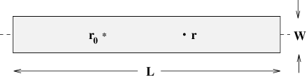
FIG. 1.: Geometry of the problem. Points ${\bf{r_{o}}}=(x_{o},y_{o},z_{o})$ and ${\bf{r}}=(x,y,z)$ are the positions of the source and of the observation point respectively.

FIG. 2.: Diagram for the average intensity. The diffusion ladder is inserted between two solid lines which represent the average Green’s functions.

FIG. 3.: Diagram for a pair of interacting diffusons. The external vertices contribute the factor $(\ell/4\pi)^{4}$. The shaded region denotes the internal interaction vertex, see Eq. 7

- [1] A. Ishimaru, Wave Propagation and Scattering in Random Media (Academic, New York, 1978); J.W. Goodman, J. Opt. Soc. Am. 66, 1145 (1976).
- [2] J.C. Dainty in Laser Speckle and Related Phenomena, edited by J.C. Dainty (Springer-Verlag, Berlin, 1984).
- [3] N. Garcia and A.Z. Genack, Optics Lett. 16, 1132 (1991); A.Z. Genack and N. Garcia, Europhys. Lett. 21, 753 (1993); M. Stoychev and A.Z. Genack, Phys. Rev. Lett. 79, 309, (1997).
- [4] E. Jakeman and P. Pusey, Phys. Rev. Lett. 40, 546 (1978).
- [5] R. Dashen, Optics Lett. 10, 110 (1984).
- [6] E. Kogan, M. Kaveh, R. Baumgartner and R. Berkovits, Phys. Rev. B 48, 9404 (1993).
- [7] Th.M. Nieuwenhuizen and M.C.W. van Rossum, Phys. Rev. Lett. 74, 2674 (1995).
- [8] E. Kogan and M. Kaveh, Phys. Rev. B 52, R3813 (1995).
- [9] S.A. van Langen, P.W. Brouwer and C.W.J. Beenakker, Phys. Rev. E 53, R1344 (1996).
- [10] B. Shapiro, Phys. Rev. Lett. 57, 2168 (1986).
- [11] S. Hikami, Phys. Rev. B 24, 2671 (1981); L.P. Gorkov, A.I. Larkin and D.E. Khmel’nitskii, Sov. Phys. JETP 52, 568 (1980).
- [12] K. Efetov, Supersymmetry in Disorder and Chaos (Cambridge University Press, Cambridge, 1997); K.B. Efetov, Adv. Phys. 32, 53 (1983).
- [13] A.D. Mirlin and Y.V. Fyodorov, J. Phys. A: Math. Gen. 26, L551 (1993); Phys. Rev. Lett. 72, 576 (1994); J. Phys. I France 4, 655 (1994).
- [14] K.B. Efetov and V.N. Prigodin, Phys. Rev. Lett. 70, 1315 (1993); V.N. Prigodin, K.B. Efetov and S. Iida, Phys. Rev. Lett. 71, 1230 (1993).
- [15] A.D. Mirlin, Phys. Rev. B 53, 1186 (1996).
- [16] M. Zirnbauer, Phys. Rev. B 34, 6394 (1984); Nucl. Phys. B 265 (1986).
- [17] B.A. Muzykantskii and D.E. Khmelnitskii, Phys. Rev. B 51, 5480 (1995).
- [18] A.D. Mirlin, J. Math. Phys. 38, 1888 (1997).