Formation of binary correlations in strongly coupled plasmas

Abstract

Employing quantum kinetic equations we study the formation of binary correlations in plasma at short time scales. It is shown that this formation is much faster than dissipation due to collisions, in hot (dense) plasma the correlations form on the timescale of inverse plasma frequency (Fermi energy). This hierarchy of characteristic times is used to derive analytical formulae for time dependency of the potential energy of binary interactions which measures the extent of correlations. We discuss the dynamical formation of screening and compare with the static screened result. Comparisons are made with molecular dynamic simulations. In the low temperature limit we find an analytical expression for the formation of correlation which is general for any binary interaction. It can be applied in nuclear situations as well as dense metals.

pacs: 05.60.+w,82.20.Mj,52.25.Dg,82.20.Rp

Recent lasers allow one to create a high density plasma within few femto seconds and observe its time evolution on a comparable scale [1, 2]. Naturally, this plasma is highly excited at the beginning and relaxes towards equilibrium by various mechanisms that might be dominant at some stage and sub-dominant in another one. The best known regimes are the fast local equilibration of electron and hole distributions due to binary collisions, and the slow global relaxation via diffusion, recombination, dissipation of energy into the host crystal, etc. There are, however, even faster processes than the local equilibration. These processes dominate during the very first stage of the relaxation, the so called transient regime. In this Letter we discuss the transient regime in terms of the energy balance.

The transient regime has been already discussed from many different angles and for various systems (classical – quantum, non-degenerate – degenerate). Let us briefly review some of these approaches. We will show that they are equivalent, at least with respect to the energy balance.

Conceptually the simplest is the molecular dynamics. One takes $N$ particles, distributes them randomly into a box and let them classically move under Coulomb forces due to their own charges. Those particles which are very close will be expelled from each other. Their first movement thus forms correlations which lower the Coulomb energy $V_{\rm C}=e^{2}/r$. This build up of screening stops when the effective Debye potential $V_{\rm D}=e^{2}{\rm e}^{-\kappa r}/r$ is reached. An important question is whether the long-range or the short-range charge fluctuations dominate in this process. In the former case, the characteristic time of the transient period should be the inverse plasma frequency $\tau_{c}=1/\omega_{p}$. In the latter case we do not know.

If one “measures” all states of the systems by their distance from equilibrium, instead of formation of correlations one has to talk about their decay. Our presumption that the transient period is appreciably shorter than the local relaxation is thus just Bogolyubov’s principle of decay of correlations. The decay of correlations is linked with an alternative approach to the transient period, the formation of quasi-particles which has been numerically studied within Green’s functions [3]. We note that very similar transient behavior has been observed for the nuclear matter [4, 5], i.e., the formation/decay of correlation is a rather general phenomenon.

The first concept is based on the two-particle space correlations while the second one on the single-particle excitations. The quantity which allows us to follow both pictures in a unified manner is the energy of the system. It is composed from the kinetic energy $\left\langle{k^{2}\over 2m}\right\rangle$ and the correlation energy $E_{\rm corr}=\frac{1}{2}\langle V_{\rm D}\rangle-\langle V_{\rm C}\rangle$, where $\langle V_{\rm C}\rangle$ subtracts the background. In lowest order interaction and classical limit the correlation energy takes the Debye Hückel form

$$E_{\rm corr}=\frac{1}{2}\lim\limits_{r\to 0}\left[V_{D}(r)-V_{C}(r)\right]=-{\kappa e^{2}\over 2}.$$ (1)

Of course, the total energy conserves,

$$E_{\rm corr}=\left\langle\frac{k^{2}}{2m}\right\rangle_{0}-\left\langle\frac{k^{2}}{2m}\right\rangle,$$ (2)

where $\left\langle{k^{2}\over 2m}\right\rangle_{0}$ is the initial value of the kinetic energy. We will monitor the time dependency of the transfer of the correlation energy into the kinetic one.

It is more convenient to calculate the kinetic energy than the correlation energy because the kinetic one is a single-particle observable. To this end we can use the kinetic equation, of course, an equation which leads to the total energy conservation (2). It is immediately obvious that the ordinary Boltzmann equation cannot be appropriate for this purpose because the kinetic energy is an invariant of its collision integral and thus constant in time. We have to consider non-Markovian kinetic equations of Levinson type [1]

$$\frac{\partial}{\partial t}f_{a}(t) = \frac{2}{\hbar^{2}}\sum\limits_{b}\int\frac{dpdq}{(2\pi\hbar)^{6}}V_{\rm D}^{2}(q)\int\limits_{0}^{t}d\bar{t}\,\exp\left\{-{t-\bar{t}\over\tau}\right\}\,{\rm cos}\left\{\frac{1}{\hbar}(t-\bar{t})\Delta_{E}\right\}$$ (3)

$$\times\left\{\bar{f}^{\prime}_{a}\bar{f}^{\prime}_{b}(1\!-\!\bar{f}_{a})(1\!-\!\bar{f}_{b})-\bar{f}_{a}\bar{f}_{b}(1\!-\!\bar{f}^{\prime}_{a})(1\!-\!\bar{f}^{\prime}_{b})\right\},$$

where $\Delta_{E}={k^{2}\over 2m_{a}}+{p^{2}\over 2m_{b}}-{(k-q)^{2}\over 2m_{a}}-{(p+q)^{2}\over 2m_{b}}$ denotes the energy difference between initial and final states. The retardation of distributions, $\bar{f}_{a}(k,\bar{t})$, $\bar{f}^{\prime}_{a}(k-q,\bar{t})$ etc., is balanced by the lifetime $\tau$. The total energy conservation (2) for Levinson’s equation has been proved in [6].

The full solution of Levinson’s equation on the long time scale is a hard problem, however, its solution in the short-time region $t\ll\tau$ can be written down analytically. In this time domain we can neglect the time evolution of distributions, $\bar{f}_{a}(\bar{t})=f_{a}(0)$, and the life-time factor, $\exp\left\{-{t-\bar{t}\over\tau}\right\}=1$. The eq. (3) can be integrated with respect to the time and the internal time integral can be done. The resulting equation for $f(t)$ represents the deviation of Wigner’s distribution from its initial value, $f_{a}(t)=f_{a}(0)+\delta f_{a}(t)$, and reads

$$\delta f_{a}(t) = 2\sum\limits_{b}\int\frac{dpdq}{(2\pi\hbar)^{6}}V^{2}_{\rm D}(q){1-\cos\left\{{1\over\hbar}t\Delta_{E}\right\}\over\Delta_{E}^{2}}$$ (4)

$$\times\left\{f^{\prime}_{a}f^{\prime}_{b}(1\!-\!f_{a})(1\!-\!f_{b})-f_{a}f_{b}(1\!-\!f^{\prime}_{a})(1\!-\!f^{\prime}_{b})\right\}.$$

This formula shows how the two-particle and the single-particle concept of the transient behavior meet in the kinetic equation. The right hand side describes how two particles correlate their motion to avoid the strong interaction regions. Since the process is very fast, the on-shell contribution to $\delta f_{a}$, proportional to $t/\tau$, can be neglected in the assumed time domain and the $\delta f$ has the pure off-shell character as can be seen from the off-shell factor $\Delta_{E}^{-2}\left(1-\cos\left\{{1\over\hbar}t\Delta_{E}\right\}\right)$. The off-shell character of mutual two-particle correlation is thus reflected in the single particle Wigner’s distribution.

The very fast formation of the off-shell contribution to Wigner’s distribution has been found in numerical treatments of Green’s functions [4, 5]. Once formed, the off-shell contributions change in time with the characteristic time $\tau$, i.e., following the relaxation (on-shell) processes in the system. Accordingly, the formation of the off-shell contribution signals that the system has reached the state the evolution of which can be described by the Boltzmann equation, i.e., the transient period has been accomplished.

From Wigner’s distribution one can readily evaluate the increase of kinetic energy,

$$\left\langle{k^{2}\over 2m}\right\rangle-\left\langle{k^{2}\over 2m}\right\rangle_{0}=\sum_{a}\int{dk\over(2\pi\hbar)^{3}}{k^{2}\over 2m_{a}}\delta f_{a}.$$ (5)

After substitution for $\delta f_{a}$ from (4) we symmetrize in $k$ and $p$ and anti-symmetrize in the initial and final states which yields the correlation energy (2) as

$$E^{\rm static}_{\rm corr}(t) = -\sum_{ab}\int\frac{dkdpdq}{(2\pi\hbar)^{9}}V^{2}_{\rm D}(q)\frac{1-\cos\left\{{1\over\hbar}t\Delta_{E}\right\}}{\Delta_{E}}f^{\prime}_{a}f^{\prime}_{b}(1-f_{a})(1-f_{b}).$$ (6)

This expression holds for general distributions $f_{a}$.

Of course, starting with a sudden switching approximation we have Coulomb interaction and during the first transient time period the screening is formed. This can be described by the non-Markovian Lenard - Balescu equation [7] instead of the static screened equation (3). With the same discussion as above we end up instead of (6) with the dynamical expression of the correlation energy

$$E^{\rm dynam}_{\rm corr}(t) = -\sum_{ab}\int\frac{dkdpdq}{(2\pi\hbar)^{9}}{V^{2}_{\rm C}(q)\over|\epsilon(q,{(p+q)^{2}\over 2m_{b}}-{p^{2}\over 2m_{b}})|^{2}}\left({(k-q)^{2}\over 2m_{a}}-{k^{2}\over 2m_{a}}\right)$$

$$\times \frac{1-\cos\left\{{1\over\hbar}t\Delta_{E}\right\}}{\Delta_{E}^{2}}f^{\prime}_{a}f^{\prime}_{b}(1-f_{a})(1-f_{b}).$$

One sees that the bare Coulomb interaction $V_{C}$ is renormalized by the dielectric function

$$\epsilon(q,\hbar\omega)=1-\sum\limits_{b}V_{C}(q)\int{dp\over(2\pi\hbar)^{3}}{f_{b}(p+\frac{1}{2}q)-f_{b}(p-\frac{1}{2}q)\over{pq\over m_{b}}-\hbar\omega+i\eta}.$$ (8)

All internal time integrals are bound to the time dependence of $f(t)$ and in the spirit of the above discussion can be carried out.

To demonstrate its results and limitations, we discuss (6) and (LABEL:energ2) for special cases that allow for analytical treatment. To this end we use equilibrium initial distributions. As the first test, let us evaluate the correlation energy in equilibrium which is approached for large times $t\to\infty$. The off-shell factor ${1\over\Delta_{E}}\left(1-\cos\left\{{1\over\hbar}t\Delta_{E}\right\}\right)$ then turns into the principle value $\frac{\wp}{\Delta E}$. The equilibrium distributions $f_{a}$ are natural for this case.

At the high temperature limit, where the distributions are non-degenerate

$$f_{a}=n_{a}\hbar^{3}\left({2\pi\over m_{a}T}\right)^{{3\over 2}}\exp\left\{-{k^{2}\over 2m_{a}T}\right\},$$ (9)

one can evaluate (6) and (LABEL:energ2) for the mixture of particles. We assume the plasma consisting of two different types of particles $a,b$ with different masses $m_{a},m_{b}$. Performing a series of integrals we obtain the correlation energies

$$E^{\rm static}_{\rm corr}(\infty) = -\pi\sum\limits_{ab}\left({4m_{a}m_{b}\over(m_{a}+m_{b})^{2}}\right)^{2}{e_{a}^{2}e_{b}^{2}n_{a}n_{b}\over\kappa T}\left[1-\sqrt{\pi}b\exp(b^{2}){\rm erfc}(b)\right],$$

$$E^{\rm dynam}_{\rm corr}(\infty) = -\pi^{3/2}\sum\limits_{ab}\left({4m_{a}m_{b}\over(m_{a}+m_{b})^{2}}\right)^{2}{2e_{a}^{2}e_{b}^{2}n_{a}n_{b}\over b\ \kappa T}\left[1-\exp(b^{2}){\rm erfc}(b)\right].$$

The parameter $b^{2}=(\hbar\kappa)^{2}{m_{a}+m_{b}\over 8m_{a}m_{b}T}$ controls quantum corrections. Formula (LABEL:vt) is the correlation energy in the second Born approximation of statically screened Debye potential as well as dynamically screened one. The latter corresponds to known Montroll result in plasma physics [8, 9].

For identical particles in the classical limit $b\to 0$, we see that the static approximation (6) or (LABEL:vt) underestimates the known value of the correlation energy [8, 9] while the dynamical result (LABEL:energ2) or (LABEL:vt) agrees with this Ward result

$$E_{\rm corr}^{\rm static}(\infty) = -{e^{2}\kappa\over 4}(1-\sqrt{\pi}\b{\ }{\rm erfc}(b))=-{1\over 4}e^{2}n\kappa+o(b),$$

$$E_{\rm corr}^{\rm dynam}(\infty) = -{e^{2}\kappa\over 2}{\sqrt{\pi}\over b}(1-{\rm e}^{b^{2}}{\rm erfc}b)=-{1\over 2}e^{2}n\kappa+o(b).$$ (11)

One can see that in the classical limit the static result is just one half of the correct Debye-Hückel one (1). The dynamical result yields the correct correlation energy. This difference can be understood in analogy to the field energy of a dipole in an external electric field. If the dipole is already present but has just to be ordered, we obtain half of the correlation energy we would have if the dipole is formed itself by the field. In our case the static result assumes that we have a Debye screening from the beginning before the interaction is switched on. The dynamical result counts properly for the fact that the screening has to be formed itself which results into twice the correlation energy.

In order to compare the time dependency of the correlation energy from (6) with molecular dynamical simulations [10], we assume a one component plasma which possesses a Maxwellian velocity distribution (9) during this formation time. From (6) and (LABEL:energ2) we find

$${\partial\over\partial t}{E_{\rm corr}^{\rm static}(t)\over n} = -{e^{2}\kappa T\over 2\hbar}{\rm Im}\left[(1+2z^{2}){\rm e}^{z^{2}}(1-{\rm erf}(z))-{2z\over\sqrt{\pi}}\right],$$

$${\partial\over\partial t}{E_{\rm corr}^{\rm dynam}(t)\over n} = -{e^{2}\kappa T\over\hbar}{\rm Im}\left[{\rm e}^{z_{1}^{2}}(1-{\rm erf}(z_{1}))\right]$$

where we used $z=\omega_{p}\sqrt{t^{2}-it{\hbar\over T}}$ and $z_{1}=\omega_{p}\sqrt{2t^{2}-it{\hbar\over T}}$. This is the analytical quantum result of the time derivative of the formation of correlation for statically as well as dynamically screened potentials. For the classical limit $\hbar\to 0$ it is easy to integrate expression (LABEL:v1) with respect to times and arrive at

$$E_{\rm corr}^{\rm static}(t) = -{1\over 4}e^{2}n\kappa\Biggl{\{}1+{2\omega_{p}t\over\sqrt{\pi}}-\left(1+2\omega_{p}^{2}t^{2}\right)\exp\left(\omega_{p}^{2}t^{2}\right)\left[1-{\rm erf}(\omega_{p}t)\right]\Biggr{\}},$$

$$E_{\rm corr}^{\rm dynam}(t) = -{1\over 2}e^{2}n\kappa\Biggl{\{}1-\exp\left({\omega_{p}^{2}\over 2}t^{2}\right)\left[1-{\rm erf}({\omega_{p}\over\sqrt{2}}t)\right]\Biggr{\}}.$$

In Figs. 1 and 2, this formulae are compared with molecular dynamic simulations [10] for different values of the plasma parameter $\Gamma$. The parameter $\Gamma={e^{2}\over a_{e}T}$, where $a_{e}=({3\over 4\pi n})^{1/3}$ is the inter-particle distance or Wigner-Seitz radius, measures the strength of the Coulomb coupling. Ideal plasma are found for $\Gamma\ll 1$. In this region the static formula (LABEL:v2) well follows the major trend of the numerical result, see Fig. 1. The agreement is in fact surprising, because we saw that the static result underestimates the dynamical long time result of Debye- Hückel (1) ${\kappa e^{2}\over 2}=\sqrt{3}/2\Gamma^{3/2}$ by a factor of two.

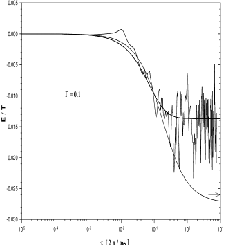
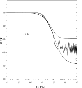
Figure 1: The formation of correlation energy due to molecular dynamic simulations [10] together with the analytical result of (LABEL:v2) for a plasma parameter $\Gamma=0.1$ (left) and $\Gamma=0.2$ (right). The upper curve is the static and the lower the dynamical calculation. The latter one approaches the Debye-Hückel result. The exact equilibrium correlation energy of MC simulations [11] are indicated by the arrow.

The explanation for this fact is that we can prepare the initial configuration within our kinetic theory such that sudden switching of interaction is fulfilled. However, in the simulation experiment we have initial correlations which are due to the setup within quasiperiodic boundary condition and Ewald summations. This obviously results into an effective statically screened Debye potential, or at least the simulation results allow for this interpretation.

If we go to higher densities of $\gamma=0.2$ in figure 1 (right) we see that the Debye Hückel result is far off the correct equilibrium correlation energy. Nevertheless the time scale is still appropriate described by the dynamical result. At still higher densities, like $\Gamma=0.5$ and $\Gamma=1$, see Fig. 2, non-ideal effects become important and the formation time is underestimated within (LABEL:v2). Of course, for higher plasma parameter the Born approximation fails. Nevertheless, formula (LABEL:v2) can still almost reproduce the formation time but slightly shorter than compared with the simulation. This is due to non-ideality which was found to be an expression of memory effects [12] and leads to a later relaxation. For strongly coupled plasma the Born approximation fails, of course, to reproduce the correct equilibrium value, but reproduces the formation time fairly good. The equilibrium value, of course, differs and takes smaller values than the Debye - Hückel result [11, 13]. This regime is clearly out of scope of our theory.

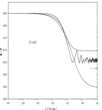
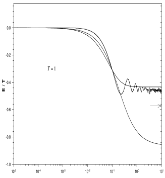
Figure 2: The formation of correlation energy due to molecular dynamic simulations [10] together with the result of (LABEL:v2) for a plasma parameter $\Gamma=0.5$ (left) and $\Gamma=1$ (right). The upper curve is the static and the lower the dynamical calculation. The latter one approaches the Debye - Hückel result. The simulation approaches the exact correlation energy [11] with higher densities indicated by the arrow.

The characteristic time of formation of correlations at high temperature limit is given by the time where (LABEL:v2) shows a saturation. This is reached at about a time of inverse plasma frequency

$$\tau_{c}\approx{1\over\omega_{p}}={\sqrt{2}\over v_{\rm th}\kappa}.$$ (14)

The inverse plasma frequency indicates that the dominant role is played by long range fluctuation. On the other hand, we also see that the correlation time is found to be given by the time a particle needs to travel through the range of the potential with a thermal velocity $v_{\rm th}$. This confirms the numerical finding of [3] that the correlation or memory time is proportional to the range of interaction, i.e. rather of short range character.

In the low temperature region, i.e., in a highly degenerate system $\mu\gg T$, one finds a different picture. From (6) follows [14]

$$E^{low}_{\rm corr}(t)-E_{\rm corr}^{low}(0)=E_{\rm corr}^{\rm low}{1-\frac{1}{x}\sin(x)+\left({2\mu\over\pi T}\right)^{2}\left(\frac{1}{3}+\left[\frac{1}{x}\sin(x)\right]^{\prime\prime}\right)\over 1+\frac{1}{3}({2\mu\over\pi T})^{2}}$$ (15)

with $x={4\mu\over\hbar}t$ and the equilibrium correlation energy

$$E_{\rm corr} = \frac{\mu e^{2}}{12\kappa^{3}\pi^{2}}\left(T^{2}+\frac{1}{3}\left({2\mu\over\pi}\right)^{2}\right)\left({m\over\hbar^{2}}\right)^{4}\left(\arctan{\frac{1}{b_{l}}}+{b_{l}\over 1+b_{l}^{2}}\right)$$

where the abbreviation is $b_{l}={\hbar\kappa\over 2p_{F}}$. We like to point out that the formula (15) is generally valid for any binary interaction and applicable in dense metal as well as nuclear situations. The only difference lies in the actual value of the equilibrium correlation energy which is dependent on the potantial, of course. Indeed, (15) follows from the standard procedure of separating angular from energy integrals for low temperatures. The time dependence is carried exclusively by the energy integrals while the angular averaged interaction results in its factor.

Unlike in the classical case, the equilibrium limit of the degenerate case (15) is not reached monotonously but with oscillation that are damped with power law $t^{-1}$ in time. In other words, the correlation energy is rapidly built up and then oscillates around the equilibrium value (LABEL:equil). We can define the build up time $\tau_{c}$ as the time where the correlation energy reaches its first maximum,

$$\tau_{c}=1.05{\hbar\over\mu}$$ (17)

with $\mu$ the Fermi energy. Note that $\tau_{c}$ is in agreement with the quasiparticle formation time known as Landau’s criterion. Indeed, as argued above, the quasiparticle formation and the build up of correlations are two alternative views of the same phenomenon.

The formation of binary correlations is very fast on the time scale of dissipative process. With respect to dissipative regimes, the binary correlations can be treated as instant functionals of the single-particle distribution and thus included into the Boltzmann equation via various renormalizations of its ingredients, would it be the screened Coulomb potential in the scattering rate or the quasiparticle corrections. Under extremely fast external perturbations, like the massive femto second laser pulses, the dynamics of binary correlations will hopefully become experimentally accessible. Even if related measurement will not reveal any unexpected features, the experimental justification of basic concepts of the non-equilibrium many-body physics is very desirable. The theoretical support to such experiments is mostly based on the non-equilibrium Green’s functions or the molecular dynamics which both demand expensive numerical treatments. Unlike these two approaches, the presented theory fails for special systems where the characteristic time of formation of correlations becomes longer or comparable with other time scales. For normal systems, it provides a simple tool for theoretical predictions.

We are grateful to G. Zwicknagel who was so kind as to provide the data of simulations. Stimulating discussion with G. Röpke is acknowledged. This project was supported by the BMBF (Germany) under contract Nr. 06R0884, the Max-Planck Society, Grant Agency of Czech Republic under contracts Nos. 202960098 and 202960021 and the EC Human Capital and Mobility Programme.

References

- [1] H. Haug and A. P. Jauho, Quantum Kinetics in Transport and Optics of Semiconductors (Springer, Berlin Heidelberg, 1996).
- [2] W. Theobald, R. Häßner, C. Wülker, and R. Sauerbrey, Phys. Rev. Lett. 77, 298 (1996).
- [3] M. Bonitz and et. al., J. Phys.: Condens. Matter 8, 6057 (1996).
- [4] P. Danielewicz, Ann. Phys. (NY) 152, 305 (1984).
- [5] H. S. Köhler, Phys. Rev. C 51, 3232 (1995).
- [6] K. Morawetz, Phys. Lett. A 199, 241 (1995).
- [7] K. Morawetz, Phys. Rev. E 50, 4625 (1994).
- [8] W. D. Kraeft, D. Kremp, W. Ebeling, and G. Röpke, Quantum Statistics of Charged Particle Systems (Akademie Verlag, Berlin, 1986).
- [9] J. Riemann and et. al., Physica A 219, 423 (1995).
- [10] G. Zwicknagel, C. Toepffer, and P. G. Reinhard, in Physics of strongly coupled plasmas, edited by W. D. Kraeft and M. Schlanges (World Scientific, Singapore, 1995), p. 45.
- [11] S. Ichimaru, Statistical Plasma Physics (Addison-Wesley Publishing company,, Massachusetts, 1994), p. 57.
- [12] K. Morawetz, R. Walke, and G. Röpke, Phys. Lett. A 190, 96 (1994).
- [13] H. DeWitt and et. al., Physica B 228, 21 (1996).
- [14] K. Morawetz and H. S. Koehler, Phys. Rev. C (1997), sub.