Noise Effects on Synchronized Globally Coupled Oscillators

Abstract

The synchronized phase of globally coupled nonlinear oscillators subject to noise fluctuations is studied by means of a new analytical approach able to tackle general couplings, nonlinearities, and noise temporal correlations. Our results show that the interplay between coupling and noise modifies the effective frequency of the system in a non trivial way. Whereas for linear couplings the effect of noise is always to increase the effective frequency, for nonlinear couplings the noise influence is shown to be positive or negative depending on the problem parameters. Possible experimental verification of the results is discussed.

Systems of coupled nonlinear oscillators are a generic paradigm of a whole class of problems arising in physics, chemistry, or biology [3]. Examples are Josephson Junction arrays (JJA) [4], charge-density waves [5], thin film fabrication [6], chemical reactions and cardiac tissue [7], neuronal activity [9], and many more (see, e.g., Ref. [3] and references therein). Due to the diversity of individual oscillators or to external (thermal) noise, these systems generally exhibit cooperative dynamical response or incoherent behavior as a function of the relevant parameters. The study of the transition between both regimes and the nature of the so-called synchronized phase requires the calculation of the phase distribution probability density. This involves solving a highly nonlinear, partial differential (Liouville) equation which is almost always a formidable task and only perturbative results can be obtained for practically all models of interest.

In this paper, we approach these problems by introducing a new method, from a completely different viewpoint, that avoids dealing with partial differential equations at all. We focus on the stochastic (Langevin) evolution equation that allows to perturbatively obtain accurate results in a very simple and direct manner. This method can be applied to any system of $N$ coupled homogeneous oscillators evolving in the presence of random forces, i.e., systems of the form

$$\dot{\phi}_{i}=\omega-f(\phi_{i})+\frac{\kappa}{N}\sum_{j=1}^{N}\Gamma(\phi_{i}-\phi_{j})+\sigma\eta_{i}(t),$$ (1)

where $\phi_{i}$ is the phase of oscillator $i$, $\omega>0$ is the oscillator frequency, $\kappa$ is a constant, $f(\phi)$ is any 2$\pi$-periodic function, $\Gamma$ is any separable (see below) function, and the random term $\eta_{i}$ is local (uncorrelated from site to site), Gaussian and stationary. Aside from these requirements, $\eta_{i}$ can be any process defined by a stochastic differential equation, e.g., it can be white or colored noise. To illustrate our method, we consider an Ornstein-Uhlenbeck process, given by $\dot{\eta}_{i}=-\gamma\eta_{i}+\gamma\xi_{i}(t)$, with $\xi_{i}(t)$ being uncorrelated Gaussian white noises [$\langle\xi_{i}(t)\xi_{j}(t^{\prime})\rangle=\delta_{ij}\delta(t-t^{\prime})$; $\langle\cdots\rangle$ stands for averages over noise realizations] and $\tau=1/\gamma$ being the correlation time.

Far from being academic, model (1) contains already several important applications. To begin with, the coupling can describe many different systems: For instance, in the case of the phase approximation of globally coupled nonlinear oscillators or of a JJA, $\Gamma(\phi_{i}-\phi_{j})=\sin(\phi_{i}-\phi_{j}+\alpha)$, $\alpha$ being a constant, whereas in reaction-diffusion (RD) problems such as those arising in growth models [6], the coupling comes from the discretization of some spatial linear operator followed by a mean field approximation, yielding $\Gamma(\phi_{i}-\phi_{j})=\phi_{i}-\phi_{j}$. Second, the nonlinear term, $f(\phi)$, for the oscillator can be chosen as required in each problem; as in most coupled oscillator models, we take here $f(\phi)=\sin\phi$, but our method can be applied to other choices as well.

We now begin the study of Eq. (1) in the case when, as mentioned above, $\Gamma$ is separable, i. e., $\Gamma(\phi_{j}-\phi_{i})=\sum_{n}A^{n}(\phi_{i})B^{n}(\phi_{j})$. This technicality is needed to simplify the study but does not not restrict much the applicability of our calculations. Eq. (1) becomes then

$$\dot{\phi}_{i}=\omega-f(\phi_{i})+\frac{\kappa}{N}\sum_{n}A^{n}(\phi_{i})\left[\sum_{j=1}^{N}B^{n}(\phi_{j})\right]+\sigma\eta_{i}(t).$$ (2)

The first step is to take the limit $N\to\infty$. In this limit the sum within the brackets above can be computed in terms of the mean value of $\phi$ [10]. As way of example, we focus on the RD problems and JJA’s, for which we arrive (respectively) at

$$\dot{\phi} = \omega-a\sin\phi+\kappa\left[\langle\phi\rangle-\phi\right]+\sigma\eta(t),$$ (3)

$$\dot{\phi} = \omega-a\sin\phi+$$ (5)

$$+\kappa\left[\cos(\phi-\alpha)\langle\sin\phi\rangle-\sin(\phi-\alpha)\langle\cos\phi\rangle\right]+\sigma\eta(t).$$

We note that we have thus reduced the $N$ equations in (1) to a single (self-consistent) one.

We deal first with eq. (3) for RD problems, hereafter called linear coupling model. When $\sigma=0$, it can be straightforwardly shown that if $\omega\leq\omega_{C}=a$ there is a stable time independent pinned solution $\phi=\sin^{-1}\omega/a$, whereas if $\omega>\omega_{C}$ the phase increases oscillatorily in time with frequency $\Omega^{2}\equiv\omega^{2}-a^{2}$. The natural question to ask is whether this scenario, involving a depinning transition at $\omega_{C}$, changes when noise is switched on, and if so, how. To address this issue we choose $\langle\phi\rangle$ as our order parameter, because in the pinned phase $\langle\phi\rangle$ is constant whereas in the depinned phase it increases in time. For noise intensities which are small compared to $\omega$ or $\kappa$, we expand $\omega_{C}$ and $\phi$ in powers of $\sigma$, $\omega_{C}=a+a^{(1)}\sigma+a^{(2)}\sigma^{2}+{\cal O}(\sigma^{3})$ and $\phi=\phi^{(0)}+\sigma\phi^{(1)}+\sigma^{2}\phi^{(2)}+{\cal O}(\sigma^{3})$. We first look for possible changes in $\omega_{C}$, by inserting these two expressions in Eq. (3); collecting powers of $\sigma$ and imposing that $\langle\dot{\phi}^{(i)}\rangle=0$ for $i=0,1,\ldots$ (i.e., that the oscillators remained pinned), we can compute the $a^{(i)}$ corrections to $\omega_{C}$. The final result is

$$\frac{\omega_{C}}{a} = 1-\frac{\sigma^{2}}{4\kappa(\kappa\tau+1)}+$$ (7)

$$+\frac{\sigma^{4}}{32\kappa^{4}}\left[\frac{\kappa^{2}-a^{2}}{(\kappa\tau+1)^{2}}+{\cal O}(\tau)\right]+{\cal O}(\sigma^{6}).$$

From this expression, we immediately see first, that the transition occurs at a value of $\omega$ which is lower than in the deterministic case, which means that the noise is actually helping the oscillators to overcome the barrier and start their motion. Another important conclusion is that for a given, fixed set of the other parameters, $\tau$ controls the state of the system: whereas for low $\tau$ values, the oscillators are depinned, as $\tau$ increases the pinned phase is set on. We thus see the importance of the correlation time in the critical region of the system.

Having found the changes in $\omega_{C}$, we now turn to the dynamics in the depinned phase, when $\omega>\omega_{C}$. We again expand $\phi$ in powers of $\sigma$ and write down equations for each contribution, which read

$$\langle\dot{\phi}^{(0)}\rangle = \omega-a\sin\langle\phi^{(0)}\rangle;$$ (9)

$$\langle\dot{\phi}^{(1)}\rangle = 0;$$ (10)

$$\langle(\dot{\phi}^{(1)})^{2}\rangle = -2\langle(\phi^{(1)})^{2}\rangle(\kappa+a\cos\langle\phi^{(0)}\rangle)+2\zeta(t),$$ (11)

$$\dot{\zeta} = \frac{\gamma}{2}-\zeta(\kappa+\gamma+a\cos\langle\phi^{(0)}\rangle);$$ (12)

$$\langle\dot{\phi}^{(2)}\rangle = -a\langle\phi^{(2)}\rangle\cos\langle\phi^{(0)}\rangle+a\frac{\langle(\phi^{(1)})^{2}\rangle}{2}\sin\langle\phi^{(0)}\rangle.$$ (13)

where $\zeta\equiv\langle\phi^{(1)}\eta\rangle$. Eq. (13) implies that $\langle\phi^{(2)}\rangle$ grows in time faster than $\langle\phi^{(0)}\rangle$, and therefore our expansion is not correct. This problem, very well known in deterministic equations [11], can be cured by realizing that the system dynamics does not depend only on one time scale but on two, $t$ and $t^{*}=\mu(\sigma)t$. Among the different approaches one can use to deal with this, we choose Linstedt’s method: we assume that $\phi^{(i)}$ depend on time through the combination $t+t^{*}$; as for $\mu(\sigma)$, dimensional analysis shows that the noise term is of order one when $\mu(\sigma)=\nu\sigma^{2}$. Introducing this new time scale in equations (9-13) and imposing the usual solvability condition on equation (13) (Fredholm’s alternative, see e. g. [11] for details) we obtain

$$\nu=\frac{a}{2T}\int_{0}^{T}\frac{\langle\phi_{1}^{2}\rangle\sin\langle\phi_{0}\rangle}{\omega-a\sin\langle\phi_{0}\rangle}dt,$$ (14)

where $T=2\pi/\Omega$ is the period of $\langle\dot{\phi}^{(0)}\rangle$ computed from eq. (9). With this value, the effective frequency of the oscillations, defined as $\omega_{\rm eff}=\lim_{t,s\to\infty}\frac{1}{s}[\langle{\phi}(t+s)\rangle-\langle{\phi}(t)\rangle]$, is:

$$\omega_{\rm eff}=\Omega(1+\nu\sigma^{2}+{\cal O}(\sigma^{4}))$$ (15)

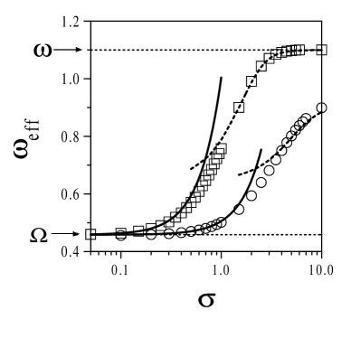
FIG. 1.: Predictions given by eqns. (15) up to order $\sigma^{2}$ (solid line) and (16) up to order $a^{2}$ (dashed line) are shown with the numerical solution of eqns. (3) for $N=5\,000$, $a=1$, $\kappa=1$, $\omega=1.1$ and $\tau=0$ (squares) or $\tau=10$ (circles). The numerical calculation was done with an explicit 2.0 order weak scheme [12].

Figure 1 compares our analytical, order $\sigma^{2}$ expression (15) for $\omega_{\rm eff}$ with the numerical solution of Eqs. (3) up to $\sigma\sim 0.5$, already a not so small value. The expression for $\omega_{\rm eff}$ above indicates that the noise increases the frequency as compared with the deterministic value, in agreement with our previous conclusion that the noise helps the oscillators jump over the potential barrier: The larger the noise strength, the easier the potential barrier to overcome, effectively suppresing (renormalizing) it in the $\sigma\to\infty$ limit. The fact that $\nu>0$, implying that the frequency increases with the noise strength, can be proven rigorously when $\tau=0$, i. e., for white noise, but we conjecture that this result is general for linearly coupled systems.

Another advantage of our approach is that it can be applied to other limits, such as the case when the noise intensity is larger than $\omega$ and $a$. Expanding the solution now in powers of $a$, the same steps as before yield, up to order $a^{2}$,

$$\omega_{\rm eff}=\omega-\displaystyle{a^{2}\over 2}\exp\left(-\frac{\tilde{\sigma}^{2}}{2\kappa}\right)\Bigg{[}\frac{\kappa^{2}\omega}{\kappa^{2}\omega^{2}+\omega^{4}}+$$ (16)

$$\displaystyle{\int}_{0}^{\infty}\exp\left\{{\frac{\tilde{\sigma}^{2}(\kappa\tau e^{-s/\tau}-e^{-\kappa s})}{2\kappa(\kappa\tau-1)}-\kappa s}\right\}\sin\omega s\ ds\Bigg{]}$$ (17)

where $\tilde{\sigma}=\sigma/\sqrt{\kappa\tau+1}$. Again, the comparison with the numerical solution (see Fig. 1) shows that our approach is very accurate, in this case for values of $\sigma$ down to $\sigma\sim 1.2$, very close to the values of $\omega$ and $a$. We want to stress that, except for a small interval $0.5\leq\sigma\leq 1.2$, our analytical predictions (15) and (16) describe to a high degree of accuracy the numerical solution for any noise intensity, providing a global picture of the main features of the linearly-coupled system behavior.

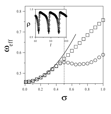
FIG. 2.: Comparison of the numerical values of $\omega_{\rm eff}$ for the linear (squares) and KS (circles) models with the small $\sigma$ approximation (15) (solid lines). Parameters are as in Fig. 1 with $\tau=0$. Note the synchronization-desynchronization transition for the KS model is at $\sigma\approx 0.5$. The inset shows the computed time evolution of the order parameter, $\rho$, (see text) in the KS model for $\sigma=0.2$ (circles) and the comparison with our analytical aproximation (solid line).

We now move on to the nonlinear problem (5) in the case $\alpha=0$; Eqs. (1) are then known as Kuramoto-Sakaguchi model (KS). In the small noise regime, our technique applied to the KS model leads once again to Eqs. (9-13). This stems from the fact that, when $\sigma\rightarrow 0$, the phases of individual oscillators are similar, and consequently $\sin(\phi_{j}-\phi_{i})\approx\phi_{j}-\phi_{i}$. However, due to the periodicity of the KS coupling term, the model is invariant under changes $\phi_{i}-\phi_{j}\leftrightarrow\phi_{i}-\phi_{j}+2n\pi$, for any integer $n$. Therefore, $2\pi$ jumps between oscillators are possible without consequence other than the breakdown of the linear approximation. Of course, the larger the noise strength, the more likely such jumps are, and the KS model becomes desynchronized at a finite value of $\sigma$, i. e., it has a true synchronization-desynchronization transition at $\sigma^{2}=\kappa$ when $a=0$ [3], and at lower values for $a\not=0$ [13]. Up to that point, it can be seen from Fig. 2 that the linear model, the KS model and our analytical prediction Eq. (15) are all in excellent agreement with each other. For our parameters, $a=1$, $\omega=1.1$, the transition takes place at $\sigma\approx 0.5$.

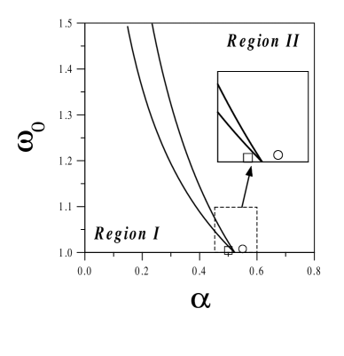
FIG. 3.: Diagram of the possible signs for $\nu(\alpha)$ for different values. Leftmost line corresponds to $\tau=10$, rightmost one to $\tau=0$. In both cases, Region I ($\nu_{\alpha}>0$) is ond the left of the line, Region II ($\nu_{\alpha}<0$) lies on the right. The square and the circle points correspond to the cases analyzed in figure (4).

The order parameter for the synchronization-desynchronization transition is $\rho=\langle\cos\phi\rangle^{2}+\langle\sin\phi\rangle^{2}$; in the synchronized phase, $\rho$ oscillates around a nonzero value, while in the desynchronized phase, $\rho=0$. The inset in Fig. 2 compares the numerical value of $r$ with the result of our aproximation, $\rho=1-\sigma^{2}\langle(\phi^{(1)})^{2}\rangle+{\cal O}(\sigma^{3})$, exhibiting the quantitative validity of our approach. The agreement is very good up to the critical value of $\sigma$. As for the limit $\sigma\to\infty$, the computations, although feasible, are quite involved, and therefore we do not present the results here.

In the two cases analyzed so far, in the synchronized phase noise helps the oscillators overcome the nonlinear potential, hence effectively increasing their frequency. However, this intuitively reasonable picture is not the generic situation: Antisymmetric couplings verifying $\Gamma(-\phi)=-\Gamma(\phi)$ keep the difference between oscillators small, forcing their motion to be approximately the same, and then the above picture holds, but if the coupling lacks this symmetry (like $\Gamma(\phi_{i}-\phi_{j}+\alpha)$ for nonzero $\alpha$), the oscillators do not tend to synchronize (they rather have phases separated by a factor $\alpha$). In the latter case, the noise competes with the frustration induced by the coupling and its activation effect disappears. Our calculations for Eqs. (5) when $\alpha\neq 0$ and $\sigma\to 0$ show that this is indeed what occurs. Our method leads now to a value of $\nu$, the $\sigma^{2}$ correction to the frequency, which depends on $\alpha$, given by

$$\nu_{\alpha}=\frac{1}{2T}\int_{0}^{T}\frac{\langle\phi_{1}^{2}\rangle(a\sin\langle\phi_{0}\rangle-2\kappa\sin\alpha)}{\omega_{0}-a\sin\langle\phi_{0}\rangle}\ dt$$ (18)

where $\omega_{0}\equiv\omega+\kappa\sin\alpha$, this parameter playing the role of an effective driving. Eq. (18) shows that, when $\alpha<\alpha_{0}\equiv\sin^{-1}(1/2\kappa)$, $\nu_{\alpha}$ is positive or negative depending on the value of $\omega$, whereas when $\alpha>\alpha_{0}$ we have $\nu_{\alpha}<0$. This divides the $(\omega,\alpha)$-space in two regions, according to the possible signs of $\nu_{\alpha}$, as depicted in Fig. 3. Interestingly, in region I $\alpha$ (or equivalently $\omega$) acts as a switching parameter between noise induced acceleration or deceleration of the oscillator motion, as illustrated in Fig. 4. Note that this is a novel, noise intrinsic phenomenon, absent in the deterministic problem, whose origin is the nonlinear coupling: If we add a constant to the coupling in Eq. (3) only the external frequency is changed ($\omega\rightarrow\omega+\kappa\alpha$).

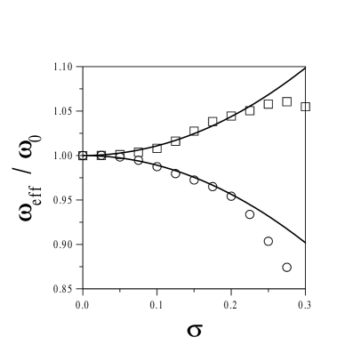
FIG. 4.: $\omega_{\rm eff}$ obtained from simulations for $\omega_{0}=1.006$, $\tau=0$, $\kappa=1$ and $\alpha=0.5$ (squares) or $\alpha=0.55$ (circles), compared to the analytical approximations (solid lines) given by eqns. (15) and (18). [Squares and circles refer to the corresponding points in Fig. 3].

In summary, we have introduced a procedure to study systems of globally coupled oscillators in the synchronized phase, general enough to analyze any stationary random processes generated by a stochastic differential equation, any form of the nonlinearity, and a large family of coupling terms. We have used it to analyze problems relevant in a number of physical contexts, obtaining fairly good results in a much more straightforward way than the approaches proposed so far. For linear coupling, we have computed the noise-induced corrections to the critical value for the depinning transition as well as the effective frequency in the depinned phase for almost all values of the noise. We have shown that the same results hold for the KS model. In the general case of frustrated JJA’s we have found that the effect of noise on the effective frequency is not trivial, leading to an increase or a decrease of the effective frequency depending on the system parameters and the driving frequency $\omega$. This very important result shows the power of our technique as it was not known prior to our work. Our predictions can be directly checked by experiments in very many fields, among which we suggest JJA’s subject to a magnetic field where tuning the voltage for a given temperature one should be able to find the two different behaviors predicted.

We are indebted to J. A. Cuesta and R. Cuerno for discussions. Work at GISC (Leganés) was supported by CICyT (Spain) grant MAT95-0325 and DGES (Spain) grant PB96-0119.

REFERENCES

- [1] Electronic address: eme@math.uc3m.es
- [2] Electronic address: anxo@math.uc3m.es
- [3] Y. Kuramoto, Chemical Oscillations, Waves, and Turbulence (Springer, Berlin, 1984); S. H. Strogatz, in Frontiers in Mathematical Biology, edited by S. Levin (Springer, Berlin, 1994).
- [4] A. V. Ustinov et al., Phys. Rev. B 47, 8357 (1993); S. Watanabe et al., Physica D 97, 429 (1996).
- [5] H. Fukuyama, J. Phys. Soc. Jpn. 41, 513 (1976); 45, 1474 (1978); H. Fukuyama and P.A. Lee, Phys. Rev. B 17, 535 (1977); P. A. Lee and T. M. Rice, Phys. Rev. B 19, 3970 (1979).
- [6] J. D. Weeks and G. H. Gilmer, Adv. Chem. Phys. 40, 157 (1979); A. Sánchez et al., Phys. Rev. B 51, 14 664 (1995); E. Moro et al., Phys. Rev. Lett. 78, 4982 (1997).
- [7] A. T. Winfree, When Time Breaks Down (Princeton University, Princeton, 1987).
- [8] C. W. Gardiner, Handbook of Stochastic Methods (Springer-Verlag, Berlin, 1996).
- [9] H. Sompolinsky et al., Phys. Rev. A 43, 6990 (1991).
- [10] When , the average of the phase over the ensemble of oscillators equals its average over realizations of the noise .
- [11] J. Kevorkian and J. D. Cole, Multiple Scale and Singular Perturbations Methods (Springer, New-York, 1996).
- [12] P. E. Kloeden and E. Platen, Numerical Solution of Stochastic Differential Equations (Springer, Berlin, 1992).
- [13] S. Shinomoto and Y. Kuramoto, Prog. Theor. Phys. 75 (1986), 1105.