Phase Diagram of Coupled Ladders

Abstract

The 2-leg $t$–$J$ ladder forms a spin liquid at half-filling which evolves to a Luther-Emery liquid upon doping. Our aim is to obtain a complete phase diagram for isotropic coupling (i.e. rungs and legs equal) as a function of electron density $n$ and the ratio $J/t$. Two known limiting cases are: $n<1/2$ which is a single band Luttinger liquid and small hole doping $\delta\ll 1$ for $J/t\longrightarrow 0$ which is a Nagaoka ferromagnet. Using Lanczos techniques we examine the region between the Nagaoka and Luther–Emery phases for $1>n>1/2$. We find evidences for gapless behavior in both spin and charge channels for $J/t<0.3$ consistent with Luttinger liquids in both bonding and anti-bonding bands (i.e., C2S2). This proposal is based on the behavior of spin and charge correlation functions. For example the hole–hole correlation function which displays hole pairing at larger $J/t$, shows hole–hole repulsion in this region. As a further test, we examined the dependence of the energy on a relative phase shift between bonding and antibonding bands. For $J/t<0.3$ this is very weak, indicating a lack of pairing between these channels.

I Introduction

The surprising discovery of high-$T_{c}$ materials by Bednorz and Müller [1] has sparked renewed interest in low-dimensional strongly correlated quantum systems. A striking feature of these materials is that they show simple long range antiferromagnetic (AF) order at low temperatures when they are not doped with holes.

Between the well-known one-dimensional systems and the difficult two dimensional system, coupled chains (or ladders) are interesting intermediate systems. The most striking feature of 2m-leg ladders is the appearance of a spin-gap at half-filling and small doping [2, 3, 4, 5, 6, 7, 8]. For instance compounds such as Sr_n-1Cu_n+1O_2n have been shown to be well described by a lattice of coupled $\nu_{n}$-leg ladders, with $\nu_{n}=(n+1)/2$ [9, 10]. Another example containing two-leg ladders is the system $\mbox{Sr}_{14-x}\mbox{Ca}_{x}\mbox{Cu}_{24}\mbox{O}_{41}$[11, 12] which is a material with doped ladders [13, 14] and where superconductivity (under high pressure) has been observed[15, 16, 17].

An important step is the determination of the phase diagram. Balents and Fisher [18] have computed the phase diagram of the Hubbard-ladder in the weak coupling limit $U\longrightarrow 0$ in the frame of bosonization and renormalization group theory. To distinguish the different phases they introduced the notation C$x$S$y$ for labeling phases with $x$ gapless charge and $y$ gapless spin excitations. Noack et al. [19] investigated then the different phases numerically with Density Matrix Renormalization Group (DMRG) methods for intermediate coupling and found good agreement with the analytical results of the weak coupling limit. The main feature is the existence of two regions, the Luther-Emery (LE) region with a spin gap (C1S0) and the Luttinger-Liquid (LL) with one gapless excitation (C1S1).

The strong coupling $t$–$J$ model [20, 21] has also been studied extensively by different authors. It is given by the Hamiltonian

$$H = t_{\perp}\sum_{j\sigma}\left(\tilde{c}^{{\dagger}}_{1j,\sigma}\tilde{c}_{2j,\sigma}+{\mathrm{h}.c.}\right)$$ (4)

$$+t_{\|}\sum_{lj\sigma}\left(\tilde{c}^{{\dagger}}_{lj+1,\sigma}\tilde{c}_{lj,\sigma}+{\mathrm{h}.c.}\right)$$

$$+J_{\perp}\sum_{j}\left({\mathbf{S}}_{1j}{\mathbf{S}}_{2j}-\frac{1}{4}n_{1j}n_{2j}\right)$$

$$+J_{\|}\sum_{lj}\left({\mathbf{S}}_{lj+1}{\mathbf{S}}_{lj}-\frac{1}{4}n_{lj+1}n_{lj}\right),$$

where the index $l\in\{1,2\}$ refers to legs and $j$ to rungs. The $\tilde{c}$ operators denote the fermion operators with projection onto the singly occupied states, i.e. $\tilde{c}_{lj,\sigma}=c_{lj,\sigma}(1-n_{lj,-\sigma})$. In this paper, we report a detailed study of the phase diagram for isotropic coupling (i.e. rungs and legs equal) as a function of electron density $n$ and the ratio $J/t$.

In the strong coupling limit $J_{\perp}\gg J_{\|}$, the spin-gap can be easily represented. At half-filling, the ground state is formed by spin-singlets lying on each rung. Turning over one spin gives a triplet on the corresponding rung. The energy difference between the two states, the spin-gap, is $\Delta\simeq J_{\perp}$. Numerically, it is found that the spin gap in the isotropic case $J_{\|}=J_{\perp}$ reduces to $\Delta\approx J_{\perp}/2$ [2, 3, 4]. The spin-gap of a doped ladder for $J_{\perp}\gg J_{\|}$ is due to a qualitatively different process. Some singlets have been replaced by hole-pairs moving along the ladder with a renormalized hopping $\widetilde{t_{\|}}$. The lowest excitation arises by breaking one hole pair (or equivalently a singlet bond) and putting each unbound spin on well-separated rungs. Turning over one of the separate spins gives the lowest triplet excitation with $\Delta\approx J_{\perp}-2t_{\perp}-2t_{\|}$ leading to a finite spin-gap (LE). At the isotropic point $J_{\perp}=J_{\|}$ and for $J/t\geq 0.3$ the spin-gap still exists where now the bound holes share neighboring rungs and strong singlet correlations are measured on the remaining sites [6, 22]. The spin-gap is thus a discontinuous function of doping in the vicinity of half-filling. For higher values of the parameter $J/t$, holes and electrons separate completely at all doping levels.

Thus, the appearance of the spin gap in a doped ladder is directly correlated with the formation of hole pairs, and it is an interesting problem to study their stability. Poilblanc et al. [23] used a numerical method based on Lanczos algorithms, which has allowed them to distinguish between the gapped and gapless regions in the phase diagram. Hayward and Poilblanc [24] determined the non-universal correlation exponents $K_{\rho}$ defining the behavior of the long-range correlations. They found at low electron density $n<1/2$ the system is in a LL phase, while for a higher electron density a gapped phase with hole pairs is stabilized. A large region of this gapped phase exhibits dominant superconducting correlations. The boundary of these two phases was determined to be $n\simeq 1/4$ where, in the band picture, the Fermi energy $E_{F}$ just touches the antibonding band.

However, some parts of the phase diagram are still unclear. First, the finite-size scaling process to determine the spin-gap region does not give clear results for values of $J/t<0.3$. Second, the radius of the hole pairs increases with decreasing $J/t$, and it is not clear whether it diverges for a particular value, and if a transition to a gapless phase occurs for small $J/t$. For very small values of $J/t$, the $t$–$J$ model is similar to the Hubbard model with $U\rightarrow\infty$. Since for two coupled chains, all spin configurations with a fixed $S_{z}$ are coupled by hole hopping as in a two-dimensional system, the essential condition for the Nagaoka theorem [26] is fulfilled. A ferromagnetic phase occurs for very small values of $J/t$ and low hole doping. In this phase, no spin gap occurs and holes repel each other. With increasing $J/t$, the ground state rapidly evolves into a singlet state.

This part of the phase diagram will be extensively studied on the basis of exact diagonalization results for small clusters, typically 10-rung ladders. Finite-size effects can be important for such systems, and it will be tried to minimize them as much as possible.

II Boundary Conditions

A Lanczos algorithm will be used to investigate the different phases. With current computers it is possible to investigate 2 leg ladders of length $L=10$ at any filling. In order to carry out a systematic analysis for different doping, the boundary conditions (BC) must be chosen carefully.

A Definition of Boundary Conditions

Usually, the BC are defined in the non-interacting limit of the model where the Hamiltonian is exactly described by two parallel bands $E_{\pm}(k)$ also labeled $E(k_{x},k_{y})$ with $k_{y}\in\{0,\pi\}$. Since the system is finite, the ${\mathbf{k}}(=(k_{x},k_{y}))$-values belong to a discrete set. In general $k_{x}=\frac{2\pi}{L}l+\phi$, where a priori $\phi$ needs not be the same for bonding ($k_{y}=0$) and antibonding ($k_{y}=\pi$) branches. BC giving either fully occupied or empty single particle orbitals in the non-interacting case, called closed shell (CS) boundary conditions (CSBC), are chosen.

If this condition is not fulfilled, the ground state is degenerate This favors the pairing of spins at $E_{F}$ and enhances pairing instabilities. This configuration is called open shell boundary conditions (OSBC).

The definition of the BC for the bonding and antibonding operators

$$b_{j\sigma} = \frac{1}{\sqrt{2}}(c_{1j,\sigma}+c_{2j,\sigma}),$$ (5)

$$a_{j\sigma} = \frac{1}{\sqrt{2}}(c_{1j,\sigma}-c_{2j,\sigma}),$$ (6)

are given by the set of equations (the spin index is droped for simplicity)

$$Tb^{{\dagger}}_{j}T^{-1} = e^{i\phi}b^{{\dagger}}_{j+1},\ \ \ 1\leq j<L,$$ (7)

$$Ta^{{\dagger}}_{j}T^{-1} = e^{i\phi}a^{{\dagger}}_{j+1},\ \ \ 1\leq j<L,$$ (8)

$$Tb^{{\dagger}}_{L}T^{-1} = e^{i\phi}b^{{\dagger}}_{1},$$ (9)

$$Ta^{{\dagger}}_{L}T^{-1} = e^{i(\phi+m\pi)}a^{{\dagger}}_{1}.$$ (10)

For $m=0$ the usual BC with the geometry of a ring are recovered. They will be generally referred to as RBC($\phi L$). $\phi L=0(\pi)$ are the most-used phases, which will be called periodic(antiperiodic) boundary condition or PBC(APBC). For $m=1$ the operators at the end of the legs fulfill the relationship

$$Tc^{{\dagger}}_{1\,L}T^{-1} = e^{i\phi}c^{{\dagger}}_{2\,1},$$ (11)

$$Tc^{{\dagger}}_{2\,L}T^{-1} = e^{i\phi}c^{{\dagger}}_{1\,1},$$ (12)

corresponding to the geometry of a Moebius band. They will be called Moebius Boundary Conditions and denoted by MBC$(\phi L)$. MBC($0$) means that periodic boundary conditions for bonding states and anti-periodic boundary conditions for antibonding states are taken and vice-versa for MBC($\pi$). In real space they can be viewed as a way to prevent antiferromagnetic frustration in some cases as schematically shown in Fig. 1 for a 10-rung ladder with two holes. For a phase differences $m\pi$ other than $0$ or $\pi$ the translation of one particle leads to two states, each one with one particle on each leg. This case will not be considered further.

By introducing these BC it is possible to get CSBC for all doping with an even number of holes. In the situation where two CSBC are possible, the one giving the minimal energy in the $t$–$J$ model will be generally preferred [25].

The Fourier transform

$$f_{k}=\sum_{{\mathbf{j}}}e^{i{\mathbf{k}}{\mathbf{j}}}f_{{\mathbf{j}}},$$ (13)

with ${\mathbf{k}}=(k_{x},k_{y})$ and ${\mathbf{j}}=(j_{1},j_{2})$ will be computed consistently by taking $k_{x}$ as a function of $k_{y}\in\{0,\pi\}$,

$$k_{x}(k_{y})=\left\{\begin{array}[]{ll}\frac{2\pi}{L}l&\mbox{RBC},\\[5.69054pt] \frac{2\pi}{L}l+\frac{\pi}{L}\delta_{k_{y},\pi}&\mbox{MBC},\end{array}\right.$$ (14)

where $l$ is an integer. The two possible sets of ${\mathbf{k}}$-values are summarized in Fig. 2.

III Nagaoka Phase

As discussed in the introduction, a Nagaoka phase [26] for $J/t\longrightarrow 0$ is expected at low doping. Numerically, Troyer [6] has shown that the ground state of $L\geq 4$-rungs $t$–$J$ ladders with a doping of two holes is a saturated ferromagnet at $J/t=0.$ In the following, the doping and $J/t$ dependence of this phase will be investigated.

The analysis of that phase is simplified by first considering the subspace of the completely polarized states ($S_{z}^{tot}=N_{s}/2$ with $N_{s}$ the number of spins) which is equivalent to a spinless fermion system. The eigenvalues are exactly given by the band picture $E_{\pm}({\mathbf{k}})=-2t_{\|}\cos(k_{x})\pm t_{\perp}$ and the eigenstates are direct products of bonding and antibonding states. For finite clusters CSBC can be sometimes obtained with different BC. For instance, for a 10-rung ladder with 2 holes and with $t_{\perp}=t_{\|}$ both APBC and MBC($0$) allow a CS configuration with the same ground state energy as schematically plotted in the upper graphs of Fig. 3. For higher $J/t$, when the ground state is a singlet, the corresponding CSBC configurations are shown in the lower graphs of Fig. 3 where black circle stand for fully occupied states. Both MBC($0$) and MBC($\pi$) are possible.

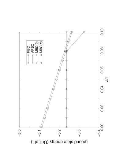
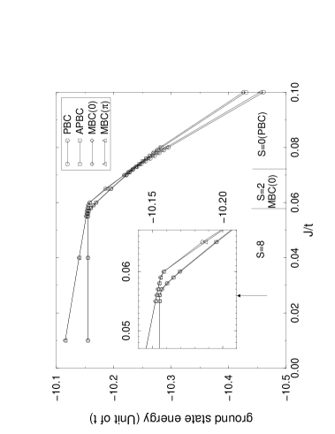
In Fig. 4 and 5 the ground state energy is shown for different cases. In Fig. 4 the upper graph shows the lowest energies for a 5-rung ladder with one hole and the lower graph for a 10-rungs ladder with two holes. In Fig. 5 the lowest energies for a 5-rung ladder with two holes and for a 10-rung ladder with four holes is shown in the upper and lower graph, respectively. Each curve corresponds to different BC. For each graph, the transition to the saturated ferromagnet where the energy is $J/t$-independent is clearly seen for CSBC. The two other BC do not have CS and the corresponding energy states are singlets showing a linear $J/t$-dependent energy lying above the energy of the fully polarized state. This case will not be considered further.

A crude finite size scaling can be made by extrapolating the critical values of a 5-rung and a 10-rung ladder[24]. At a doping of $\delta=0.1$, for $L=5$ the lowest critical value is given by APBC with value $(J/t)_{5}\simeq 0.052$ while for $L=10$ both APBC and MBC($0$) gives the same critical value of $(J/t)_{10}\simeq 0.042$. The infinite extrapolation gives $(J/t)_{\infty}\simeq 0.032$. For $\delta=0.2$, the two values are $(J/t)_{5}\simeq 0.078$ and $(J/t)_{10}\simeq 0.056$ respectively, and the infinite extrapolation gives $(J/t)_{\infty}\simeq 0.034$. For higher doping, i.e. for a 5-rung ladder with three holes and for a 10-rung ladder with five and six holes with $J/t\geq 0$ no ferromagnetic ground state has been found.

In conclusion the diagonalization of small clusters shows signs of saturated ferromagnetism up to a doping of $\delta\simeq 0.2$ and for small values of $J/t$ ($J/t\simeq 0.033$).

A For $J/t>(J/t)_{\textrm{f}}$, Sign of Partial Ferromagnetism?

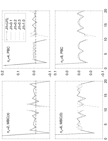
For some clusters, the transition from the Nagaoka phase to the singlet phase does not occur immediately, but passes through different phases with an intermediate spin $0<S<N_{e}/2$. The lowest energy of the $n_{\mathrm{h}}=2$, $10$-rung ladder for $J/t<0.09$ is always given by APBC (with the exception of a very tiny region close to $J/t=0.04$). In that region, the spin of the corresponding ground state passes through the finite values $S=5$ for $0.043\leq J/t\leq 0.057$ and $S=1$ for $0.058\leq J/t\leq 0.062$. For $J/t>0.62$ the ground state is a singlet with a finite momentum of $k=\pi/5$ and a singlet at zero momentum for $J/t\geq 0.083$; they are mentioned at the bottom of Fig. 4. For a 10-rung ladder with $n_{\mathrm{h}}=4$ (Fig. 5), some partial ferromagnetism also occur. For $0.057\leq J/t\leq 0.072$ the spin is $S=2$ with MBC$(0)$ giving the lowest energy. For $J/t>0.072$, the lowest energy is given by PBC at $k_{x}=0$ and is a singlet.

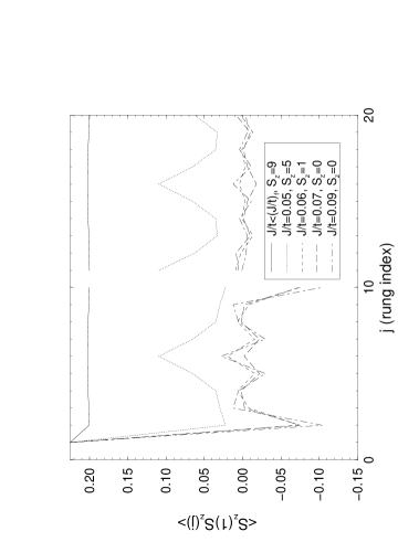
The spin–spin correlations for the 10-rung ladder with $n_{h}=2$ and for $S_{z}=S$ are plotted in Fig. 6. The correlations in real space are plotted in the uppermost graph where the sites on the first leg are labeled $1\leq j\leq 10$, and on the second leg $11\leq j\leq 20$ as pictured in Fig. 1. For $J/t\geq 0.05$, they show an alternating behavior around a ferromagnetic value indicating antiferromagnetic correlations. However, their Fourier transform, plotted in the lower graph, do not clearly indicate a continuous process. For $J/t=0.07$ the correlation functions have a maximum in the branch $k_{y}=\pi$ indicating that the sum of the interband scattering processes is greater than the intraband processes and thus, that the correlations between both bands are important. The correlations at other values of $J/t$ display a maximum in the $k_{y}=0$ branch showing that the intraband processes are now favored.

These effects are not found for small systems (L=5). It is thus tempting to conclude the existence of narrow region with partial ferromagnetism phase in the thermodynamic limit of the $n$–$J$ phase diagram. However the present results are not enough to draw a clear conclusion on this subject and the existence of these phases is still open.

IV Existence of a C2S2 Region?

The spin gap of a doped system is intrinsically bound to the formation of hole pairs. Moreover, it is known that for very low $J/t$, when the system is ferromagnetic, holes repel each other. The question of whether the transition between repulsive and attractive holes occurs at the ferromagnetic to paramagnetic transition will be addressed in this section. Numerical evidence shows that a region of holes with repulsive residual interactions, and thus with gapless spin excitations, occurs between the ferromagnetic and the LE phase.

A Hole–Hole Correlations

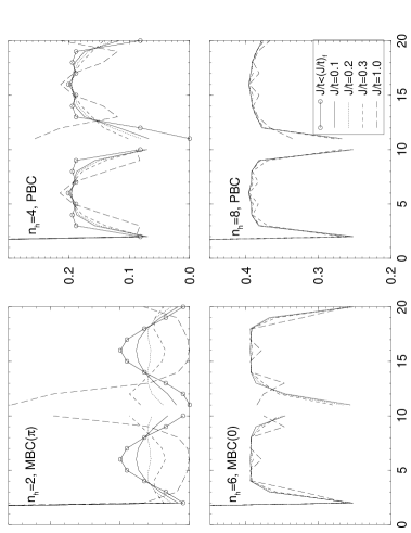
A first insight into this question can be obtained by looking at the hole–hole correlation function $\langle n_{\mathrm{h}}(1)n_{\mathrm{h}}(j)\rangle$. In Fig. 7 the correlations are plotted for different values of $J/t$ and different fillings, namely $n_{\mathrm{h}}=2$ with MBC$(\pi)$, $n_{\mathrm{h}}=4$ with PBC, $n_{h}=6$ with MBC$(0)$ and $n_{\mathrm{h}}=8$ with PBC [27]. For $n_{\mathrm{h}}=2$ and $n_{\mathrm{h}}=4$ the correlation for the ferromagnetic state computed with APBC is also shown (circles). The uppermost graphs in the figure show the correlation functions in real space with the site convention pictured in Fig. 1. Each correlation is normalized such that $\mbox{$\langle n_{\mathrm{h}}(1)n_{\mathrm{h}}(1)\rangle$}=1$.

The lower graphs show the Fourier transform

$$\mbox{$\langle n_{\mathrm{h}}(k)n_{\mathrm{h}}(-k)\rangle$}\propto{\cal N}({\mathbf{k}})\equiv\sum_{{\mathbf{j}}}e^{i{\mathbf{k}}{\mathbf{j}}}\mbox{$\langle n_{\mathrm{h}}(1)n_{\mathrm{h}}({\mathbf{j}})\rangle$},$$ (15)

where ${\mathbf{k}}$ is defined in Sec. II. The normalization corresponds to ${\cal N}(0)=n_{\mathrm{h}}$ (out of the graphs). In Fourier space, the points in the $k_{y}=0(\pi)$ branch are given by the left(right) curves in each graph.

In real space, each graph shows the same behavior. For instance for $n_{h}=2(\delta=0.1)$ at $J/t=0.1$ the second hole is found to sit at the farthest point from the first hole. When $J/t$ is increased the hole–hole correlation for having two holes on the same rung increases. When $J/t=1$ the hole–hole correlation clearly shows their bound character.

In the large $J_{\perp},t_{\perp}$ limit, with $J_{\perp}>2t_{\perp}$, the hopping of hole pairs between rungs is given in second order perturbation theory by $\widetilde{t_{||}}=-2t_{||}^{2}/(J_{\perp}-2t_{\perp})$. As the hole pairs act as hard-core bosons, they repel each other in order to gain the maximal kinetic energy. This can be viewed in the lower graphs plotting the Fourier-transform, where peak in the $k_{y}=0$ branch appear. This feature clearly appears in the four different graphs. At the same time, the total weight in the $k_{y}=\pi$ decreases.

This behavior raises the question of the existence of an intermediate phase below the LE phase. In fact, for two holes and values of $0.05<J/t<0.2$ the system seems to be in a phase where holes repel each other. According to the above picture, it would imply spin-gapless excitations. However, it could also be a pure finite size effect in that the radius of a two-hole bound state is greater than the length of the ladder sample. Thus, finite size effects strongly complicate the interpretation. The above correlations are not enough to conclude definitively to the existence of a new phase.

B Spin–Spin Correlations

The spin–spin correlation of the systems are plotted in Fig. 8. The uppermost graphs show the spin-spin correlations $\langle S_{z}(1)S_{z}(j)\rangle$ in real space. They clearly show the antiferromagnetic ordering of the spins along the chain. For $n_{\mathrm{h}}=4$ and $n_{\mathrm{h}}=6$ and for low value of $J/t$, the correlation across the rung $\langle S_{z}(1)S_{z}(11)\rangle$ is ferromagnetic not antiferromagnetic. Increasing $J/t$ however stabilizes the system to have antiferromagnetic ordering across the rung.

This feature is also clearly emphasized by the Fourier transform, plotted in the lower graph of Fig 8, which have their maxima in the $k_{y}=0$ branch. Their Fourier transforms ${\cal M}({\mathbf{k}})$ also gives information on the different scattering processes occurring between the different spins in the band picture. In fact, they are proportional to the equal-time correlation function,

$${\cal M}({\mathbf{k}})\propto\mbox{$\langle S_{z}(k)S_{z}(-k)\rangle$}=\sum_{\mbox{$|\alpha\rangle$}}|\mbox{$\langle\alpha|S_{z}(k)|0\rangle$}|^{2},$$ (16)

where the sum is taken over all eigenstates of $H$ and where $|0\rangle$ denotes the ground state. For the case $n_{\mathrm{h}}=2$, the MBC($\pi$) has bonding states filled up to $k_{\mathrm{F,b}}=\frac{\pi}{2}$ and antibonding to $k_{\mathrm{F,a}}=\frac{\pi}{5}$ as schematically shown in Fig. 3. The lowest energy intraband excitations in the bonding and antibonding band occur at ${\mathbf{k}}_{b}=(2k_{\mathrm{F,b}}+\frac{2\pi}{L},0)=(\frac{6\pi}{5},0)$ and at ${\mathbf{k}}_{a}=(2k_{\mathrm{F,a}}+\frac{2\pi}{L},0)=(\frac{3\pi}{5},0)$, respectively. The corresponding curves in Fig. 8 show a maximum at ${\mathbf{k}}_{b}$ while no peak appear at ${\mathbf{k}}_{a}$ showing that these processes do not dominate in the sum of Eq. 16. Moreover, these processes are quite small compared to the interband processes plotted in the right part of the graph. According to the band picture the lowest energy interband processes are at ${\mathbf{k}}_{ab}=(k_{\mathrm{F,b}}+k_{\mathrm{F,a}}+\frac{\pi}{L}=\frac{9\pi}{10},\pi)$. The curve display a maximum at that point dominating all the other processes and especially the intraband scattering ones. It leads to the interpretation that the bonding and antibonding particles are strongly correlated at $E_{F}$. In the next section a picture will be proposed in which the gapless phase is a manifestation of the absence of correlation between bands. In such a picture, the correlation for $n_{\mathrm{h}}=2$ is characteristic for a gapped phase.

For $n_{\mathrm{h}}=4$(PBC) the band picture in the non interacting limit predicts dominant intra-bonding band scattering processes at ${\mathbf{k}}_{b}=(\pi,0)$ and intra-antibonding band scattering processes at ${\mathbf{k}}_{a}=(3\pi/5,0)$. Dominant interband scattering processes occur at ${\mathbf{k}}_{ab}=(4\pi/5,\pi)$. These values correspond to the (local)maxima of the correlation in agreement with the simple non-interacting band picture.

For $n_{\mathrm{h}}=6$(MBC($0$)) the dominant scattering processes are expected at ${\mathbf{k}}_{b}=(\pi,0)$, ${\mathbf{k}}_{a}=(2\pi/5,0)$, and ${\mathbf{k}}_{ab}=(7\pi/10,\pi)$. For $n_{\mathrm{h}}=8$(PBC) the dominant scattering processes are expected at ${\mathbf{k}}_{b}=(\pi,0)$, ${\mathbf{k}}_{a}=(\pi/5,0)$, and at ${\mathbf{k}}_{ab}=(3\pi/5,\pi)$. The corresponding graphs display corresponding maxima in good agreement with the band-picture predictions.

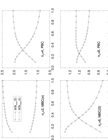
In Fig. 9 the maxima of the correlation functions for the $k_{y}=0$(circle) and the $k_{y}=\pi$(square) branches are plotted. For $n_{\mathrm{h}}=4,6$ and $n_{\mathrm{h}}=8$ they show a crossover from a region with dominant intraband scattering to a region with dominant interband scattering. This suggests that the system has uncorrelated bonding and antibonding bands at $E_{F}$ such that the low energy physics is analogous to that of two one-dimensional systems, with spin and charge gapless excitations (C2S2). A rough criteria for the transition can be defined by taking the critical $J/t$ at the crossover. This yields $(J/t)_{\mathbf{c}}\simeq 0.32,0.34,0.26$ for $\delta=0.2,0.3$, and $\delta=0.4$, respectively. For $n_{\mathrm{h}}=2$ the interband scattering is always much bigger than the intraband scattering yielding to the conclusion that no C2S2 phase occurs for that particular filling. This emphasizes that care must be taken in interpreting the simple hole–hole correlations.

C (Anti-) Bonding Pair Correlations

Defining the singlet $\hat{S}^{{\dagger}}_{i}$ and triplet $\hat{T}^{{\dagger}}_{i0}$, $\hat{T}^{{\dagger}}_{i\alpha}$, $\alpha\in\{\uparrow,\downarrow\}$ creation operator on the rung $i$ with

$$\hat{S}^{{\dagger}}_{i} = \frac{1}{\sqrt{2}}(c^{{\dagger}}_{1i\uparrow}c^{{\dagger}}_{2i\downarrow}-c^{{\dagger}}_{1i\downarrow}c^{{\dagger}}_{2i\uparrow}),$$ (17)

$$\hat{T}^{{\dagger}}_{i0} = \frac{1}{\sqrt{2}}(c^{{\dagger}}_{1i\uparrow}c^{{\dagger}}_{2i\downarrow}+c^{{\dagger}}_{1i\downarrow}c^{{\dagger}}_{2i\uparrow}),$$ (18)

$$\hat{T}^{{\dagger}}_{i\alpha} = c^{{\dagger}}_{1i\alpha}c^{{\dagger}}_{2i\alpha},$$ (19)

the different pair correlations between bonding and antibonding states in the subspace of single occupied states can be written as [28]

$$\begin{array}[]{lcr}\mbox{$\langle b^{{\dagger}}_{i\uparrow}b^{{\dagger}}_{i\downarrow}a_{j\uparrow}a_{j\downarrow}\rangle$}&=&\frac{1}{2}\mbox{$\langle\hat{S}^{{\dagger}}_{i}\hat{S}_{j}\rangle$},\\[5.69054pt] \mbox{$\langle b^{{\dagger}}_{i\uparrow}a^{{\dagger}}_{i\downarrow}b_{j\uparrow}a_{j\downarrow}\rangle$}&=&-\frac{1}{2}\mbox{$\langle\hat{T}^{{\dagger}}_{i0}\hat{T}_{j0}\rangle$},\\[5.69054pt] \mbox{$\langle b^{{\dagger}}_{i\alpha}a^{{\dagger}}_{i\alpha}b_{j\beta}a_{j\beta}\rangle$}&=&-\mbox{$\langle\hat{T}^{{\dagger}}_{i\alpha}\hat{T}_{j\beta}\rangle$}.\end{array}$$ (20)

In the C2S2 phase, when the bonding and antibonding states are not correlated, all pair correlations are shortrange. In the spin-gapped region, the ground state is characterized by the formation of interchain singlet. Thus, long range singlet-singlet (SS) pair correlations will appear while the triplet–triplet (TT) pair correlations will remain short-range.

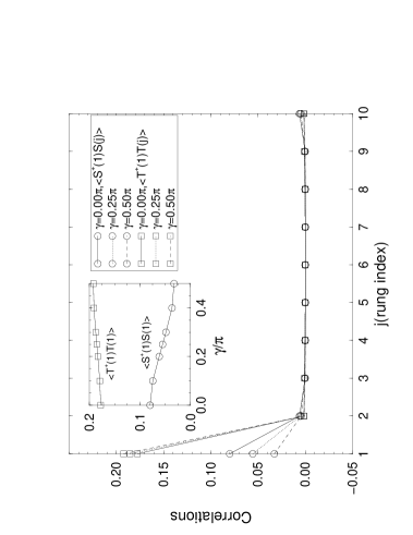
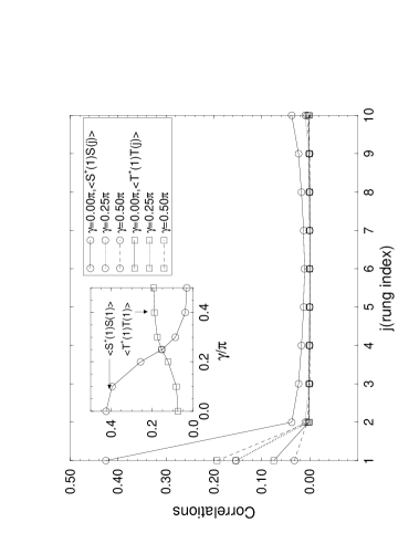
For an undoped system, the pair correlations are finite only on the same rung $j=i$, where they are proportional to the number operator for singlet or triplet states, and depend only on the ratio $J_{\perp}/J_{\|}$. For $J_{\|}=0$, the singlet–singlet pair correlation at $j=i$ is 1 while the triplet–triplet pair correlation at $j=i$ is 0. At the isotropic point, the values for the undoped 10-rung ladder are

$$\langle\hat{S}^{{\dagger}}(1)\hat{S}(1)\rangle \simeq 0.7,$$ (21)

$$\langle\hat{T}_{0}^{{\dagger}}(1)\hat{T}_{0}(1)\rangle = \mbox{$\langle\hat{T}_{\uparrow}^{{\dagger}}(1)\hat{T}_{\uparrow}(1)\rangle$}\simeq 0.1.$$ (22)

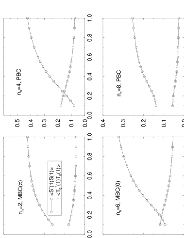
In a doped system, the pair correlations at the isotropic point depend on the ratio $J/t$. In Fig. 10 $\langle\hat{S}^{{\dagger}}(1)\hat{S}(1)\rangle$ and $\langle\hat{T}_{0}^{{\dagger}}(1)\hat{T}_{0}(1)\rangle$ are plotted as function of $J/t$. The case $n_{\mathrm{h}}=2$ shows that $\mbox{$\langle\hat{S}^{{\dagger}}(1)\hat{S}(1)\rangle$}>\mbox{$\langle\hat{T}_{0}^{{\dagger}}(1)\hat{T}_{0}(1)\rangle$}$ for all plotted values $J/t$. It favors the scenario that a 10-rung ladder with two holes has a gap for very low $J/t$-values in agreement with the discussion of the spin–spin correlation. With increasing $J/t$ the singlet number $\langle\hat{S}^{{\dagger}}(1)\hat{S}(1)\rangle$ rapidly increases while the triplet number $\langle\hat{T}_{0}^{{\dagger}}(1)\hat{T}_{0}(1)\rangle$ decreases. On contrary, for $n_{\mathrm{h}}=4(6)$ a cross-over between the singlet and triplet number occurs at $J/t\simeq 0.23(0.17)$. This is in agreement with the speculated gapless region at low $J/t$. The case with $n_{\mathrm{h}}=8$, exhibits a favored rung singlet configuration.

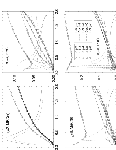
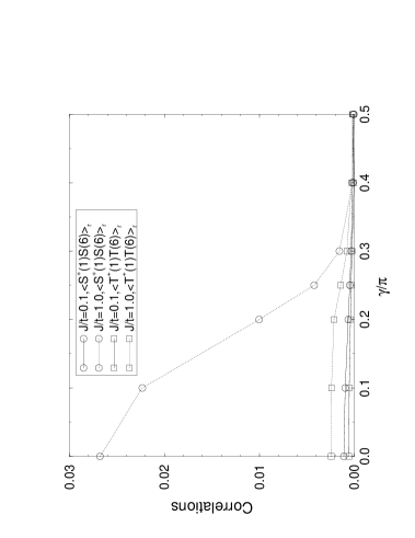
In Fig. 11 the pair correlation at different rungs is shown as a function of $J/t$ for the different cases. To make a consistent comparison of the long-range order for various $J/t$ the pair correlations are normalized according to the singlet number, $\mbox{$\langle\hat{S}^{{\dagger}}(1)\hat{S}(j)\rangle$}_{r}=\mbox{$\langle\hat{S}^{{\dagger}}(1)\hat{S}(j)\rangle$}/\mbox{$\langle\hat{S}^{{\dagger}}(1)\hat{S}(1)\rangle$}$. For $n_{\mathrm{h}}=2$ the pair correlations uniformly tend to zero when $J/t$ decreases to zero. The solid and dotted lines show the derivative (forward difference) of the curves for $j=2$ and $j=3$. Both show a peak around $J/t=0.3$ indicating the value of $J/t$ below which the pair correlation become short-ranged. The curve does not show any different behavior for $J/t>0.1$. Below this value, it has been seen that the system has a transition to a ferromagnetic phase at $J/t=0.032$. Between these two points some sign of partial ferromagnetism has been discussed but no direct evidences for a C2S2 phases has been observed.

The striking feature of the graphs for $n_{\mathrm{h}}=4,6$ and $n_{\mathrm{h}}=8$ is the qualitatively different behavior of the different curves at small $J/t$. The normalized short range pair correlation $\mbox{$\langle\hat{S}^{{\dagger}}(1)\hat{S}(2)\rangle$}_{r}$ shows a minimum at $J/t=0.30,0.45$, and $0.50$ for $n_{\mathrm{h}}=4,6$, and $8$, respectively. The solid and dashed/dotted lines show the derivative of the different curves. Maxima in the derivatives appear in both cases for $0.25<J/t<0.5$ below which value the correlation get short range.

A critical value will be defined to be at the point where the long-range pair correlation $\mbox{$\langle\hat{S}^{{\dagger}}(1)\hat{S}(5)\rangle$}_{r}$ change the slope of its curve. This gives the values $(\widetilde{J/t})_{\mathbf{c}}\simeq 0,20,0.25,0.25$ for $\delta=0.2,0.3$, and $0.4$, respectively.

V Transformed Hamiltonian

In this section, the physical picture for the C2S2 phase based on the absence of phase correlation between the bonding and anti-bonding bands is examined. For $J/t\simeq 0.5$ phase coherence between the bands at $E_{F}$ exists leading to a LE liquid with the spingap. The question whether this phase coherence disappears for small $J/t$ leading to two independent LL (C2S2) will be investigated [29]. The terms in the Hamiltonian coupling both bands are of the form $b_{k_{1},\sigma}^{{\dagger}}b_{k_{2},\sigma^{\prime}}^{{\dagger}}a_{k_{3},\sigma^{\prime}}a_{k_{4},\sigma}+{\mathrm{h}.c.}$. They must be irrelevant near $E_{F}$ in the gapless LL phase and become relevant when $J/t$ increases. To investigate this we transform the Hamiltonian by introducing a relative phase between the bonding and antibonding operators, so that only terms of the above form are affected, then the dependence of the ground state on this phase difference will be studied.

A Relative Phase Transformation

The transformation is defined by

$$H=PH(b,a)P\rightarrow PH(e^{i\phi_{b}}b,e^{i\phi_{a}}a)P=H_{\mathrm{t}},$$ (23)

where $P$ is the projector onto singly occupied states and $H(a,b)$ is the $t$–$J$ Hamiltonian (without projection) written in the bonding and antibonding basis. The hopping term of the Hamiltonian is diagonal in the bonding and antibonding basis and thus does not change. The introduction of a phase shift will only affect terms of the form

$\displaystyle b^{{\dagger}}b^{{\dagger}}aa\rightarrow e^{i2(\phi_{b}-\phi_{a})}b^{{\dagger}}b^{{\dagger}}aa,$

which occur in the $H_{J_{\|}}$ and $H_{J_{\perp}}$ part. They couple the bonding and the antibonding operators and are thus responsible for the appearance of the spin gap.

With $\gamma=\phi_{b}-\phi_{a}$, The total transformation is summarized through the definition,

$$PH(c_{lj})P\longrightarrow PH(c_{lj,\mathrm{t}})P=H_{\mathrm{t}}(\gamma),$$ (24)

where the transformed Hamiltonian $H_{\mathrm{t}}(\gamma)$ has a periodicity of $\pi$ in $\gamma$. The site operators are transformed according to the rule $c_{lj}\longrightarrow c_{lj,\mathrm{t}}$ with

$$c_{1j,\mathrm{t}} = \frac{1}{2}\left((e^{i\phi_{b}}+e^{i\phi_{a}})c_{1j}+(e^{i\phi_{b}}-e^{i\phi_{a}})c_{2j}\right)$$ (25)

$$c_{2j,\mathrm{t}} = \frac{1}{2}\left((e^{i\phi_{b}}-e^{i\phi_{a}})c_{1j}+(e^{i\phi_{e}}+e^{i\phi_{a}})c_{2j}\right).$$ (26)

The final transformed Hamiltonian can be written with three distinct terms

$\displaystyle H_{\mathrm{t}}=H_{\mathrm{t},h}+H_{\mathrm{t,J_{\|}}}+H_{\mathrm{t,J_{\perp}}},$

where the first part $H_{\mathrm{t},h}$ is the hopping part being the same as in the original Hamiltonian. The second term $H_{\mathrm{t,J_{\|}}}$ involving magnetic coupling along the chain contains four distinct terms

$$H_{\mathrm{t},J_{\|}} = H_{\mathrm{t,J_{\|},1}}+H_{\mathrm{t,J_{\|},2}}+H_{\mathrm{t,J_{\|},3}}+H_{\mathrm{t,J_{\|},4}}$$ (27)

which are listed and discussed in Appendix A. The interleg magnetic coupling $H_{\mathrm{t},J_{\perp}}$ vanishes at $\gamma=\pi$ (see Appendix A) in agreement with the suppression of correlation between the bonding and antibonding operators.

B Ground State Energy

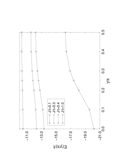
The ground state may not be completely decoupled into a bonding and an antibonding part. Only the particles with a $k$-value near $E_{F}$ must be uncorrelated for two independent LL. By calculating the ground state energy of $H_{\mathrm{t}}$ the influence of the phase shift on all bonding and antibonding operators is included and it is thus possible that the influence of the phaseshift is qualitatively similar for different values of $J/t$. In fact, in Fig. 12 the ground state energy is plotted for a 10-rung ladder with 4 holes and using PBC. By switching on $\gamma$, the energy increases for all plotted values of $J/t$. However, no clear qualitative change in the evolution of the energy vs $\gamma$ for different $J/t$ can be observed. This is a consequence of the fact that all particles (also away from $E_{F}$) are involved. It is interesting to consider the different correlation functions to look for signs if the system undergoes a phase-transition when $\gamma$ is altered.

C Correlation Functions

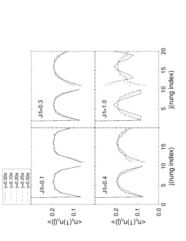
In Fig. 13 the hole–hole correlations for a 10-rung ladder with 4 holes are plotted. The correlations are shown at different $J/t$ for different values of $\gamma$. The upper graphs show the correlations in real space, and the lower their Fourier transform. For $J/t\leq 0.3$ only small changes in the shape of the correlations are observed when $\gamma$ increases. For $J/t=0.4$ and $J/t=1.0$ the shape of the correlation is clearly changed indicating state with repulsive interactions at $\gamma=0.5\pi$. The influence of $\gamma$ for $J/t=1.0$ is the most important. The rung correlation $\langle n_{\mathbf{h}}(1)n_{\mathbf{h}}(11)\rangle$ is clearly suppressed in agreement with the breaking of hole-pairs. The diagonal correlation $\langle n_{\mathbf{h}}(1)n_{\mathbf{h}}(12)\rangle$ shows a peak at $\gamma=0.2\pi$ which is suppressed for $\gamma=0.5\pi$. The peak in the branch $k_{y}=0$ of the Fourier transform, characteristic of the homogeneity of the hole-pair repartition is also suppressed.

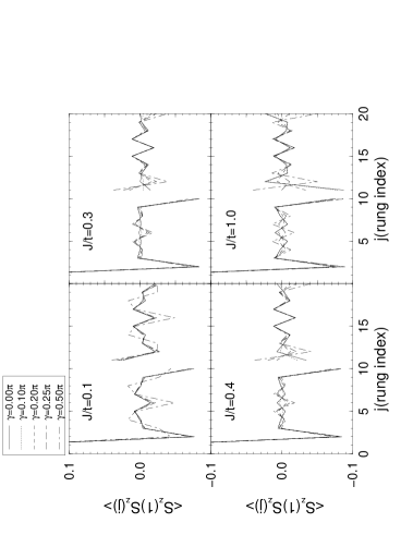
In Fig. 14 the spin–spin correlation for the same cluster is plotted. The measured antiferromagnetism is quite sensitive to the phase shift. In real space the antiferromagnetic correlation across the rungs is turned into leg independent behavior (rung ferromagnetism). However, ${\cal M}({\mathbf{k}})$ measures all spins in the band pictures, therefore not only those at $E_{F}$, and a change in the correlation is also compatible with the gapless phase. The most striking picture of the spin–spin correlations is given by their Fourier transforms. As discussed above, dominant peaks in the bonding channel ($k_{y}=0$) are expected for the gapless phase, while dominant interband ($k_{y}=\pi$) scattering processes are expected in the gapped phase. This behavior appears clearly in all graphs.

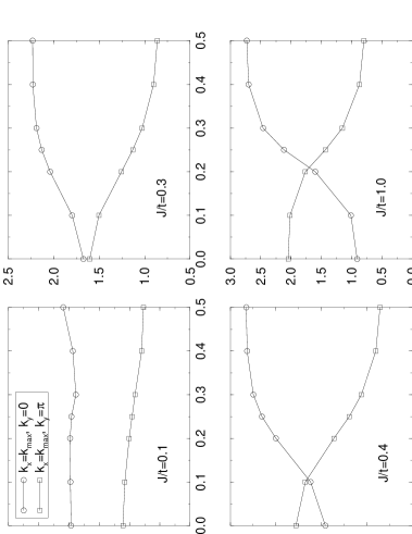
In Fig. 15 the maxima of the spin–spin correlations as a function of $\gamma$ are shown for the different $J/t$ values. They are at ${\mathbf{k}}=(\pi,0)$(circle) and ${\mathbf{k}}=(\frac{4\pi}{5},\pi)$(square) (with the exception of $J/t=0.1$, where the maximum is at ${\mathbf{k}}=(\frac{3\pi}{5},0)$ when $\gamma\geq 0.4\pi$), emphasizing the intraband processes in the antibonding band. The crossing of the maxima for $J/t\geq 0.4$ is related to the destruction of the hole pairs. It occurs at $\gamma\simeq 0.11\pi$ for $J/t=0.4$ while for $J/t=1.0$ the crossover occurs at a higher $\gamma\simeq 0.21\pi$ since the hole pairs are more strongly bound.

The influence of the relative phase $\gamma$ on the singlet and triplet pair correlation functions is plotted in Fig. 16 and 17. In the upper graph of Fig. 16 the pair correlation $\langle\hat{S}^{{\dagger}}(1)\hat{S}(j)\rangle$ and $\langle\hat{T}_{0}^{{\dagger}}(1)\hat{T}_{0}(j)\rangle$ at $J/t=0.1$ are plotted for different $\gamma$’s. Pair correlations along the rung decrease rapidly to zero. At $j=1$ the pair correlation measures the number of singlets (triplets) on the rung. The number of singlets is much lower than the triplet number of the first rung, in agreement with the destruction of the singlet liquid state. By switching on $\gamma$, the singlet number decreases while the triplet number increases. The inset of the graph shows the number operators as a function of $\gamma$. In the lower graph, the singlet and triplet pair correlations are measured in the spin-gapped phase at $J/t=1.0$. The singlet pair correlation starts with a higher value than the triplet pair correlation. It decreases rapidly to a lower value and shows a finite value at $j=6$. When $\gamma$ is switched on, the on-site singlet is suppressed while the triplet pair correlation is increased. The crossover occurs at $\gamma\simeq 0.25\pi$. This on-site behavior emphasizes the picture of destroyed singlets on the rungs.

The long-range behavior is shown in Fig. 17. where the normalized SS(TT) pair correlation at site $j=6$ are plotted as functions of $\gamma$. For $J/t=0.1$ the pair correlations remain nearly unaffected by the introduction of $\gamma$ while for $J/t=1.0$ the pair correlations are suppressed and reach nearly the same value at $\gamma=0.5\pi$.

VI Conclusions

In this paper, an extensive study of the small $J/t$-region at low-doping using exact diagonalization results of small cluster has been performed. First the hole–hole correlation showed hole repulsion for small $J/t$ for a certain doping range indicating the presence of a C2S2 phase [30]. However, finite size effect strongly affect the result and different correlations were introduced in order to examine other properties of the system. For a very small doping ($\delta\leq 0.1$), no clear sign of the existence of such region has been seen. However, a very tiny region between the ferromagnetic and the LE phase may occur.

For larger doping clear signs of a C2S2 phase have been observed. Two different sets of critical values were found. Those obtained from the study of the crossover of the maximal value of the spin–spin correlation function ${\cal M}({\mathbf{k}})$ in Sec. IV B are consistent with the values from the study of the long-range singlet–singlet pair correlation of Sec. IV C. Their mean values are $(J/t)_{\mathbf{c}}\simeq 0.26,0.29$, and $0.25$ for $\delta=0.2,0.3$, and $0.4$, respectively. In Fig. 18, they are included in the previous phase diagram proposed by Hayward and Poilblanc [24]. In the very small $J/t$ region, the Nagaoka phase is shown. At quarter filling, in the non-interacting limit $E_{F}$ just touches the anti-bonding band while Umklapp processes occur in the bonding band. These features are difficult to simulate in finite clusters and will not be discussed here.

VII Acknowledgments

We wish to thank S. Haas, C. Hayward, D. Poilblanc, F. Mila for helpful discussion. This work was supported by the “Fond National Suisse”. Calculations have been performed on the IBM RS/6000-590 and on the DEC AXP 8400 of ETH-Zürich and on the NEC SX-3/24R of CSCS Manno.

A Transformed Hamiltonian

The introduction of the relative phase between bonding and antibonding operators does not transform the hopping term $H_{h}$ but the magnetic part is considerably modified. The first term of the magnetic coupling along the chain Equ. 27,

$$H_{\mathrm{t},J_{\|},1} = J_{||}\sum_{i}\Bigg{[}\left(1-\frac{1}{4}(1-\cos(2\gamma))\right)\left({\mathbf{S}}_{1i}{\mathbf{S}}_{1i+1}\right.$$

$$\left.+{\mathbf{S}}_{2i}{\mathbf{S}}_{2i+1}-\frac{1}{4}(n_{1i}n_{1i+1}+n_{2i}n_{2i+1})\right)\Bigg{]},$$

is similar to the original Hamiltonian with a renormalized coupling constant which decreases as $\gamma\in[0,\pi]$ increases. For $\gamma=\pi$ the coupling strength is half that of $\gamma=0$.

The second term

$$H_{\mathrm{t},J_{\|},2} = J_{||}\sum_{i}\Bigg{[}\frac{1}{4}(1-\cos(2\gamma))\left({\mathbf{S}}_{1i}{\mathbf{S}}_{2i+1}+\right.$$

$$\left.{\mathbf{S}}_{2i}{\mathbf{S}}_{1i+1}-\frac{1}{4}(n_{1i}n_{2i+1}+n_{2i}n_{1i+1})\right)\Bigg{]},$$

is similar to the first part but with antiferromagnetic coupling along diagonals.

The third part,

$$H_{\mathrm{t},J_{\|},3}=J_{||}\sum_{i}\Bigg{[}-\frac{1}{4}(1-\cos(2\gamma))$$

$$\left[(c^{{\dagger}}_{1i}\frac{\mbox{\boldmath$\sigma$\unboldmath}}{2}c_{2i}-c^{{\dagger}}_{2i}\frac{\mbox{\boldmath$\sigma$\unboldmath}}{2}c_{1i})(c^{{\dagger}}_{1i+1}\frac{\mbox{\boldmath$\sigma$\unboldmath}}{2}c_{2i+1}-c^{{\dagger}}_{2i+1}\frac{\mbox{\boldmath$\sigma$\unboldmath}}{2}c_{1i+1})\right.$$

$$\left.-\frac{1}{4}(c^{{\dagger}}_{1i}\mbox{\boldmath$1$\unboldmath}c_{2i}-c^{{\dagger}}_{2i}\mbox{\boldmath$1$\unboldmath}c_{1i})(c^{{\dagger}}_{1i+1}\mbox{\boldmath$1$\unboldmath}c_{2i+1}-c^{{\dagger}}_{2i+1}\mbox{\boldmath$1$\unboldmath}c_{1i+1})\right]\Bigg{]},$$

features spin-dependent hopping terms involving a simultaneous hopping on two neighboring rungs.

The last part,

$$H_{\mathrm{t},J_{\|},4} = J_{||}\sum_{i}\Bigg{[}-\frac{i}{4}(\sin(2\gamma))\times$$

$$\left[({\mathbf{S}}_{1i}-{\mathbf{S}}_{2i})(c^{{\dagger}}_{1i+1}\frac{\mbox{\boldmath$\sigma$\unboldmath}}{2}c_{2i+1}-c^{{\dagger}}_{2i+1}\frac{\mbox{\boldmath$\sigma$\unboldmath}}{2}c_{1i+1})\right.$$

$$+(c^{{\dagger}}_{1i}\frac{\mbox{\boldmath$\sigma$\unboldmath}}{2}c_{2i}-c^{{\dagger}}_{2i}\frac{\mbox{\boldmath$\sigma$\unboldmath}}{2}c_{1i})({\mathbf{S}}_{1i+1}-{\mathbf{S}}_{2i+1})$$

$$-\frac{1}{4}(n_{1i}-n_{2i})(c^{{\dagger}}_{1i+1}\mbox{\boldmath$1$\unboldmath}c_{2i+1}-c^{{\dagger}}_{2i+1}\mbox{\boldmath$1$\unboldmath}c_{1i+1})$$

$$-\frac{1}{4}(c^{{\dagger}}_{1i}\mbox{\boldmath$1$\unboldmath}c_{2i}-c^{{\dagger}}_{2i}\mbox{\boldmath$1$\unboldmath}c_{1i})(n_{1i+1}-n_{2i+1})\bigg{]}\Bigg{]},$$

is a combination of spin and hopping operators involving a spin dependent hopping on one rung if the neighboring rung is occupied.

The interchain magnetic coupling after some algebra can be written as

$$H_{\mathrm{t},J_{\perp}}=$$

$$J_{\perp}\sum_{i}\left(1-\frac{1}{2}(1-\cos(2\gamma))\right)\left({\mathbf{S}}_{1i}{\mathbf{S}}_{2i}-\frac{1}{4}n_{1i}n_{2i}\right),$$

vanishing for $\gamma=\pi$.

FIG. 1.: A 10-rung ladder with two holes on the same rung. Due to MBC The hole pair when sitting on the same rung do not frustrate the Néel ordering. The labeling convention used in future graphs is shown.

FIG. 2.: The two different sets of $k$ values for RBC and MBC for a 10-rung ladder. For MBC, the set of $k$ values at $k_{y}=\pi$ is shifted by $\pi/L$ respectively to the $k_{y}=0$ branch.

FIG. 3.: The CSBC for a 10-rung ladder with two holes. The upper graphs represents the filling of the band with APBC and MBC$(0)$ for a saturated ferromagnet. The lower graphs shows the filling in the non-interacting limit for $S=0$ for MBC$(\pi)$ and MBC$(0$). Filled circles represent the doubly occupied states while white circles stand for empty states.

FIG. 4.: The upper(lower) graph shows the data for a 5(10)-rung ladder with 1(2) hole(s) for different BC. The insets show the magnified region where the saturated ferromagnet appears. The total spin of the ground state (using APBC) for the 10-rung ladder is indicated at the bottom of the lower graphs.

FIG. 5.: The upper(lower) graphs show the data for a 5(10)-rung ladder with 2(4) holes for different BC. The insets show the magnified region where the saturated ferromagnet appears. The total spin of the ground state for the 10-rung ladder is indicated at the bottom of the lower graphs.

FIG. 6.: The spin–spin correlation for a 10-rung ladder doped with two holes in real space and its respective Fourier transform at small values of $J/t$ for $S_{z}$=$S$ and using APBC. The ${\cal M}({\mathbf{k}}=0)\propto\mbox{$\langle S_{z}^{2}\rangle$}$ are out of the figure for the $S_{z}=9$, and $S_{z}=5$ cases.

FIG. 7.: The instantaneous hole–hole correlations for a 10-rung isotropic ladder at different doping. The upper graphs give the correlation in the site representation while the lower graphs show their respective Fourier transforms. The convention of the labeling is that of Fig. 1 and 2.

FIG. 8.: The instantaneous spin–spin correlations for a 10-rung isotropic ladder at different doping. The upper graphs give the correlations in the site representation while the lower graphs show their respective Fourier transforms. The convention of the labeling is the one of Fig. 1 and 2.

FIG. 9.: 10-rung ladder at different fillings. The graphs show the maxima of the Fourier transform ${\cal M}({\mathbf{k}})$ in the branches $k_{y}=0,\pi$. They correspond to excitations at $E_{F}$. The corresponding $k_{x}$ values are given in the text.

FIG. 10.: The pair correlations $\langle\hat{S}^{{\dagger}}(1)\hat{S}(1)\rangle$, $\langle\hat{T}_{0}^{{\dagger}}(1)\hat{T}_{0}(1)\rangle$ as function of $J/t$ for a 10-rung isotropic ladder at different doping.

FIG. 11.: The pair correlations $\mbox{$\langle\hat{S}^{{\dagger}}(1)\hat{S}(j)\rangle$}_{r}$ as function of $J/t$ for a 10-rung isotropic ladder at different doping and for different lattice site $j$.

FIG. 12.: The ground state energy vs. $\gamma$ for a 10-rung ladder with 4 holes. The ground state energy is an increasing function of $\gamma$.

FIG. 13.: The instantaneous hole–hole correlation of a 10-rung isotropic ladder with 4 holes for different values of $J/t$ and $\gamma$. The upper graphs show the correlation in the site representation while the lower graphs show their Fourier transform. The convention of the labeling is that of Fig. 1 and 2.

FIG. 14.: The instantaneous spin–spin correlations of a 10-rung isotropic ladder with 4 holes for different values of $J/t$ and $\gamma$. The upper graphs show the correlations in the site representation while the lower graphs represent the Fourier transforms. The convention of the labeling is that of Fig. 1 and 2.

FIG. 15.: The maxima of the spin–spin correlations for a 10-rung ladder with 4 holes in Fourier space in the branches $k_{y}=0,\pi$ as function of $\gamma/\pi$.

FIG. 16.: The pair correlations $\langle\hat{S}^{{\dagger}}(1)\hat{S}(j)\rangle$ and $\langle\hat{T}_{0}^{{\dagger}}(1)\hat{T}_{0}(j)\rangle$ at different $\gamma$ values as function of the rung index for a 10-rung ladder with $n_{\mathrm{h}}=4$ holes. The upper graph shows data for $J/t=0.1$ and the lower graph for $J/t=1.0$. The insets show the on-site pair correlations $\langle\hat{S}^{{\dagger}}(1)\hat{S}(1)\rangle$ and $\langle\hat{T}_{0}^{{\dagger}}(1)\hat{T}_{0}(1)\rangle$ as function of $\gamma$.

FIG. 17.: Long-range normalized pair correlations $\mbox{$\langle\hat{S}^{{\dagger}}(1)\hat{S}(j)\rangle$}_{r}$ and $\mbox{$\langle\hat{T}_{0}^{{\dagger}}(1)\hat{T}_{0}(j)\rangle$}_{r}$ as function of $\gamma$.

FIG. 18.: The speculative phase diagram taken from the work of Poilblanc et al. with the new phases added at low value of $J/t$ and $n>1/2$. When $n<1/2$ the Fermi energy crosses only the bonding band and a single LL occurs.

REFERENCES

- [1] J. G. Bednorz and K. A. Müller, Z. Phys. B 64, 189 (1986).
- [2] E. Dagotto, J. Riera, and D. Scalapino, Phys. Rev. B45, 5744 (1992).
- [3] T. Barnes et al Phys. Rev. B 47, 3196 (1993).
- [4] S. R. White, R. M. Noack, and D. J. Scalapino, Phys. Rev. Lett. 73, 886 (1994).
- [5] S. Gopalan, T. M. Rice and M. Sigrist, Phys. Rev. B 49, 8901 (1994).
- [6] M. Troyer, H. Tsunetsugu, and T. M. Rice, Phys. Rev. B 53, 251 (1996); M. Troyer, Simulation of constrained fermions in low-dimensional systems, ETH-thesis No. 10793 (1994).
- [7] H. Tsunetsugu, M. Troyer, and T. M. Rice, Phys. Rev. B 51, 16456 (1995).
- [8] B. Frischmuth, B. Ammon, M. Troyer Phys. Rev. B 54, R3714 (1996).
- [9] T. M. Rice, S. Gopalan, and M. Sigrist, Europhys. Lett. 23, 445 (1994).
- [10] E. Dagotto, T. M. Rice, Science, 271, 618 (1996).
- [11] E. M. McCarron et al., Mat. Res. Bull. , 23, 1355 (1988).
- [12] T. Siegrist et al., Mat. Res. Bull. , 23, 1429 (1988).
- [13] T. Osafune, N. Motoyama, H. Eisaki and S. Ushida, Phys. Rev. Lett., 78, 1980 (1997).
- [14] Y. Mizuno, T. Tohyama, and S. Maekawa, J. Phys. Soc. Japan, 4, 937 (1997).
- [15] K. Magishi et al to appear in Phys. Rev. B .
- [16] M. Uehara et al., J. of. Phys. Jpn, 65,2764 (1997).
- [17] For a study of the resistivity in the normal state, see N. Motoyama et al, Phys. Rev. B 55,R 3386 (1997).
- [18] L. Balents and M. P. A. Fisher, Phys. Rev. B, 53, 12133 (1996).
- [19] R. M. Noack, S. R. White, and D. J. Scalapino, Physica C, 270, 281 (1996).
- [20] P. W. Anderson, Science 235, 1196 (1987).
- [21] F. C. Zhang and T. M. Rice, Phys. Rev. B 37, 3759 (1988).
- [22] S. R. White and D. J. Scalapino, Phys. Rev. B 55, 6504 (1997).
- [23] D. Poilblanc, D. J. Scalapino and W. Hanke, Phys. Rev. B 52, 6796 (1995).
- [24] C. A. Hayward and D. Poilblanc, Phys. Rev. B 53, 1 (1996).
- [25] They correspond to boundary conditions with a closed shell but do not necessarily correspond to the BC yielding the lowest energy in the non-interacting limit.
- [26] Y. Nagaoka, Phys. Rev. 147, 392 (1965), Y. Nagaoka, Solid Stat. Com. 3, 409 (1965).
- [27] Special care has to be taken for the case. Both APBC and PBC correspond to CSBC. The lowest ground state energy occur with APBC. However, APBC does not occupy states in the antibonding band. This is a peculiar feature for this filling coming from the discrete set of available states in Fourier space. is close to the first available state of the antibonding band and the interband scattering may be enhanced. However, this case is not related to the present study. In order to constrain the system to have at least one antibonding state filled (in the non-interacting limit), PBC will be preferred.
- [28] The reader should note that these pair correlations involve correlators which are not in Hermitian form. Actually, when a phase shift is introduced in the system either through a non-zero momentum or through twisted boundary conditions, pair correlations will measure the corresponding phase shift due to the translation from site to and will become complex. No new information is contained in this phase factor thus the absolute value of the pair correlations will be plotted.
- [29] F. D. M. Haldane in Proceedings of the International School of Physics “Enrico Fermi”, Course CXXI, Varenna Summer School 1992. North-Holland Elsevier Science Publishers B. V., Amsterdam, 1994.
- [30] Note these results are for finite clusters and thus that strictly speaking they show only the existence of a region with a very small gap.