The stochastic traveling salesman problem: Finite size scaling and the cavity prediction

Abstract

We study the random link traveling salesman problem, where lengths $l_{ij}$ between city $i$ and city $j$ are taken to be independent, identically distributed random variables. We discuss a theoretical approach, the cavity method, that has been proposed for finding the optimum tour length over this random ensemble, given the assumption of replica symmetry. Using finite size scaling and a renormalized model, we test the cavity predictions against the results of simulations, and find excellent agreement over a range of distributions. We thus provide numerical evidence that the replica symmetric solution to this problem is the correct one. Finally, we note a surprising result concerning the distribution of $k$th-nearest neighbor links in optimal tours, and invite a theoretical understanding of this phenomenon.

Key words: disordered systems, combinatorial optimization, replica symmetry

Submitted to Journal of Statistical Physics, February 1998

Final version November 1998

1 Introduction

Over the past 15 years, the study of the traveling salesman problem (TSP) from the point of view of statistical physics has been gaining added currency, as theoreticians have improved their understanding of the relation between combinatorial optimization and disordered systems. The TSP may be stated as follows: given $N$ sites (or “cities”), find the total length $L$ of the shortest closed path (“tour”) passing through all cities exactly once. In the stochastic TSP, the matrix of distances separating pairs of cities is drawn randomly from an ensemble. The ensemble that has received the most attention in the physics community is the random link case, where the individual lengths $l_{ij}$ between city $i$ and city $j$ ($i<j$) are taken to be independent random variables, all identically distributed according to some $\rho(l)$. The idea of looking at this random link ensemble, rather than the more traditional “random point” ensemble where cities are distributed uniformly in Euclidean space, originated with an attempt by Kirkpatrick and Toulouse [1] to find a version of the TSP analogous to the earlier Sherrington-Kirkpatrick (SK) model [2] for spin glasses.

The great advantage of working with the random link TSP, rather than the (random point) Euclidean TSP, is that one may realistically hope for an analytical solution. A major breakthrough occurred with the idea, first formulated by Mézard and Parisi [3] and later developed by Krauth and Mézard [4], that the random link TSP could be solved using the cavity method, an approach inspired by work on spin glasses. This method is based on assumptions pertaining to properties of the system under certain limiting conditions. The most important of these assumptions is replica symmetry. Although in the case of spin glasses, replica symmetry is violated [5], for the TSP there are various grounds for at least suspecting that replica symmetry holds [6, 4]. The cavity solution then leads to a system of integral equations that can be solved — numerically at least — to give a prediction of the optimum tour length $L$ in the many-city limit $N\to\infty$.

In a previous article [7], we have taken the random link distribution $\rho(l)$ to match that of the distribution of individual city-to-city distances in the Euclidean case, using the random link TSP as a random link approximation to the Euclidean TSP. The approximation may seem crude since it neglects all correlations between Euclidean distances, such as the triangle inequality. Nevertheless, it gives remarkably good results. In particular, a numerical solution of the random link cavity equations predicts large $N$ optimum tour lengths that are within 2% of the (simulated) $d$-dimensional Euclidean values, for $d=2$ and $d=3$. In the limit $d\to\infty$, this gap shows all signs of disappearing. The random link problem, and its cavity prediction, is thus more closely related to the Euclidean problem than one might expect.

The random link TSP is also, however, interesting in itself. Little numerical work has accompanied the analytical progress made — a shortcoming made all the more troubling by the uncertainties surrounding the cavity method’s assumptions. In this paper we attempt to redress the imbalance, providing a numerical study of the finite size scaling of the random link optimum tour length, and arguments suggesting that the cavity solution is in fact correct. In the process, our numerics reveal some remarkable properties concerning the frequencies with which cities are connected to their $k$th-nearest neighbor in optimal tours; we invite a theoretical explanation of these properties.

2 Background and the cavity method

In an attempt to apply tools from statistical mechanics to optimization problems, Kirkpatrick and Toulouse [1] introduced a particularly simple case of the random link TSP. The distribution of link lengths $l_{ij}$ was taken to be uniform, so that $\rho(l)$ is constant over a fixed interval. In light of the random link approximation, one may think of this as corresponding, at large $N$, to the 1-D Euclidean case. (When cities are randomly and uniformly distributed on a line segment, the distribution of lengths between pairs of cities is uniform.) Although the 1-D Euclidean case is trivial — particularly if we adopt periodic boundary conditions, in which case the optimum tour length is simply the length of the line segment — the corresponding random link problem is far from trivial.

The simulations performed by Kirkpatrick and Toulouse suggested a random link optimum tour length value of $L_{RL}\approx 1.045$ in the $N\to\infty$ limit. Mézard and Parisi [8] attempted to improve both upon this estimate and upon the theory by using replica techniques often employed in spin glass problems (for a discussion of the replica method in this context, see [5]). This approach allowed them to obtain, via a saddle point approximation, many orders of the high-temperature expansion for the internal energy. They then extrapolated down to zero temperature — corresponding to the global TSP optimum — finding $L_{RL}=1.04\pm 0.015$. Their analysis, like that of Kirkpatrick and Toulouse, was carried out only for the case of $\rho(l)$ equal to a constant.

Given the difficulties of pushing the replica method further, Mézard and Parisi then tried a different but related approach known as the cavity method [3]. This uses a mean-field approximation which, in the case of spin glasses, gives the same result as the replica method in the thermodynamic limit ($N\to\infty$). As much of the literature on the cavity method has been prohibitively technical to non-specialists, we shall review the approach in more conventional language here, indicating what is involved in the case of the TSP.

Both the replica and the cavity methods involve a representation of the partition function originally developed in the context of polymer theory [9, 10]. The approach consists of mapping the TSP onto an $m$-component spin system, writing down the partition function at temperature $T$, and then taking the limit $m\to 0$. More explicitly, consider $N$ spins $\mathbf{S}_{i}$, $i=1,\dots,N$ (corresponding to the $N$ cities), where each spin $\mathbf{S}_{i}$ has $m$ components $S_{i}^{\alpha}$, $\alpha=1,\dots,m$, and where $(\mathbf{S}_{i})^{2}=m$ for all $i$. The partition function is defined, in terms of a parameter $\omega$, as

$$Z = \int\prod_{q}d\mu(\mathbf{S}_{q})\,\exp(\omega\,\sum_{i<j}R_{ij}\,\mathbf{S}_{i}\cdot\mathbf{S}_{j})$$ (1)

$$= \int\prod_{q}d\mu(\mathbf{S}_{q})\left[1+\omega\,\sum_{i<j}R_{ij}(\mathbf{S}_{i}\cdot\mathbf{S}_{j})+\frac{\omega^{2}}{2!}\,\sum_{\scriptstyle{i<j}\atop\scriptstyle{k<l}}R_{ij}\,R_{kl}(\mathbf{S}_{i}\cdot\mathbf{S}_{j})(\mathbf{S}_{k}\cdot\mathbf{S}_{l})+\cdots\right]$$ (2)

where the integral is taken over all possible values spin values (the area measure is normalized so that $\int d\mu(\mathbf{S}_{q})=1$), and $R_{ij}$ is related to the length $l_{ij}$ between city $i$ and city $j$ as $R_{ij}\equiv e^{-N^{1/d}l_{ij}/T}$. Now employ a classic diagrammatic argument: let each spin product $(\mathbf{S}_{a}\cdot\mathbf{S}_{b})$ appearing in the series be represented by an edge in a graph whose vertices are the $N$ cities. The first-order terms ($\omega$) will consist of one-edge diagrams, the second-order terms ($\omega^{2}$) will consist of two-edge diagrams, and so on. What then happens when we integrate over all spin configurations? If there is a spin $\mathbf{S}_{a}$ that occurs only once in a given diagram, i.e., it is an endpoint, the spherical symmetry of $\mathbf{S}_{a}$ will cause the whole expression to vanish. The non-vanishing summation terms in (2) therefore correspond only to “closed” diagrams, where there is at least one loop. It may furthermore be shown that in performing the integration, any one of these closed diagrams will contribute a factor $m$ for every loop present in the diagram [10]. If we then consider $(Z-1)/m$ and take the limit $m\to 0$, it is clear that only diagrams with a single loop will remain. Furthermore, since any closed diagram with more than $N$ links must necessarily contain more than one loop, only diagrams up to order $\omega^{N}$ will remain. Finally, take the limit $\omega\to\infty$. The term that will then dominate in (2) is the order $\omega^{N}$ term which, being a single loop diagram, represents precisely a closed tour passing through all $N$ cities. We may write it without the combinatorial factor $N!$ by expressing it as a sum over ordered pairs in the tour, and we thus find:

$$\lim_{\scriptstyle{m\to 0}\atop\scriptstyle{\omega\to\infty}}\frac{Z-1}{m\omega^{N}} = \sum_{\scriptstyle{N\mbox{\scriptsize-link single loops}}\atop\scriptstyle{(i_{1},i_{2},\dots,i_{N})}}R_{i_{1}i_{2}}\,R_{i_{2}i_{3}}\cdots R_{i_{N-1}i_{N}}\,R_{i_{N}i_{1}}$$ (3)

$$= \sum_{N\mbox{\scriptsize-city tours}}e^{-N^{1/d}L/T}$$ (4)

where $L$ is the total tour length. What we obtain is exactly the partition function for the traveling salesman problem, with the correct canonical ensemble Boltzmann weights, using the tour length as the energy to be minimized (up to a factor $N^{1/d}$, necessary for the energy to be extensive).

The idea behind the cavity method is as follows. Since all spin couplings $R_{ij}$ in (1) are positive (ferromagnetic), we expect the $m$-component spin system to have a non-zero spontaneous magnetization in equilibrium. Now add an $(N+1)$th spin to the system; it too acquires a spontaneous magnetization $\langle\mathbf{S}_{N+1}\rangle$. Let us obtain the thermodynamic observables of the new system (in particular $\langle\mathbf{S}_{N+1}\rangle$ itself) in terms of the earlier magnetizations $\langle\mathbf{S}_{i}\rangle^{\prime}$ from before the $(N+1)$th spin was added — hence the notion of a “cavity”.

In order to compute these relations, an important mean-field assumption is made: that at large $N$, any effect spin $N+1$ feels from correlations among the $N$ other spins is negligible. We justify this in the following way. Although all spins in (1) are indeed coupled, the coupling constants $R_{ij}$ decrease exponentially with length $l_{ij}$, and so effective interactions arise only between very near neighbors. But a crucial property of the random link model is that the near neighbors of spin $N+1$ are not generally near neighbors of one another: they are near neighbors of one another only with probability $O(1/N)$. Thus, when considering quantities involving spin $N+1$, the effect of direct interactions between any two of its neighbors is $O(1/N)$, and decays to zero in the limit $N\to\infty$. We therefore replace (1) by the mean-field partition function

$$Z_{MF}=\int\prod_{q=1}^{N}d\mu(\mathbf{S}_{q})\int d\mu(\mathbf{S}_{N+1})\,\exp(\omega\,\sum_{i=1}^{N}R_{i,N+1}\,\mathbf{S}_{i}\cdot\mathbf{S}_{N+1}+\sum_{i=1}^{N+1}\mathbf{S}_{i}\cdot\mathbf{h}_{i}).$$ (5)

By definition, if spin $N+1$ were removed, we would recover the “cavity magnetizations” $\langle\mathbf{S}_{i}\rangle^{\prime}$. This requirement is sufficient to specify the fields $\mathbf{h}_{i}$. Stripping out spin $N+1$ from (5) leaves us simply with a product of integrals $\prod_{q}\int d\mu(\mathbf{S}_{q})\exp(\mathbf{S}_{q}\cdot\mathbf{h}_{q})$, whose logarithmic derivative with respect to $\mathbf{h}_{i}$ must then give the magnetization $\langle\mathbf{S}_{i}\rangle^{\prime}$. We may obtain this expression by expanding the integrands, taking advantage of the identity $\int d\mu(\mathbf{S}_{i})\,S_{i}^{\alpha}S_{i}^{\beta}=\delta_{\alpha\beta}$ for all spin components $\alpha$ and $\beta$, as well as the nilpotency property [3] that in the limit $m\to 0$, integrating the product of more than two components of $\mathbf{S}_{i}$ gives zero. (This is analogous to the property used earlier in the diagrammatic expansion.) The result is

$$\langle\mathbf{S}_{i}\rangle^{\prime}=\frac{\mathbf{h}_{i}}{1+(\mathbf{h}_{i})^{2}/2}.$$ (6)

Note that this specifies $\mathbf{h}_{i}$ for $1\leq i\leq N$; $\mathbf{h}_{N+1}$ has been introduced purely for analytical convenience, and will ultimately be set to 0.

Without loss of generality, let us assume the spontaneous magnetizations of the system to be directed exclusively along component 1. This may be imposed, for instance, by applying an additional infinitesimal field directed along component 1. Physically, however, the assumption that distant spins are uncorrelated also means that this infinitesimal field is sufficient to select a single phase or equilibrium state, thus giving rise to a unique thermodynamic limit. From the point of view of dynamics, a consequence is that two “copies” of the system will evolve to the same equilibrium distribution. This property is known as replica symmetry, and has been central to the modern understanding of disordered systems. Replica symmetry is in fact known to be broken in spin glasses; if one uses, for instance, the replica symmetric solution of the SK model, one finds a ground state energy prediction that is inaccurate by about $5\%$ [5]. However, this does not mean that replica symmetry breaking occurs in all related problems of high complexity (the TSP and the spin glass both fall into the NP-hard class of computational complexity). Showing that the (replica symmetric) cavity solution correctly predicts macroscopic quantities for the random link TSP would suggest that the TSP, unlike a spin glass, does indeed exhibit replica symmetry.

In order to obtain the cavity solution, consider the mean-field expression (5). Taking advantage of nilpotency, as well as the fact that $R_{ij}$ is non-negligible only with probability $O(1/N)$, we may expand (5) and obtain in the large $N$ limit:

$$Z_{MF} = \prod_{i=1}^{N}\left(1+\frac{(\mathbf{h}_{i})^{2}}{2}\right)$$

$$\times\left[1\,+\,\frac{(\mathbf{h}_{N+1})^{2}}{2}\,+\,\sum_{j=1}^{N}\frac{\omega R_{j,N+1}\,\mathbf{h}_{j}\cdot\mathbf{h}_{N+1}}{1+(\mathbf{h}_{j})^{2}/2}+\sum_{1\leq j<k\leq N}\frac{\omega^{2}R_{j,N+1}R_{k,N+1}\,\mathbf{h}_{j}\cdot\mathbf{h}_{k}}{[1+(\mathbf{h}_{j})^{2}/2][1+(\mathbf{h}_{k})^{2}/2]}\right].$$

Differentiating $Z_{MF}$ with respect to $\mathbf{h}_{N+1}$ and then setting $\mathbf{h}_{N+1}=0$ yields an expression for $\langle\mathbf{S}_{N+1}\rangle$ in terms of the remaining $\mathbf{h}_{i}$, or equivalently in terms of the cavity magnetizations $\langle\mathbf{S}_{i}\rangle^{\prime}$. This expression simplifies further simplifies at large $\omega$. Recalling that the magnetization is by construction directed along component 1, we obtain [3]:

$$\langle S_{N+1}^{1}\rangle=\frac{\sum_{j=1}^{N}R_{j,N+1}\langle S_{j}^{1}\rangle^{\prime}}{\omega\,\sum_{1\leq j<k\leq N}R_{j,N+1}R_{k,N+1}\langle S_{j}^{1}\rangle^{\prime}\,\langle S_{k}^{1}\rangle^{\prime}}.$$ (8)

(The factor $\omega$ in the denominator may be avoided, if need be, by applying a uniform rescaling factor $\sqrt{\omega}$ to all magnetizations.) Thus, using the mean-field approach, we can express the magnetization of the $(N+1)$th spin in terms of what the other magnetizations would be in the absence of this $(N+1)$th spin.

While these quantities have been derived for a spin system whose partition function is given by $Z$, we are interested in the TSP whose partition function is given by (4). Consider an important macroscopic quantity for the TSP: the frequency with which a tour occupies a given link. Define $n_{ij}$ to be $1$ if the link ${ij}$ is in the tour, and $0$ otherwise. Since the total tour length (energy) is $L=\sum_{i<j}n_{ij}l_{ij}$, the mean occupation frequency $\langle n_{ij}\rangle$, averaged over all tours with the Boltzmann factor, is simply found from the logarithmic derivative of (4) with respect to $l_{ij}$. Using $Z_{MF}-1$ in place of $Z-1$, and proceeding as above, we obtain in the limit $\omega\to\infty$:

$$\langle n_{i,N+1}\rangle=R_{i,N+1}\langle S_{i}^{1}\rangle^{\prime}\frac{\sum_{j\neq i}R_{j,N+1}\langle S_{j}^{1}\rangle^{\prime}}{\sum_{1\leq j<k\leq N}R_{j,N+1}R_{k,N+1}\langle S_{j}^{1}\rangle^{\prime}\,\langle S_{k}^{1}\rangle^{\prime}}\mbox{.}$$ (9)

The relations (8) and (9) have been derived for a single realization of the $R_{ij}$’s. In the ensemble of instances we consider here, the thermal averages become random variables with a particular distribution. As far as (8) is concerned, we may treat the magnetizations $\langle S_{i}^{1}\rangle^{\prime}$ as independent identically distributed random variables. Furthermore, the existence of a thermodynamic limit in the model requires that at large $N$, $\langle S_{N+1}^{1}\rangle$ have the same distribution as the cavity magnetizations; this imposes, for a given link length distribution $\rho(l)$, a unique self-consistent probability distribution of the magnetizations. From (9), one can then find the probability distribution of $\langle n_{N+1,i}\rangle$, and in turn, taking the $T\to 0$ limit, the distribution ${\cal P}(l)$ of link lengths $l$ used in the optimal tour (at $N\to\infty$).

Krauth and Mézard [4] carried out this calculation, for $\rho(l)$ corresponding to that of the $d$-dimensional Euclidean case, namely

$$\rho_{d}(l)=\frac{2\,\pi^{d/2}}{\Gamma(d/2)}\,l^{d-1}\mbox{.}$$ (10)

Of course, $\rho_{d}(l)$ must be cut off at some finite $l$ in order to be normalizable; precisely how this is done is unimportant, however, since only the behavior of $\rho_{d}(l)$ at small $l$ is relevant for the optimal tour in the $N\to\infty$ limit. The result of Krauth and Mézard’s calculation is:

$${\cal P}_{d}(l) = N^{-1/d}\pi^{d/2}\,\frac{\Gamma(d/2+1)}{\Gamma(d+1)}\,\frac{l^{d-1}}{2\Gamma(d)}$$ (11)

$$\times\left(-\frac{\partial}{\partial l}\right)\int_{-\infty}^{+\infty}\left[1+H_{d}(x)\right]e^{-H_{d}(x)}\left[1+H_{d}(l-x))\right]e^{-H_{d}(l-x)}\,dx\mbox{,}$$

where $H_{d}(x)$ is the solution to the integral equation

$$H_{d}(x)=\pi^{d/2}\,\frac{\Gamma(d/2+1)}{\Gamma(d+1)}\int_{-x}^{+\infty}\frac{(x+y)^{d-1}}{\Gamma(d)}\,\left[1+H_{d}(y)\right]\,e^{-H_{d}(y)}\,dy\mbox{.}$$ (12)

From ${\cal P}_{d}(l)$, one may obtain the mean link length in the tour, and thus the cavity prediction $L_{RL}^{c}$ for the total length of the tour. Introducing the large $N$ asymptotic quantity $\beta_{RL}(d)\equiv\lim_{N\to\infty}L_{RL}(N,d)/N^{1-1/d}$, the cavity prediction $\beta_{RL}^{c}(d)$ is then:

$$\beta_{RL}^{c}(d) = \lim_{N\to\infty}\,N^{1/d}\int_{0}^{+\infty}l\,{\cal P}_{d}(l)\,dl$$ (13)

$$= \frac{d}{2}\,\int_{-\infty}^{+\infty}H_{d}(x)\left[1+H_{d}(x)\right]e^{-H_{d}(x)}\,dx\mbox{.}$$

At $d=1$, Krauth and Mézard solved these equations numerically, obtaining $\beta_{RL}^{c}(1)=1.0208\ldots$ It is difficult to compare this with Kirkpatrick’s value of $\beta_{RL}(1)\approx 1.045$ from direct simulations (as no error estimate exists for the latter quantity), however an analysis [11] of recent numerical results by Johnson et al. [12] gives $\beta_{RL}(1)=1.0209\pm 0.0002$, lending strong credence to the cavity value. Krauth and Mézard also performed a numerical study of ${\cal P}_{1}(l)$. They found the cavity predictions to be in good agreement with what they found in their own direct simulations. Further numerical evidence supporting the assumption of replica symmetry was found by Sourlas [6], in an investigation of the low temperature statistical mechanics of the system. Thus, for the $l_{ij}$ distribution at $d=1$, there is good reason to believe that the cavity assumptions are valid and that the resulting predictions are exact at large $N$, so that $\beta_{RL}^{c}(1)=\beta_{RL}(1)$.

At higher dimensions, the values of $\beta_{RL}^{c}(d)$ were given by the present authors in [13], and a large $d$ power series solution for $\beta_{RL}^{c}(d)$ was derived [14, 7]:

$$\beta_{RL}^{c}(d)=\sqrt{\frac{d}{2\pi e}}\,(\pi d)^{1/2d}\,\left[1+\frac{2-\ln 2-2\gamma}{d}+O\left(\frac{1}{d^{2}}\right)\right]\mbox{,}$$ (14)

where $\gamma$ represents Euler’s constant ($\gamma=0.57722\ldots$). But is the cavity method exact — that is, is $\beta_{RL}^{c}(d)=\beta_{RL}(d)$ — for all $d$, or is $d=1$ simply a pathological case (as it is in the Euclidean model, where $\beta_{E}(1)=1$)? While it appears sensible to argue that the qualitative properties of the random link TSP are insensitive to $d$, there is as yet no evidence that replica symmetry holds for $d\neq 1$. Our purpose here is to provide such evidence by numerical simulation, as has been done, for instance, in a related combinatorial optimization problem known as the matching problem [15, 14]. We now turn to this task, considering first the $d=2$ case, and then a “renormalized” random link model that enables us to verify numerically the $O(1/d)$ coefficient predicted in (14).

3 Numerical analysis: $d=2$ case

We have implicitly been making the assumption so far, via our notation, that as $N\to\infty$ the random variable $L_{RL}(N,d)/N^{1-1/d}$ approaches a unique value $\beta_{RL}(d)$ with probability 1. This is a property known as self-averaging. The analogous property has been shown for the Euclidean TSP at all dimensions [16]. For the random link TSP, however, the only case where a proof of self-averaging is known is in the $d\to\infty$ limit, where a converging upper and lower bound give in fact the exact result [17]:

$$\beta_{RL}(d)=\sqrt{\frac{d}{2\pi e}}\,(\pi d)^{1/2d}\left[1+O\left(\frac{1}{d}\right)\right]\mbox{.}$$ (15)

Comparing this with (14), we may already see that $\beta_{RL}^{c}(d)\sim\beta_{RL}(d)$ when $d\to\infty$, and so the cavity prediction is correct in the infinite dimensional limit.

For finite $d$, however, it has not been shown analytically that $\beta_{RL}(d)$ even exists. To some extent, the difficulty in proving this can be traced to the non-satisfaction of the triangle inequality. The reader acquainted with the self-averaging proof for the Euclidean TSP may see that the ideas used there are not applicable to the random link case; for instance, combining good subtours using simple insertions will not lead to near-optimal global tours, making the problem particularly challenging. Let us therefore examine the distribution of $d=2$ optimum tour lengths using numerical simulations, in order to give empirical support for the assertion that the $N\to\infty$ limit is well-defined.

Figure 1: Distribution of 2-D random link rescaled tour length $(L_{RL}-\langle L_{RL}\rangle)/\sqrt{N}$ for increasing values of N. Plus signs show $N=12$ (100,000 instances used), squares show $N=17$ (100,000 instances used), diamonds show $N=30$ (4,000 instances used), and dots show $N=100$ (1,200 instances used). Solid lines represent Gaussian fits for each value of $N$ plotted.

The algorithmic procedures we use for simulations are identical to those we have used in an earlier study concerning the Euclidean TSP [7]; for details, the interested reader is referred to that article. Briefly stated, our optimization procedure involves using the LK and CLO local search heuristic algorithms [18, 19] where for each instance of the ensemble we run the heuristic over multiple random starts. LK is used for smaller values of $N$ ($N\leq 17$) and CLO, a more sophisticated method combining LK optimization with random jumps, for larger values of $N$ ($N=30$ and $N=100$). There is, of course, a certain probability that even over the course of multiple random starts, our heuristics will not find the true optimum of an instance. We estimate the associated systematic bias using a number of test instances, and adjust the number of random starts to keep this bias at least an order of magnitude below other sources of error discussed below. (At its maximum — occurring in the $N=100$ case — the systematic bias is estimated as under 1 part in 20,000.)

Table 1: Variance of the non-rescaled optimum tour length $L_{RL}(N,2)$ with increasing $N$.

$N$	$\sigma^{2}$	# instances used
12	$0.3200$	$100$,$000$
17	$0.3578$	$100$,$000$
30	$0.3492$	$4$,$000$
100	$0.3490$	$1$,$200$

Following this numerical method, we see from our simulations (Figure 1) that the distribution of $L_{RL}(N,2)/\sqrt{N}$ becomes increasingly sharply peaked for increasing $N$, so that the ratio approaches a well-defined limit $\beta_{RL}(2)$. Furthermore, the variance of $L_{RL}(N,2)$ remains relatively constant in $N$ (see Table 1), indicating that the width $\sigma$ for the distribution shown in the figure decreases as $1/\sqrt{N}$, strongly suggesting a Gaussian distribution. Similar results were found in our Euclidean study (albeit in that case with $\sigma$ being approximately half of its random link value). This is precisely the sort of behavior one would expect were the central limit theorem to be applicable.

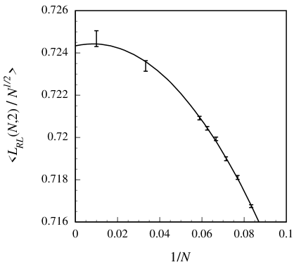
Figure 2: Finite size scaling of mean optimum tour length for $d=2$. Best fit ($\chi^{2}=4.46$) is given by: $\langle L_{RL}(N,2)\rangle/N^{1/2}=0.7243(1+0.0322/N-1.886/N^{2})$. Error bars show one standard deviation (statistical error).

Let us now consider the large $N$ limit of $L_{RL}(N,2)/\sqrt{N}$, as given by numerical simulations. In the Euclidean case, it has been observed [7] that the finite size scaling law can be written in terms of a power series in $1/N$. The same arguments given there apply to the random link case, and so we may expect the ensemble average $\langle L_{RL}(N,2)\rangle$ to satisfy

$$\langle L_{RL}(N,d)\rangle=\beta_{RL}(d)\,N^{1-1/d}\,\left[1+\frac{A(d)}{N}+\cdots\right]\mbox{.}$$ (16)

In order to obtain $\langle L_{RL}(N,2)\rangle$ at a finite value of $N$ from simulations, we average over a large number of instances to reduce the statistical error arising from instance-to-instance fluctuations. Figure 2 shows the results of this, with accompanying error bars, fitted to the expected finite size scaling law (truncated after $O(1/N^{2})$). The fit is a good one: $\chi^{2}=4.46$ for 5 degrees of freedom. As in [7], we may obtain an error estimate on $\beta_{RL}(2)$ by noting that if we take the extrapolated value and add or subtract one standard deviation, and then redo the fit with this as a fixed constant, $\chi^{2}$ will increase by 1. We thus find $\beta_{RL}(2)=0.7243\pm 0.0004$, in very good agreement with the cavity result of $\beta_{RL}^{c}(2)=0.7251\ldots$ The discrepancy between the two is consistent with the statistical error (two standard deviations apart), and in relative terms is approximately $0.1\%$. The fit in Figure 2, furthermore, appears robust with respect to sub-samples of the data; even if we disallow the use of the $N=100$ data point in the fit, the resulting asymptotic value is still within $0.25\%$ of the cavity prediction. By comparison, recall that the error in the replica symmetric solution to the SK spin glass ground state energy is of the order of $5\%$ [5].

Figure 3: Integrated probability distribution of link lengths in the optimal tour, for $d=2$, using rescaled length $\tilde{l}=l\sqrt{N}$. Plus signs represent $N=12$ simulation results, dots represent $N=100$ simulation results, and solid line represents cavity prediction.

Another quantity that Krauth and Mézard studied in their $d=1$ numerical investigation [4] was the optimum tour link length distribution ${\cal P}_{d}(l)$ given in (11). Let us consider ${\cal P}_{2}(l)$, and following their example, let us look specifically at the integrated distribution $I_{d}(l)\equiv\int_{0}^{l}{\cal P}_{d}(l^{\prime})\,dl^{\prime}$. The cavity result for $I_{d}(l)$ can, like $\beta_{RL}(d)$, be computed numerically to arbitrary precision. In Figure 3 we compare this with the results of direct simulations, for $d=2$, at increasing values of $N$. The improving agreement for increasing $N$ (within 2% at $N=100$) strongly suggests that the cavity solution gives the exact $N\to\infty$ result.

Figure 4: Frequencies with which $k$th-nearest neighbors are used in optimal 2-D random link tours. Plus signs show values for $N=12$, squares for $N=17$, diamonds for $N=30$, and dots for $N=100$. Best exponential fit (straight line on log plot) is shown for $N=100$ data.

Finally, it is of interest to consider one further quantity in the $d=2$ random link simulations, for which there is at present no corresponding cavity prediction: the frequencies of “neighborhood rank” used in the optimal tour, that is, the proportion of links connecting nearest neighbors, 2nd-nearest neighbors, etc. Sourlas [6] has noted that in practice in the $d=1$ case, this frequency falls off rapidly with increasing neighborhood rank — suggesting that optimization heuristics could be improved by preferentially choosing links between very near neighbors. Our simulations show (see Figure 4) that for $d=2$ the decrease is astonishingly close to exponential. We may offer the following qualitative explanation for this behavior. An optimal tour will always try to use links to the closest neighbors possible. While the constraint of a closed loop may force it in rare cases to use neighbors of high rank, this will apply only to a very small number of links in the tour. Connecting a point to, say, its $k$th-nearest neighbor will for the most part be profitable only when this neighbor is not much further away than the $k-1$ nearer neighbors. In other words, the lengths from the point to its $k$ closest neighbors would have to be nearly degenerate. Since a $k$-fold degeneracy of this sort is the product of $k-1$ unlikely events, it is in fact quite natural that the probability of such an occurrence is exponentially small in $k$.

We therefore conjecture that the neighborhood frequency function will fall exponentially in $k$ at large $k$. We expect this behavior to hold in any dimension, and for that matter, in the Euclidean TSP as well. Similar and even stronger numerical results have been reported [21] in another link-based combinatorial optimization problem, the matching problem. An analytical calculation of the neighborhood frequency may indeed turn out to be feasible using the cavity approach, thus providing a theoretical prediction to accompany our conjecture. We consider this a significant open question.

4 Numerical analysis: renormalized model

In this section we will consider a different sort of random link TSP, proposed in [7], allowing us to test numerically the $1/d$ coefficient predicted by the cavity result (14). The approach involves introducing a mapping that shifts and rescales all the lengths between cities. By taking the limit $d\to\infty$, one obtains a $d$-independent random link model having an exponential distribution for its link lengths. This “renormalized” model was outlined in [7]; we present it here in further detail. We then perform a numerical study of the model, which enables us to determine the large $d$ behavior of the standard $d$-dimensional random link model.

Let us define $\langle D_{1}(N,d)\rangle$ to be the distance between a city and its nearest neighbor, averaged over all cities in the instance and over all instances in the ensemble. For large $d$, it may be shown [7] that

$$\lim_{N\to\infty}N^{1/d}\langle D_{1}(N,d)\rangle=\sqrt{\frac{d}{2\pi e}}\,(\pi d)^{1/2d}\left[1-\frac{\gamma}{d}+O\left(\frac{1}{d^{2}}\right)\right]$$ (17)

where $\gamma$ is Euler’s constant. It is not surprising that this quantity is reminiscent of (15), since $N^{1/d}\langle D_{1}(N,d)\rangle$ represents precisely a lower bound on $\beta_{RL}(d)$.

In order to obtain the renormalized model, consider a link length transformation making use of $\langle D_{1}(N,d)\rangle$. For any instance with link lengths $l_{ij}$ (taken to have the usual distribution (10) corresponding to $d$ dimensions), define new link lengths $x_{ij}\equiv d[l_{ij}-\langle D_{1}(N,d)\rangle]/\langle D_{1}(N,d)\rangle$. The $x_{ij}$ are “lengths” only in the loosest sense, as they can be both positive and negative. The optimal tour in the $x_{ij}$ model will, however, follow the same “path” as the optimal tour in the associated $l_{ij}$ model, since the transformation is linear. Its length $L_{x}(N,d)$ will simply be given in terms of $L_{RL}(N,d)$ by:

$$L_{x}(N,d) = d\,\frac{L_{RL}(N,d)-N\langle D_{1}(N,d)\rangle}{\langle D_{1}(N,d)\rangle}\mbox{, so}$$ (18)

$$L_{RL}(N,d) = N\langle D_{1}(N,d)\rangle\,\left[1+\frac{L_{x}(N,d)}{dN}\right]\mbox{.}$$ (19)

In the standard $d$-dimensional random link model, $\beta_{RL}(d)=\lim_{N\to\infty}L_{RL}(N,d)/N^{1-1/d}$, so

$$\beta_{RL}(d) = \lim_{N\to\infty}N^{1/d}\langle D_{1}(N,d)\rangle\,\left[1+\frac{L_{x}(N,d)}{dN}\right]\mbox{, and at large $d$, using (\ref{eq_d1}),}$$ (20)

$$= \sqrt{\frac{d}{2\pi e}}\,(\pi d)^{1/2d}\left[1-\frac{\gamma}{d}+O\left(\frac{1}{d^{2}}\right)\right]\,\lim_{N\to\infty}\left[1+\frac{L_{x}(N,d)}{dN}\right]\mbox{.}$$

As $\beta_{RL}(d)$ is a well-defined quantity, there must exist a value $\mu(d)$ such that $\lim_{N\to\infty}L_{x}(N,d)/N=\mu(d)$.

Now, what will be the distribution of “renormalized lengths” $\rho(x)$ corresponding to $\rho(l)$? From (10) and the definition of the $x_{ij}$,

$$\rho(x) = \frac{d\,\pi^{d/2}\,l^{d-1}}{\Gamma(d/2+1)}\,\frac{\langle D_{1}(N,d)\rangle}{d}\mbox{, and substituting for $l$,}$$ (21)

$$= \frac{\pi^{d/2}}{\Gamma(d/2+1)}\,\left(1+\frac{x}{d}\right)^{d-1}\,\langle D_{1}(N,d)\rangle^{d}\mbox{.}$$

In the limit $N\to\infty$, we thus obtain from (17) the large $d$ expression:

$$\rho(x) \sim \frac{\pi^{d/2}}{\Gamma(d/2+1)}\,\left(1+\frac{x}{d}\right)^{d-1}N^{-1}\,\left(\frac{d}{2\pi e}\right)^{d/2}\sqrt{\pi d}\,\left[1-\frac{\gamma}{d}+\cdots\right]^{d}$$ (22)

$$\sim N^{-1}\left(1-\frac{\gamma}{d}\right)^{d}\left(1+\frac{x}{d}\right)^{d-1}\left[1+O\left(\frac{1}{d}\right)\right]\mbox{ by Stirling's formula}$$

$$\sim N^{-1}e^{x-\gamma}\,\left[1+O\left(\frac{1}{d}\right)\right].$$

In the limit $d\to\infty$, $\rho(x)$ will be independent of $d$; the same must then be true for $L_{x}(N,d)$, and consequently for $\mu(d)$.

Let us now define the renormalized model as being made up of link “lengths” $x_{ij}$ in this limit. This results in a somewhat peculiar random link TSP, no longer containing the parameter $d$. Its link length distribution is given by the $d\to\infty$ limit of (22),

$$\rho(x)=N^{-1}\exp(x-\gamma),$$ (23)

and its optimum tour length satisfies

$$\lim_{N\to\infty}\frac{L_{x}(N)}{N}=\mu,$$ (24)

where we have dropped the $d$ argument from these (now $d$-independent) quantities. By performing direct simulations using the distribution (23) — cut off beyond a threshold value of $x$, as was done for $\rho_{d}(l)$ — we may find the value of $\mu$ numerically.

Figure 5: Distribution of renormalized random link rescaled tour length $(L_{x}-\langle L_{x}\rangle)/N$ for increasing values of N. Plus signs show $N=12$ (100,000 instances used), squares show $N=17$ (100,000 instances used), diamonds show $N=30$ (4,000 instances used), and dots show $N=100$ (1,200 instances used). Solid lines represent Gaussian fits for each value of $N$ plotted.

Finally, let us relate this renormalized model to the standard $d$-dimensional random link model. In light of (24), we may rewrite (20) and obtain the result given in [7]:

$$\beta_{RL}(d)=\sqrt{\frac{d}{2\pi e}}\,(\pi d)^{1/2d}\left[1+\frac{\mu-\gamma}{d}+O\left(\frac{1}{d^{2}}\right)\right]\mbox{.}$$ (25)

The value of $\mu$ in the renormalized model therefore gives directly the $1/d$ coefficient for the (non-renormalized) $\beta_{RL}(d)$.

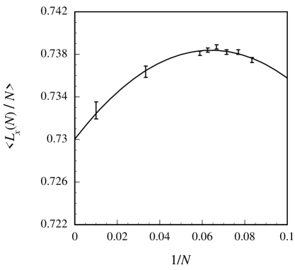
Figure 6: Finite size scaling of renormalized model optimum. Best fit ($\chi^{2}=5.23$) is given by: $\langle L_{x}(N)\rangle/N=0.7300(1+0.3575/N-2.791/N^{2})$. Error bars show one standard deviation (statistical error).

We now carry out these direct simulations for the renormalized model. Figures 5 and 6 show our numerical results. In Figure 5, we see that just as in the $d=2$ case, the distribution of the optimum tour length becomes sharply peaked at large $N$ and the asymptotic limit $\mu$ is well-defined. Via (25), this provides very good reason for believing that $\beta_{RL}(d)$ is well-defined for all $d$, and that self-averaging holds for the random link TSP in general. In Figure 6, we show the finite size scaling of $\langle L_{x}(N)/N\rangle$. The fit is again quite satisfactory (with $\chi^{2}$=5.23 for 5 degrees of freedom), giving the asymptotic result $\mu=0.7300\pm 0.0010$. The resulting value for the $1/d$ coefficient in $\beta_{RL}(d)$ is then $\mu-\gamma=0.1528\pm 0.0010$, in excellent agreement (error under $0.3\%$) with the cavity prediction $2-\ln 2-2\gamma=0.1524\ldots$ given in (14).

Figure 7: Frequencies with which $k$th-nearest neighbors are used in optimal renormalized random link tours. Plus signs show values for $N=12$, squares for $N=17$, diamonds for $N=30$, and dots for $N=100$. Best exponential fit (straight line on log plot) is shown for $N=100$ data.

Again, as in the $d=2$ case, let us briefly consider the frequencies of $k$th-nearest neighbors used in optimal tours. These frequencies are given in Figure 7 for the renormalized model. Even though the exponential fit is not as good as in the $d=2$ case, it is still striking here. What does this tell us, in turn, about the standard random link TSP? Recall that the renormalized model arises from the $d\to\infty$ limit of the $d$-dimensional (non-renormalized) model, and that the mapping (18) preserves the optimum tour for any given instance. These $k$th-neighbor frequency results are thus the $d\to\infty$ limiting frequencies for the $d$-dimensional random link TSP (and most likely for the Euclidean TSP also). This gives further support to our conjecture that the exponential law holds for all $d$, and suggests as a consequence that the “typical” neighborhood rank $k$ used in optimal tours remains bounded for all $d$.

5 Conclusion

The random link TSP has interested theoreticians primarily because of its analytical tractability, allowing presumably exact results that are not possible in the more traditional Euclidean TSP. Other than in the $d=1$ case, however, it has attracted little attention. In this paper we have provided a numerical study of the random link TSP that was lacking up to this point, addressing important unanswered questions. Through simulations, we have tested the validity of the theoretical predictions derived using the cavity method. While in other disordered systems, such as spin glasses, the replica symmetric solution gives values of macroscopic quantities that are inexact (typically by several percent), in the random link TSP it shows all signs of being exact. We have studied various link-based quantities at $d=2$ and found that the numerical results confirm the cavity predictions to within $0.1\%$. Furthermore, we have confirmed, by way of simulations on a renormalized random link model, that the analytical cavity solution gives a large $d$ expansion for the optimum tour length whose $1/d$ coefficient is correct to within well under $1\%$. The excellent agreement found at $d=1$ [4, 6], $d=2$, and to $O(1/d)$ at large $d$, then suggest strongly that the cavity predictions are exact. This provides indirect evidence that the assumption of replica symmetry — on which the cavity calculation is based — is indeed justified for the TSP.

Finally, our random link simulations have pointed to a surprising numerical result. If one considers the links in optimal tours as links between $k$th-nearest neighbors, at $d=2$ the frequency with which the tour uses neighborhoods of rank $k$ decreases with $k$ as almost a perfect exponential. Encouraged by similar results in the renormalized model, we conjecture that this property holds true for all $d$, as well as in the Euclidean TSP. As no theoretical calculation presently explains the phenomenon, we would welcome further investigation along these lines.

References

- [1] S. Kirkpatrick and G. Toulouse, Configuration space analysis of travelling salesman problem, J. Phys. France 46:1277–1292 (1985).
- [2] D. Sherrington and S. Kirkpatrick, Solvable model of a spin-glass, Phys. Rev. Lett. 35:1792–1796 (1975).
- [3] M. Mézard and G. Parisi, Mean-field equations for the matching and the travelling salesman problems, Europhys. Lett. 2:913–918 (1986).
- [4] W. Krauth and M. Mézard, The cavity method and the travelling-salesman problem, Europhys. Lett. 8:213–218 (1989).
- [5] M. Mézard, G. Parisi and M. A. Virasoro (eds.), Spin Glass Theory and Beyond (World Scientific, Singapore, 1987).
- [6] N. Sourlas, Statistical mechanics and the travelling salesman problem, Europhys. Lett. 2:919–923 (1986).
- [7] N. J. Cerf, J. Boutet de Monvel, O. Bohigas, O. C. Martin and A. G. Percus, The random link approximation for the Euclidean traveling salesman problem, J. Phys. I France 7:117–136 (1997).
- [8] M. Mézard and G. Parisi, A replica analysis of the travelling salesman problem, J. Phys. France 47:1285–1296 (1986).
- [9] P. G. De Gennes, Exponents for the excluded volume problem as derived by the wilson method, Phys. Lett. A 38:339–340 (1972).
- [10] H. Orland, Mean-field theory for optimization problems, J. Phys. Lett. France 46:L763–L770 (1985).
- [11] A. G. Percus, Voyageur de commerce et problèmes stochastiques associés, Ph.D. thesis, Université Pierre et Marie Curie, Paris (1997).
- [12] D. S. Johnson, L. A. McGeoch and E. E. Rothberg, Asymptotic Experimental Analysis for the Held-Karp Traveling Salesman Bound, 7th Annual ACM-SIAM Symposium on Discrete Algorithms (Atlanta, 1996), pp. 341–350.
- [13] A. G. Percus and O. C. Martin, Finite size and dimensional dependence in the Euclidean traveling salesman problem, Phys. Rev. Lett. 76:1188–1191 (1996).
- [14] J. H. Boutet de Monvel, Physique statistique et modèles à liens aléatoires, Ph.D. thesis, Université Paris-Sud (1996).
- [15] R. Brunetti, W. Krauth, M. Mézard and G. Parisi, Extensive numerical solutions of weighted matchings: Total length and distribution of links in the optimal solution, Europhys. Lett. 14:295–301 (1991).
- [16] J. Beardwood, J. H. Halton and J. M. Hammersley, The shortest path through many points, Proc. Cambridge Philos. Soc. 55:299–327 (1959).
- [17] J. Vannimenus and M. Mézard, On the statistical mechanics of optimization problems of the travelling salesman type, J. Phys. Lett. France 45:L1145–L1153 (1984).
- [18] S. Lin and B. Kernighan, An effective heuristic algorithm for the traveling salesman problem, Operations Res. 21:498–516 (1973).
- [19] O. C. Martin and S. W. Otto, Combining simulated annealing with local search heuristics, Ann. Operations Res. 63:57–75 (1996).
- [20] M. Mézard, G. Parisi, N. Sourlas, G. Toulouse and M. Virasoro, Replica symmetry breaking and the nature of the spin glass phase, J. Phys. France 45:843–854 (1984).
- [21] J. Houdayer, J. H. Boutet de Monvel and O. C. Martin, Comparing mean field and Euclidean matching problems, Eur. Phys. J. B, in press.