Calculation of the Phase Behavior of Lipids

Abstract

The self-assembly of monoacyl lipids in solution is studied employing a model in which the lipid’s hydrocarbon tail is described within the Rotational Isomeric State framework and is attached to a simple hydrophilic head. Mean-field theory is employed, and the necessary partition function of a single lipid is obtained via a partial enumeration over a large sample of molecular conformations. The influence of the lipid architecture on the transition between the lamellar and inverted-hexagonal phases is calculated, and qualitative agreement with experiment is found.

1 Introduction

Lipid bilayers form the framework of biological membranes. Nevertheless almost all membrane lipids adopt non-bilayer configurations, either in their pure state or in lipid mixtures, under conditions close to physiological ones [1, 2]. Although cubic phases are also found [1, 3], the most commonly occurring non-bilayer arrangement is the inverted-hexagonal[4], or $H_{II}$, phase in which a matrix of hydrocarbon tails is pierced by a hexagonal array of water-filled tubes lined by the hydrophilic head groups. Why biological membranes should contain lipids which tend to drive it towards a configurational instability, much like a lamellar-hexagonal transition, has been the subject of much speculation centering on the role such instabilities might play in promoting membrane fusion, and controlling membrane permeability[2, 5]. As a consequence of this interest, there have been many studies of the phase behavior of lipids in general, and of the parameters which affect the lamellar to hexagonal transition in particular[6, 7, 8, 9, 10]. For example, in a homologous series of saturated diacyl or diakyl phosphatidylethanolamines, an increase of chain length stabilizes the $H_{II}$ phase, causing the transition temperature between it and the lamellar phase, which exists at lower temperatures, to decrease[6]. Conversely an increase in the volume of the head group stabilizes the lamellar phase, $L_{\alpha}$, causing the transition temperature to increase, as clearly demonstrated[8] in mixtures of dioleoylphosphatidylethanolamine, DOPE, and dioleoylphosphatidylcholine, DOPC. An increase in water content also tends to stabilize $H_{II}$.

A qualitative understanding of these results is provided by a characterization of the lipid as a simple geometrical object parameterized by the chain volume, the maximum chain length, and the head-group area [11]. The different phases result from simple geometrical packing considerations. In contrast to simplifying the description of the lipid, large-length scale approaches[8, 12] simplify the description of the bilayer itself, reducing it to an infinitesimally thin membrane characterized by elastic constants which are inputs to the theories[13]. Often, elements of such theories are combined with other phenomenological terms to complete the description[8].

Simulation of chemically realistic models of lipids and their interactions have been carried out[14], and yield valuable information about local properties, such as density and orientation profiles in the bilayer, lamellar phase, and dynamic and transport properties. However simulations are both demanding computationally and limited to a rather small number of particles. Within the framework of chemically realistic models, the simulation of phase transitions between different morphologies seems not to be feasible at present.

Analytic, mean-field, approaches combined with microscopic modeling of the tails of lipids, have been applied with success to the manner in which the tails pack in the interior of aggregates [15, 16, 17]. The contribution of the chains to the single-lipid partition function, required by mean-field theory, is obtained from an enumeration of the molecular conformations of the tails permitted within the Rotational Isomeric State (RIS) model[18]. It is here that the particular architecture of the chains enters. Bilayer thickness is set by assumptions on a phenomenological free-energy describing the head-group region. These calculations reproduce many features of the density profiles and segment orientations in the interior of aggregates.

The contribution of the lipid tails to the $H_{II}$ phase has also been examined by these means[19], and it was shown that their entropy always favors this phase over the lamellar one. It was also observed that a change in the area per head group could lead to a transition to the lamellar phase. No solvent was included explicitly, but as its effect would be to alter the area per head group, the observation indicates that variation of solvent concentration would be able to bring about a transition. The calculation is an approximate one by necessity because it is carried out in real space. The full $p6mm$ symmetry of the $H_{II}$ phase is not preserved, as the tubes are considered to be cylinders on which the area per head group is uniform. Further, the packing constraints in the interstices between the tubes cannot be satisfied exactly. Application of this real-space approach to such complicated morphologies as $Ia\bar{3}d$ would be extremely laborious[20].

In this paper, we overcome the difficulties of a real-space approach by combining the above enumeration techniques with recent advances in the solution of mean-field equations of polymers [21, 22], a combination which we had previously shown to be fruitful in a relatively simple system[23]. Here we apply it to a more complicated system, a minimal model of a lipid and solvent mixture, one which treats the head group on the same microscopic basis as the tails. We are able, thereby, to obtain its phase diagram within mean-field theory and to examine how the boundary between $L_{\alpha}$ and $H_{II}$ phases changes with lipid architecture, i.e. how that architecture affects the stability of the lamellar phase. Our results are in qualitative agreement with experiment.

2 Model and numerical Self-Consistent Field technique

We describe the lipid as consisting of a tail, comprised of any number of chains, (usually two), containing altogether a total of $N$ identical segments of volume $v_{t}$ each, and a head containing two segments of volume $v_{h}/2$ each. The solvent molecules have volume $v_{s}$ but are otherwise without structure. The partition function of the mixture of $N_{L}$ lipid molecules and $N_{S}$ solvent particles in volume $V$ can be written

$${\cal Z}\sim\frac{1}{N_{S}!N_{L}!}\int\prod_{\alpha=1}^{N_{L}}{\cal D}{\bf r}_{\alpha}P[{\bf r}_{\alpha}]\;\;\;\prod_{\beta=1}^{N_{S}}d{\bf r}_{\beta}\delta\left(1-\hat{\Phi}_{s}-\frac{v_{h}}{v_{s}}\hat{\Phi}_{h}-\frac{v_{t}}{v_{s}}\hat{\Phi}_{t}\right)\exp\left\{\frac{-{\cal E}}{k_{B}T}\right\}$$ (1)

where

$$\hat{\Phi}_{h}=v_{s}\sum_{\alpha=1}^{N_{L}}\frac{1}{2}\sum_{h=1}^{2}\delta({\bf r}-{\bf r}_{\alpha,h}),$$ (2)

$$\hat{\Phi}_{t}=v_{s}\sum_{\alpha=1}^{N_{L}}\sum_{t=1}^{N}\delta({\bf r}-{\bf r}_{\alpha,t}),$$ (3)

are the dimensionless number densities of the head and the tail segments, and

$$\hat{\Phi}_{s}=v_{s}\sum_{\alpha=1}^{N_{S}}\delta({\bf r}-{\bf r}_{\alpha,s}),$$ (4)

is the dimensionless number density of solvent particles. The fluid has been treated as incompressible. The probability distribution of the lipid configurations is denoted $P[{\bf r}_{\alpha}]$, and the interaction energy between particles is ${\cal E}$.

It is convenient to introduce auxiliary fields and consider the particles to interact with one another via intermediate, fluctuating fields rather than directly;

$${\cal Z}\sim\int{\cal D}\Phi_{h}{\cal D}\Phi_{t}{\cal D}\Phi_{s}{\cal D}W_{h}{\cal D}W_{t}{\cal D}W_{s}{\cal D}\Pi\exp\left\{-\frac{{\cal F}}{k_{B}T}\right\}$$ (5)

where the free energy functional, ${\cal F}$, is

$$\frac{{\cal F}[\Phi_{h},\Phi_{t},\Phi_{s},W_{h},W_{t},W_{s},\Pi]}{k_{B}T} = \frac{{\cal E}}{k_{B}T}-N_{S}\ln\frac{{\cal Q}_{S}}{N_{S}}-N_{L}\ln\frac{{\cal Q}_{L}}{N_{L}}$$

$$-\frac{1}{v_{s}}\int d{\bf r}\;{\Big{\{}}W_{h}\Phi_{h}+W_{t}\Phi_{t}+W_{s}\Phi_{s} +\Pi\left(1-\Phi_{s}-\frac{v_{h}}{v_{s}}\Phi_{h}-\frac{v_{t}}{v_{s}}\Phi_{t}\right){\Big{\}}}$$ (6)

In this expression, ${\cal Q}_{L}$ denotes the single lipid partition function in the external fields $W_{h}$ and $W_{t}$, acting on head and tail segments, and ${\cal Q}_{S}$ the solvent partition function;

$${\cal Q}_{L}[W_{h},W_{t}]=\int{\cal D}{\bf r}P[{\bf r}]\exp\left\{-\frac{1}{2}\sum_{h=1}^{2}W_{h}({\bf r}_{h})-\sum_{t=1}^{N}W_{t}({\bf r}_{t})\right\},$$ (7)

$${\cal Q}_{S}[W_{s}]=\int d{\bf r}\;\exp{\Big{\{}}-W_{s}({\bf r}){\Big{\}}}$$ (8)

The interaction energy is

$$\frac{{\cal E}}{k_{B}T}=\frac{1}{2}\int\frac{d{\bf r}}{v_{s}}\frac{d{\bf r}^{\prime}}{v_{s}}\sum_{\alpha,\beta}V_{\alpha\beta}({\bf r}-{\bf r}^{\prime})\Phi_{\alpha}({\bf r})\Phi_{\beta}({\bf r}^{\prime}),$$ (9)

where $\alpha$ and $\beta$ take the values $h$, $t$, and $s$. The incompressibility condition

$$\Phi_{s}({\bf r})+\frac{v_{h}}{v_{s}}\Phi_{h}({\bf r})+\frac{v_{t}}{v_{s}}\Phi_{t}({\bf r})=1,$$ (10)

can be used to eliminate the solvent volume fraction $\Phi_{s}$ in Eq.(9). The terms linear in the head and tail volume fractions which result from this procedure can be ignored, as they only contribute to the chemical potentials of the heads and tails. At this stage we neglect the coupling between the molecular conformations, the local fluid-like packing of molecular segments, and the local energy density and assume that all interactions are contact interactions,

$$V_{\alpha\beta}({\bf r}-{\bf r}^{\prime})=\epsilon_{\alpha\beta}\delta({\bf r}-{\bf r}^{\prime}).$$ (11)

With these simplifications, the energy can be written in the form

$$\frac{{\cal E}[\Phi_{h},\Phi_{t}]}{k_{B}T}=\frac{1}{v_{s}}\int d{\bf r}\;\left\{\chi_{ht}\Phi_{h}\Phi_{t}-\frac{1}{2}\chi_{hh}\Phi_{h}^{2}-\frac{1}{2}\chi_{tt}\Phi_{t}^{2}\right\},$$ (12)

with

$$\chi_{ht} \equiv \frac{1}{v_{s}k_{B}T}\left[\epsilon_{ht}+\epsilon_{ss}\frac{v_{h}v_{t}}{v_{s}^{2}}-\epsilon_{hs}\frac{v_{t}}{v_{s}}-\epsilon_{ts}\frac{v_{h}}{v_{s}}\right]$$ (13)

$$\chi_{hh} \equiv -\frac{1}{v_{s}k_{B}T}\left[\epsilon_{hh}+\epsilon_{ss}\frac{v_{h}^{2}}{v_{s}^{2}}-2\epsilon_{hs}\frac{v_{h}}{v_{s}}\right]$$ (14)

$$\chi_{tt} \equiv -\frac{1}{v_{s}k_{B}T}\left[\epsilon_{tt}+\epsilon_{ss}\frac{v_{t}^{2}}{v_{S}^{2}}-2\epsilon_{ts}\frac{v_{h}}{v_{s}}\right].$$ (15)

The functional integration in Eq. (5) cannot be carried out explicitly. Therefore we employ mean-field theory, which approximates the integral by the largest value of the integrand. This maximum occurs at values of the fields and densities which are determined by extremizing ${\cal F}$ with respect to each of its seven arguments. Fluctuations around these most probable values are neglected. These values are denoted below by lower case letters. They satisfy the self-consistent equations

$$w_{h}({\bf r}) = \chi_{ht}\phi_{t}({\bf r})-\chi_{hh}\phi_{h}({\bf r})+\pi({\bf r})v_{h}/v_{s},$$ (16)

$$w_{t}({\bf r}) = \chi_{ht}\phi_{h}({\bf r})-\chi_{tt}\phi_{t}({\bf r})+\pi({\bf r})v_{t}/v_{s},$$ (17)

$$w_{s}({\bf r}) = \pi({\bf r}),$$ (18)

$$1 = \phi_{s}({\bf r})+\phi_{h}({\bf r})v_{h}/v_{s}+\phi_{t}({\bf r})v_{t}/v_{s},$$ (19)

$$\phi_{h}({\bf r}) = -\frac{N_{L}v_{s}}{{\cal Q}_{L}}\frac{\delta{\cal Q}_{L}}{\delta w_{h}({\bf r})},$$ (20)

$$\phi_{t}({\bf r}) = -\frac{N_{L}v_{s}}{{\cal Q}_{L}}\frac{\delta{\cal Q}_{L}}{\delta w_{t}({\bf r})},$$ (21)

$$\phi_{s}({\bf r}) = -\frac{N_{S}v_{s}}{{\cal Q}_{S}}\frac{\delta{\cal Q}_{S}}{\delta w_{s}({\bf r})}.$$ (22)

Because the overall density is fixed, we can set $\int d{\bf r}\pi({\bf r})$ $=\int d{\bf r}w_{s}({\bf r})=0$. The mean-field free energy $F\equiv{\cal F}[\phi_{h},\phi_{y},\phi_{s},w_{h},w_{t},w_{s},\pi]$ is

$$\frac{v_{s}F}{Vk_{B}T}=\phi_{s}\ln\phi_{s}+\phi_{L}\ln\phi_{L}-\phi_{s}\ln\frac{{\cal Q}_{S}v_{s}}{V}-\phi_{L}\ln\frac{{\cal Q}_{L}v_{s}}{V}$$

$$+\frac{1}{V}\int d{\bf r}\;\left\{-\chi_{ht}\phi_{h}({\bf r})\phi_{t}({\bf r})+\frac{1}{2}\chi_{hh}\phi_{h}^{2}({\bf r})+\frac{1}{2}\chi_{tt}\phi_{t}^{2}({\bf r})\right\},$$ (23)

where we have denoted $\phi_{s}\equiv N_{s}v_{s}/V$, the average, dimensionless, number density of solvent, and similarly $\phi_{L}\equiv N_{L}v_{s}/V$, for lipids.

In order to study the self-assembly of lipids into various morphologies, we expand the spatial dependence of the densities and fields in a complete set of orthonormal functions $\{f_{k}({\bf r})\}$, $V^{-1}\int d{\bf r}\;f_{i}f_{k}=\delta_{ik},\;f_{1}=1$, which possess the symmetry of the morphology being considered[21]; e.g. $\phi_{h}({\bf r})=\sum_{k}\phi_{h,k}f_{k}({\bf r})$. The coefficients $\phi_{h,1}$, $\phi_{t,1}$, and $\phi_{s,1}$ are simply equal to the average, dimensionless number densities $\phi_{h}$, $\phi_{t}$, and $\phi_{s}$ respectively. The solvent density $\phi_{s}({\bf r})=\phi_{s,1}V\exp[-w_{s}({\bf r})]/\int d{\bf r}\;\exp[-w_{s}]({\bf r})$ can be Fourier expanded as $\phi_{s,k}=\phi_{s,1}(\exp S)_{k,1}/(\exp S)_{1,1},$ with

$$\qquad(S)_{k,m}=-\sum_{n}w_{s,n}\frac{1}{V}\int d{\bf r}\;f_{k}f_{n}f_{m}.$$ (24)

The partition function of a single lipid in an external field cannot be obtained analytically for a realistic architecture. Therefore we approximate the non-interacting single lipid probability distribution ${\cal P}$ by a representative sample of ${\cal N}$ single lipid conformations. Assigning the Boltzmann weight, $\omega_{c}$, to each lipid conformation in the field of mean potentials $w_{h}$ and $w_{t}$

$$\omega_{c}\equiv\exp\left\{-\sum_{k}\left(w_{h,k}\frac{1}{2}\sum_{h=1}^{2}f_{k}({\bf r}_{c,h})+w_{t,k}\sum_{t=1}^{N}f_{k}({\bf r}_{c,t})\right)\right\}$$ (25)

we obtain from Eq. (21) the components of the tail segment density

$$\phi_{t,k}=\phi_{t,1}\frac{\sum_{c=1}^{\cal N}\omega_{c}\sum_{t=1}^{N}f_{k}({\bf r}_{c,t})}{\sum_{c=1}^{\cal N}\omega_{c}},$$ (26)

and similarly for the head segment density. The self-consistent equations, expressed in the basis $\{f_{k}\}$, are solved by a Newton-Raphson-like method. Finally we minimize the free energy with respect to the size of the unit cell, $D$. To this end we translate the lipid conformations so as to achieve a uniform distribution in the cell.

3 Results

The above scheme is applicable to arbitrary lipid architecture and symmetry of spatial ordering. We have applied it to model monoolein, a fatty acid whose phase behavior in water has attracted much interest[10, 24]. A schematic sketch of the architecture is presented in Fig. 1 to illustrate the architectural parameters of our model. The single hydrocarbon tail contains $N=17$ units, a distance $\ell=1.53$Å apart, with a double bond between the 8th and 9th units. The volume of the tail units is $v_{t}=29$ ų. The trans-gauche energy difference is taken to be 500cal/mole. We take the two units of the head and the first segment of the tail to be collinear, with a distance $d$ between the head units, and a distance $b$ between the first tail segment and the adjacent head unit. We set all interactions to zero save those between hydrophilic and hydrophobic entities, and they are taken to have the same strength $\epsilon$. Thus from Eqs. (13-15), $\chi_{hh}=0$, $\chi_{tt}=(2\epsilon v_{t}/k_{B}Tv_{s}^{2})\equiv\chi$, and $\chi_{ht}=\chi(v_{s}-v_{h})/(2v_{t})$. Typically between 524,288 and 2,097,152 conformations of single lipids were generated. The position of the head was chosen uniformly distributed over the unit cell, with a random orientation. The tail was then constructed according to the Rotational Isomeric State (RIS) model[18]. The tail conformations were generated at a temperature of 300K, so that they are fluid.

We use up to 32 basis functions, $f_{k}({\bf r})$. Because the calculations involve the contributions of each individual lipid to the Fourier component of the density, the required computer memory scales like the product of lipid conformations and number of basis functions. The program needs more than 1 Gbyte memory. We employ a massively parallel computer CRAY T3D/T3E and distribute the lipid conformations among the processors independently of their spatial position. Each processor evaluates the contribution of its assigned lipid conformations to the Fourier components of the density according to eqn. (26). The partial results are collected via shmem routines. The first processor also calculates the solvent density, and therefore we assign it a smaller number of lipid conformations to compensate for the additional work load. Typically between 32 and 128 processors have been employed in parallel. The program scales linearly with the number of processors.

We first consider the parameters $v_{t}/v_{s}=1$, $v_{h}/v_{s}=3.2$, $d/\ell=0$, and $b/\ell=1$. Thus the head is a relatively small, single, interaction center located the same distance from the first tail segment as each tail segment is from its neighbors on the chain. The ratio of solvent volume, $v_{s}$, to lipid volume, $v_{l}=v_{h}+Nv_{t}$, determines the extent to which the microstructure can be swollen. Small solvents tend to swell the microstructure due to their large translational entropy, whereas large solvents favor phase separation. The phase diagram is determined by calculating the free energy of the different morphologies as a function of the solvent concentration and the “temperature” $1/\chi$. Phase coexistence is determined by equating the chemical potential

$$\mu=\frac{\partial F}{\partial N_{s}}=\frac{v_{s}\partial F}{V\partial\phi_{s}},$$ (27)

and the Gibbs free energy

$$\frac{G}{V}=\frac{F}{V}-\frac{\mu\phi_{s}}{v_{s}},$$ (28)

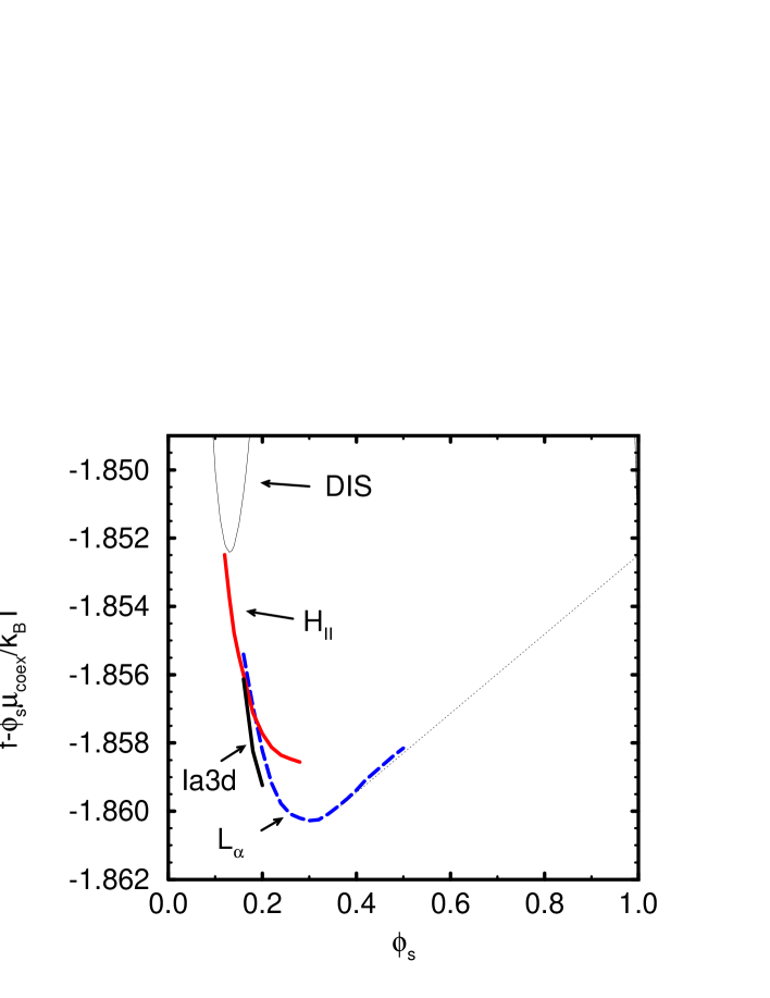
Figure 2: Free energies at $1/\chi_{tt}=0.25$ of the disordered, $L_{\alpha}$, $Ia\bar{3}d$, and $H_{II}$ phases as function of the solvent content. For convenience, the term $\mu_{coex}\phi_{s}/k_{B}T$ has been subtracted from the dimensionless free-energy density $f$, where $\mu_{coex}$ is the chemical potential at which solvent-rich and solvent-poor disordered phases would coexist were there no stable ordered phases. The dotted line shows the Maxwell construction between the $L_{\alpha}$ and the solvent-rich disordered phase.

in the two phases. For a representative value of the temperature, $1/\chi=0.25$, we find the sequence of dimensionless free energy densities, $f\equiv v_{s}F/Vk_{B}T$, shown in Fig. 2. It follows from this sequence that, with increasing solvent concentration, there is a transition from the disordered phase to the $H_{II}$ phase, and from that to the $Ia\bar{3}d$ cubic phase. At larger concentrations, the lamellar $L_{\alpha}$ phase competes with coexistence between water-rich and $Ia\bar{3}d$ phases. This is in accord with the phase diagram of monoolein[10, 24].

Having determined that the $Ia\bar{3}d$ phase does occur in our calculation, we do not consider it further. A large number of basis functions is required to determine its free energy with sufficient accuracy to determine its phase boundaries. Further, it is sufficient to restrict ourselves to the inverted-hexagonal and lamellar morphologies to investigate the effect of lipid architecture on their relative stability, which is our principal interest here.

The calculated phase diagram of the system, excluding the cubic phases, is shown in Fig. 3. Its salient features are similar to those of the experimental monoolein/water mixture[10, 24], and other lipid, solvent mixtures[25]. The $H_{II}$ phase tends to exist at higher temperatures and water concentrations than does the $L_{\alpha}$ phase. Upon swelling the $H_{II}$ with solvent at lower temperatures, a weak first-order transition to another lyotropic phase, ($L_{\alpha}$ in this calculation), is encountered, while at higher temperatures, a strong first-order transition to a disordered, (DIS), solvent-rich phase, is seen. These features are all in agreement with experiment.

The effect of lipid architecture on the $L_{\alpha}$, $H_{II}$, transition is shown in Fig. 4. In (a), we see that at fixed temperature $1/\chi=0.25$, the solvent concentration within the narrow coexistence region between $H_{II}$ and $L_{\alpha}$ phases, shown by squares, increases with increasing tail length, while the temperature on the phase boundary at fixed concentration, $\phi_{s}=0.185$, shown by circles, decreases. Thus lengthening the tail stabilizes the $H_{II}$ phase, in agreement with experiment[4]. The tails in this calculation were taken to be fully saturated so that there would be no effect of the relative placement of the double bond. The effect of changing the head group volume is shown in (b), and it is seen that increasing the volume of the head group destabilizes the $H_{II}$ phase, again in agreement with experiment[8].

A posteriori, this behavior can also be rationalized in the framework of packing models. The morphology is controlled by a packing parameter $\eta=v_{l}/al_{c}$, where $a$ denotes the area per head group and $l_{c}$ the maximum extension of the lipid tail. We set $l_{c}=\sqrt{\langle R^{2}_{ht}\rangle}=15.1\AA$, where $\langle R^{2}_{ht}\rangle$ is the ensemble average of the square of the distance between the head unit and the last tail segment. The area per lipid tail can be related to the repeat distance $D$ via simple geometric considerations:

$$a_{\rm lam}=\frac{2(v_{h}+Nv_{t})}{D(1-\phi_{s,1})}\qquad\mbox{lamellar phase}$$ (29)

$$a_{\rm hex}=\frac{2(v_{h}+Nv_{t})}{D(1-\phi_{s,1})}\sqrt{\frac{2\pi}{\sqrt{3}}\left(\phi_{s}+\frac{(1-\phi_{s})v_{h}}{2(v_{h}+Nv_{t})}\right)}\qquad\mbox{inverted-hexagonal phase}$$ (30)

There is a transition from an inverted-hexagonal to a lamellar phase upon decreasing the packing ratio $\eta$. The molecule is pictured as a wedge with the tails constituting the bulkier part. An increase of the head group volume or decrease of the hydrocarbon tail length reduces the effective wedge shape of the molecule, and therefore tends to stabilize the lamellar phase.

The occurrence of a transition upon increase of the solvent content is understood as due to the swelling of the area per head group, which also reduces the effective wedge shape of the molecule. The results of our self-consistent field calculations are displayed in Fig. 5. Calculating the packing parameter from a microscopic model, we find that it decreases upon adding solvent, and takes a value between $0.5$ and $0.65$ at the transition from the inverted-hexagonal to the lamellar phase. From the simple packing arguments, one would have expected its value to exceed unity at the transition. This discrepancy only illustrates that the phenomenological parameters of the packing model are related but approximately to the geometrical parameters of the molecule.

Along the $H_{II}$, $L_{\alpha}$ transition, we find that the ratio of the lattice constants of the two coexisting phases is $D_{H}/D_{L}\approx 1.10$, rather close to the value of 1.16 extrapolated from the experiments on monoolein[10]. However the absolute values of the lattice spacings are smaller than the experimental ones. The latter are $D_{L}=$ 42Å while we obtain 20Å. This small value implies that the head groups are separated by a very thin water layer, and that hydrocarbon tails originating from different monolayers interdigitate significantly, a shortcoming encountered in other calculations[26]. By making the head group bulkier, $d/\ell=6$, and adjusting the head group volume $v_{h}/v_{s}=8.5$ such that the transition occurs at the same solvent density, we increase the calculated result to $D_{L}$=28Å. Extending the head group still further, to take account of their hydration shell, would improve the agreement with experiments.

4 Discussion

We have explored the self-assembly of monoacyl lipids in solution employing a microscopic model. The model describes the architecture of the tail very well, by means of the Rotational Isomeric State scheme, and that of the head rather crudely. We have calculated the phase diagram employing no other assumption than that of mean field theroy. In agreement with experiments, we find that a transition from an inverted-hexagonal to a lamellar phase occurs upon increasing the solvent content or decreasing the temperature, and that an increase in the length of the hydrocarbon tail or a decrease in the head group volume stabilizes the inverted-hexagonal phase. The ratio of the lattice constants of the coexisting phases is in reasonable agreement with experiment. However the absolute value of the lamellar spacing is too low. This result highlights one of two limitations of our calculation; that we have greatly simplified the head group and the solvent. We expect that this deficiency can be remedied with more realistic parameterization of the interactions. We have also ignored fluctuations, which are expected to shift the phase boundaries to somewhat lower temperatures and, by inducing effective repulsions between interfaces, to enlarge the characteristic length scale of the phases. Because of the extended molecular architecture, these effects will be small. They will also have little effect on the stability of the lyotropic phases relative to one another. Therefore we are hopeful that our approach, having demonstrated its utility in capturing the effect of architecture on lipid phase transitions, will be applicable to the more difficult problem of its role in membrane fusion and permeability.

Acknowledgment

It is a pleasure to thank W. Frey, J. Seddon, I. Szleifer, and P. Yager for stimulating conversations. Financial support by the Alexander von Humboldt foundation, and the National Science Foundation under Grant No. DMR9531161, as well as CRAY T3D/T3E time at the San Diego Supercomputer Center are gratefully acknowledged.

Figure 1: Schematic drawing of the lipid architecture of our model. The specific volumes of the head and of a single tail segment are $v_{h}$ and $v_{t}$ respectively. The distance between the tail segments is $b$, and that between the two segments of the head is $d$.

Figure 3: Phase diagram of the model with $v_{t}/v_{s}=1$, $v_{h}/v_{s}=3.2$, $d/{\ell}=0$, $b/{\ell}=1$. The stability region of cubic phases is not included.

Figure 4: Influence of lipid architecture on the lamellar to inverted hexagonal transition. The squares denote the density $\phi_{s}$ along the coexistence curve at fixed $1/\chi=0.25$, whereas the circles represent the transition temperature, $1/\chi$, at fixed composition $\phi_{s}=0.185.$ (a) Variation with the chain length $N$. (b) Variation with the head group size $v_{h}$.

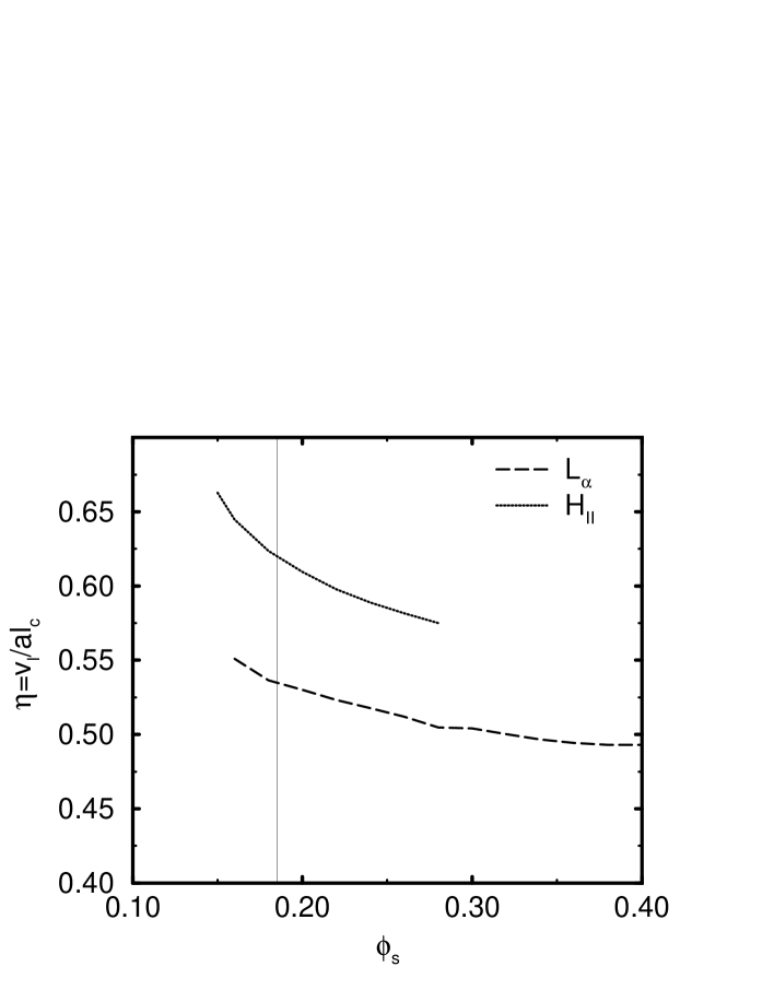
Figure 5: Packing parameter for the lamellar $L_{\alpha}$ and inverted-hexagonal $H_{II}$ phase as a function of the solvent concentration for $1/\chi=0.25$. The vertical line marks solvent composition at which the transition occurs.

References

- [1] V. Luzatti, A. Tardieu, T. Gulik-Krzywicki, E. Rivas, and F. Reiss-Husson, Nature 220, 485 (1968).
- [2] P.R. Cullis, M.J. Hope, B. de Kruijff, A.J. Verkleij, and C.P.S. Tilcock, Phospholipids and Cellular Regulation, vol 1, J.F. Kuo ed. (CRC Press, Boca Raton, 1985).
- [3] J.M. Seddon, and R.H. Templer, Phil. Trans. R. Soc. Lond. A 344, 377 (1993).
- [4] J.M. Seddon, Biochimica et Biophysica Acta 1031, 1 (1990).
- [5] D.P. Siegel, Biophys. J. 49, 1171 (1986).
- [6] J.M. Seddon, G. Cevc, and D. Marsh, Biochemistry 22, 1280 (1983).
- [7] S.M. Gruner, J. Phys. Chem. 93, 7570 (1989).
- [8] G.L. Kirk and S.M. Gruner, J. Physique 46, 761 (1985). G.L. Kirk, S.M. Gruner, and D.L. Stein, Biochemistry 23, 1093 (1984).
- [9] J. Briggs and M. Caffrey, Biophysical J. 67, 1594 (1994).
- [10] J. Briggs, H. Chung, and M. Caffrey, J. Phys. II France 6, 723 (1996).
- [11] J. Israelachvili , Intermolecular & Surface Forces, 2nd ed. (Academic, London, 1992).
- [12] G. Cevec and D. Marsh, Phospholipid Bilayers, (Wiley, New York, 1987).
- [13] K. Larson J. Chem. Phys. 93, 7304 (1989); D.C. Turner, Z.-G. Wang, S.M. Gruner, D.A. Mannock, and R. N. McElhaney, J. Phys. II France 2, 2039 (1992).
- [14] H. Heller, M. Schaefer, and K. Schulten, J. Phys. Chem. 97, 8343 (1993); K.V. Damodaran, and K.M. Merz, Biophys. J. 66, 1076 (1994); D.P. Tieleman, and H.J.C. Berendsen, J. Chem. Phys. 105, 4871 (1996).
- [15] S. Marcelja, Biochimica et Biophysica Acta 367, 165 (1974).
- [16] D.W.R. Gruen, Biochimica et Biophysica Acta 595, 161 (1981); Chem. Phys. Lipids 30, 105 (1982); J. Phys. Chem. 89, 146 (1985).
- [17] I. Szleifer, A. Ben-Shaul, and W.M. Gelbart, J. Chem. Phys. 85, 5345 (1986); A. Ben-Shaul, I. Szleifer, and W.M. Gelbart, J. Chem. Phys. 83, 3597 (1985); I. Szleifer, D. Kramer, A. Ben-Shaul, W.M. Gelbart, and S.A. Safran, J. Chem. Phys. 92, 6800 (1990); D.R. Fattal, and A. Ben-Shaul, Physica A 220, 192 (1995).
- [18] P.J. Flory, Statistical Mechanics of Chain Molecules, (Wiley-Interscience, New York, 1969). W.L. Mattice and U.W. Suter, Conformational Theory of Large Molecules: the Rotational Isomeric State Model in Macromolecular Systems, (Wiley-Interscience, New York, 1994).
- [19] L. Steenhuizen, D. Kramer, and A. Ben-Shaul, J. Phys. Chem. 95, 7477 (1991).
- [20] For a real-space approach to this phase in polymer systems in the strong-segregation limit, see H. Xi and S.T. Milner, Macromolecules 29, 2404 (1996).
- [21] M.W. Matsen and M. Schick, Phys. Rev. Lett. 72, 2660 (1994).
- [22] M.W. Matsen, Phys. Rev. Lett. 74, 4225 (1995).
- [23] M. Müller and M. Schick, Macromolecules 27, 8900 (1996).
- [24] S.T. Hyde, and S. Andersson, Z. Kristallographie 168, 213 (1984); K. Larsson, Nature 304, 664 (1983); W. Longley, and J. McIntosh, Nature 303, 612 (1983).
- [25] J.M. Seddon, G Cevc, R.D. Kaye, and D. Marsh, Biochemistry 23, 2634 (1984).
- [26] F.A.M. Leermakers and J.M.H.M. Scheutjens, J. Chem. Phys. 89, 3264 (1988).