Effect of the Tunneling Conductance on the Coulomb Staircase

Abstract

Quantum fluctuations of the charge in the single electron box are investigated. The rounding of the Coulomb staircase caused by virtual electron tunneling is determined by perturbation theory up to third order in the tunneling conductance and compared with precise Monte Carlo data computed with a new algorithm. The remarkable agreement for large conductance indicates that presently available experimental data on Coulomb charging effects in metallic nanostructures can be well explained by finite order perturbative results.

Coulomb blockade effects in metallic nanostructures are well understood in the region of low temperatures and for small tunneling conductance $G_{T}\ll G_{K}=e^{2}/h$ [1]. Recently, several groups have started to investigate in detail the breakdown of charging effects. High-temperature anomalies due to weak Coulomb blockade have been studied [2, 3, 4, 5, 6, 7, 8], and progress in fabrication techniques has lead to reliable experimental data for systems with a tunneling conductance of several $G_{K}$ [7, 8, 9, 10]. Most of the theoretical work on Coulomb blockade for strong tunneling can roughly be divided into two groups. On the one hand, a significant body of work restricts the theory to usually two charge states [11, 12, 13]. This requires the introduction of an arbitrary cut-off that enters the final results and deranges the comparison with experimental findings. On the other hand, systematic perturbative calculations in powers of the tunneling Hamiltonian $H_{T}$ can be shown [14] to be independent of the electronic bandwidth and give results in terms of experimentally measurable quantities. While this latter approach was successful [15, 16] in explaining some of the recent data on strong tunneling in the single electron transistor [10], the range of validity of perturbative results is not known a priori. In this Letter, we focus on the simplest system displaying charging effects, the single electron box. Perturbative results up to sixth order in $H_{T}$ are derived and compared with Monte Carlo data. We shall demonstrate that perturbation theory indeed does remarkably well.

FIG. 1.: Circuit diagram of the single electron box, consisting of a tunnel junction in series with a capacitor.

The circuit diagram of the single electron box in Fig. 1 shows a tunnel junction with capacitance $C_{T}$ and tunneling conductance $G_{T}$ in series with a capacitance $C_{G}$ biased by a voltage source $U_{\rm ex}$. Provided the tunneling conductance $G_{T}\ll G_{K}$, the island charge $q$ is quantized, i.e. $q=-ne$, where $n$ is the number of excess electrons in the box. At zero temperature, $n$ is a staircase function of the external voltage $U_{\rm ex}$. This idealized behavior is modified at finite temperatures, where the occupation of higher charge levels leads to a smearing of the staircase [17]. Furthermore, the finite tunneling conductance causes a hybridization of the lead and island electronic states so that the island charge is no longer strictly quantized. Since the range of validity of perturbative results is most restricted at zero temperature, we focus attention here on this case.

At zero temperature, the ground state energy ${\cal E}$ as a function of $n_{\rm ex}=C_{G}U_{\rm ex}/e$ determines the average island charge

$$\langle n\rangle=n_{\rm ex}-\frac{1}{2E_{c}}~{}\frac{\partial{\cal E}}{\partial n_{\rm ex}}~{}~{}.$$ (1)

Here $E_{c}=e^{2}/2C$ is the classical charging energy, where the island capacitance $C$ is the sum of the capacitance $C_{T}$ of the tunnel junction and the gate capacitance $C_{G}$, cf. Fig. 1. Formally ${\cal E}$ may be written as a perturbation series in powers of the tunneling conductance, leading to a diagrammatic representation of ${\cal E}$ [14]. The zeroth order term of the ground state energy for vanishing electron tunneling is determined by the minimum of the electrostatic energy and reads ${\cal E}_{0}=E_{c}(n_{0}-n_{\rm ex})^{2}$ where $n_{0}$ is the integer closest to $n_{\rm ex}$. Hence, as function of the applied voltage, the island charge displays the well known Coulomb staircase $\langle n\rangle=n_{0}$. Because of the periodicity and antisymmetry of $\langle n\rangle$ as a function of $n_{\rm ex}$, we may confine ourselves to $0\leq n_{\rm ex}<{\scriptstyle\frac{1}{2}}$.

Since the tunneling Hamiltonian $H_{T}$ transfers an electron from the lead to the island electrode or vice versa, it has no diagonal components in the basis of unperturbed energy eigenstates and only even orders in $H_{T}$ contribute to the perturbation series of ${\cal E}$. The second order term gives a contribution proportional to the dimensionless conductance $\alpha=G_{T}/G_{K}$ and is represented by the two diagrams shown in Fig. 2a. The arc to the right describes the formation of a virtual electron-hole pair in the intermediate state with an excess electron on the island, that is $n=1$, and a hole in the lead electrode. The second diagram describes the corresponding process with an intermediate state of reduced island charge $n=-1$. In the interval $0\leq n_{\rm ex}<{\scriptstyle\frac{1}{2}}$ considered, the two diagrams give a contribution to the average island charge of the form [11, 18]

$$\langle n\rangle_{1}=g\ln\frac{1+2n_{\rm ex}}{1-2n_{\rm ex}},$$ (2)

where $g=\alpha/4\pi^{2}$. The contribution of fourth order in $H_{T}$ follows from the diagrams depicted in Fig. 2b. Here the first eight diagrams describe processes with two intermediate electron-hole pairs created and annihilated in all possible ways. The remaining diagrams have a lower order diagram inserted, as indicated by the prolongation of the arc across the vertical line. These diagrams correspond to terms in the Rayleigh-Schrödinger perturbation series with energy denominators squared. Each of the arcs depicts an integral over the energy of a virtual electron-hole pair with a spectral density which becomes linear in the infinite bandwidth limit. An element of the vertical line corresponds to an energy denominator describing the energy difference between the intermediate virtual state and the ground state. The diagrammatic rules are explained in detail in [14] and it was shown there that although each single diagram diverges in the infinite bandwidth limit, the sum of all diagrams of a given order remains finite. The contribution of second order in $\alpha$ to the average island charge reads [19]

$$\begin{array}[]{rl}\langle n\rangle_{2}&=-g^{2}\Big{\{}n_{\rm ex}\left[\frac{4\pi^{2}}{3}+\ln^{2}\left(\frac{1-2n_{\rm ex}}{1+2n_{\rm ex}}\right)\right]\\ &+\frac{16(1+2n_{\rm ex}-2n_{\rm ex}^{2})}{(3-2n_{\rm ex})(1+2n_{\rm ex})}\ln(1-2n_{\rm ex})\\ &+2(1-n_{\rm ex})\Big{[}\ln^{2}\left(\frac{1-2n_{\rm ex}}{4(1-n_{\rm ex})}\right)+2\mbox{Li}_{2}\left(\frac{3-2n_{\rm ex}}{4(1-n_{\rm ex})}\right)\\ &-\frac{8(1-n_{\rm ex})}{(1-2n_{\rm ex})(3-2n_{\rm ex})}\ln(4(1-n_{\rm ex}))\Big{]}-\mbox{s.t.}(-n_{\rm ex})\Big{\}}.\end{array}$$ (3)

Here $\mbox{s.t.}(-n_{\rm ex})$ stands for the same sum of terms with $n_{\rm ex}$ replaced by $-n_{\rm ex}$ showing explicitly the asymmetry of $\langle n\rangle$ in the applied voltage $U_{\rm ex}$. Further, $\mbox{Li}_{2}(x)=-\int_{0}^{x}\mbox{d}z~{}\ln(1-z)/z$ denotes the dilogarithm function [20].

In third order in $\alpha$, one has to evaluate $160$ diagrams, some of which are shown in Fig. 2c. There are $80$ diagrams without insertions, such as the left diagram in Fig. 2c, $64$ diagrams with one insertion, and $16$ diagrams with two insertions. Using the diagrammatic rules, we have to deal with three-fold energy integrals of rational kernels. These integrals can be done analytically leading to polylogarithms [20] and powers of logarithms of rational arguments. Since the full analytic expression is rather involved [21], we present explicitly only results for two limiting cases $n_{\rm ex}\rightarrow 0$ and $n_{\rm ex}\rightarrow{\scriptstyle\frac{1}{2}}$.

FIG. 2.: Diagrams for the ground state energy in a) first order, b) second order, and c) selected diagrams in third order in $\alpha$.

For small external voltage, the average island charge grows linearly as

$$\langle Q\rangle=e\langle n\rangle=C^{*}U_{\rm ex}$$ (4)

where $C^{*}$ is an effective capacitance of the box. In the absence of Coulomb blockade effects $C^{*}=C_{G}$, while for strong Coulomb blockade, i.e., in the limit of vanishing tunneling conductance, $C^{*}=0$. It is thus natural to characterize the strength of the Coulomb blockade effect by an effective charging energy $E_{c}^{*}$ defined by [22]

$$\frac{E_{c}^{*}}{E_{c}}=1-\frac{C^{*}}{C}=1-\left.\frac{\partial\langle n\rangle}{\partial n_{\rm ex}}\right|_{n_{\rm ex}=0}.$$ (5)

The perturbation series gives

$$\frac{E_{c}^{*}}{E_{c}}=1-4g+Ag^{2}-Bg^{3}+{\cal O}(g^{4}),$$ (6)

where $A=5.066...$ and $B=1.457...$ are analytically known coefficients whose explicit form is too lengthy to present here.

The perturbation series is well behaved in the region of interest, except in the vicinity of $n_{\rm ex}={\scriptstyle\frac{1}{2}}$, where logarithmic divergences arise. This unphysical behavior indicates the failure of perturbation theory due to the degeneracy of the ground state in this limit. For $n_{\rm ex}\rightarrow{\scriptstyle\frac{1}{2}}$ one finds from the analytical expression for the average island charge

$$\langle n\rangle = ag^{2}+bg^{3}-(g+6g^{2}+cg^{3})\ln\delta$$ (8)

$$-(2g^{2}+24g^{3})\ln^{2}\delta-4g^{3}\ln^{3}\delta+{\cal O}(\delta)$$

where $\delta={\scriptstyle\frac{1}{2}}-n_{\rm ex}$, and where the coefficients $a$, $b$, and $c$ read numerically $a=-9.7726...$, $b=-70.546...$, and $c=65.462...$ . The leading order logarithmic terms in Eq. (8) are $-g\ln\delta-2g^{2}\ln^{2}\delta-4g^{3}\ln^{3}\delta$. These terms come from the diagrams shown in Fig. 3, where all intermediate states are confined to the two charge states $n=0$, $1$ which are degenerate at $n_{\rm ex}={\scriptstyle\frac{1}{2}}$. The most divergent logarithmic term of order $k$ reads $-{\scriptstyle\frac{1}{2}}(2g\ln\delta)^{k}$, and we get by resummation

$$\langle n\rangle=\frac{-g\ln\delta}{1-2g\ln\delta}.$$ (9)

This result was previously derived by Matveev [11] using renormalization group techniques.

FIG. 3.: Diagrams of order $\alpha^{k+1}$ for the ground state energy giving leading order logarithms.

To explore the range of validity of these higher order perturbative results we have carried out precise Quantum Monte Carlo (QMC) simulations for the single electron box. In contrast to earlier attempts [12, 22, 23], we do not work in the phase representation, but simulate configurations directly in the charge representation, keeping track of all intermediate electron-hole pairs. A general numeric scheme for evaluating series of integrals directly in the continuum, i.e., without invoking artificial discretization of the integration variables was explained in [24, 25]. It is possible then to develop an exact (without systematic errors) QMC algorithm summing diagrammatic series [26]. Here, the integration variables are imaginary times of charge transfer events, and we have employed this “diagrammatic” QMC for summing all graphs for the partition function [14]. The efficiency of the new algorithm has allowed us to simulate the single electron box at extremely low temperatures ($\beta E_{c}$ as large as $10^{4}$). While in the phase representation $n_{\rm ex}\neq 0$ results in a sign problem, in the charge representation all contributions are positive definite even at finite external voltage. This has enabled us to obtain for the first time QMC data for the entire staircase function.

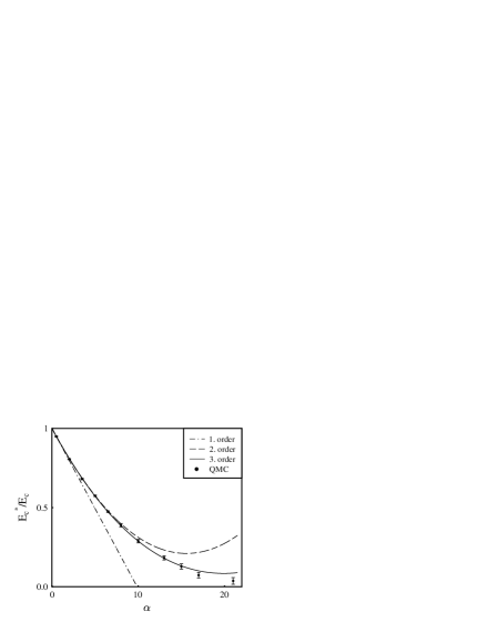
FIG. 4.: Effective charging energy as a function of the dimensionless conduction $\alpha=G_{T}/G_{K}$. Perturbative results are compared with QMC data.

In Fig. 4, the effective charging energy $E_{c}^{*}$ at zero temperature is shown as a function of the dimensionless conductance $\alpha$. Apart from the point for $\alpha=21$, the QMC data are consistent with previous results by Wang et al. [22], obtained with a different algorithm. For small external voltages, the analytical result to second order in $\alpha$ is correct with errors below $4\%$ for values of the dimensionless conductance up to $\alpha\approx 8$, while the third order result extends to $\alpha\approx 16$.

The range of validity of perturbation theory shrinks with increasing external voltage and is worst near $n_{\rm ex}={\scriptstyle\frac{1}{2}}$. In Fig. 5, the rounded Coulomb staircase is depicted for $\alpha=5$ and $\alpha=10$. While the analytical result diverges at $n_{\rm ex}={\scriptstyle\frac{1}{2}}$, we find that third order perturbation theory in $\alpha$ remains valid with errors below $4\%$ up to $n_{\rm ex}\approx 0.495$ for dimensionless conductance $\alpha=2$ (data not shown), up to $n_{\rm ex}\approx 0.45$ for $\alpha=5$, and up to $n_{\rm ex}\approx 0.4$ for $\alpha=10$. Since for $n_{\rm ex}=0.45$ the charging energies for $n=0$ and $n=1$ differ only by $0.1E_{c}$, deviations from the third order result in $\alpha$ can be observed only for temperatures well below $E_{c}/10k_{B}$ even at $n_{\rm ex}={\scriptstyle\frac{1}{2}}$. Finally, Fig. 5 shows that the resummation of the leading logarithmic terms (9) does not suffice to describe the behavior near $n_{\rm ex}={\scriptstyle\frac{1}{2}}$. Subleading logarithms are important to obtain quantitatively meaningful results.

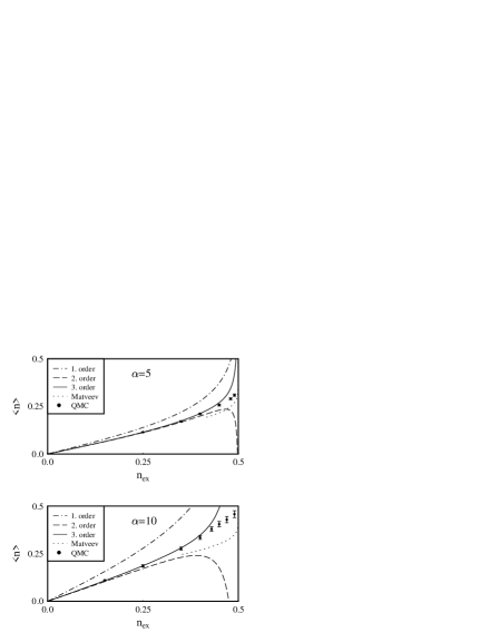
FIG. 5.: The average electron number $\langle n\rangle$ as a function of the dimensionless voltage $n_{ex}$ is shown in first, second, and third order perturbation theory in $\alpha$, and compared with QMC data. The result (8) is also shown as a dotted line.

In summary, we have studied the breakdown of Coulomb charging effects with increasing tunnel conductance. Precise Monte Carlo data for the effective charging energy as well as for the smeared staircase function were presented. Comparing analytical results with these data, the range of validity of expansions in powers of the tunneling conductance was determined. It was found that presently attainable experimental results are covered by expansions up to third order in $\alpha$. With increasing $\alpha$, the effective charging energy $E_{c}^{*}$ decreases rapidly. Since finite temperature corrections for large $\alpha$ are controlled by the dimensionless parameter $\beta E_{c}^{*}$[22], experiments with dimensionless conductance above $\alpha=10$, where perturbation theory begins to fail, require extremely low temperatures to see nonperturbative effects. We finally mention that the methods employed here can be extended to other systems displaying charging effects, such as the single electron transistor.

The authors would like to thank M.H. Devoret, D. Esteve, P. Joyez, J. König, and H. Schoeller for valuable discussions. H.G. and N.P. acknowledge hospitality and support by the Institute for Nuclear Theory, Washington University, Seattle, where this work was started. Additional support was provided by the Deutsche Forschungsgemeinschaft (Bonn) and the Russian Foundation for Basic Research.

REFERENCES

- [1] Single Charge Tunneling, H. Grabert, M.H. Devoret (eds.), NATO ASI Series B, Vol. 294 (Plenum, NY, 1992).
- [2] J.P. Pekola, K.P. Hirvi, J.P. Kauppinen, and M.A. Paalanen, Phys. Rev. Lett. 73, 2903 (1994).
- [3] G. Göppert, Diploma thesis, Freiburg 1996.
- [4] D.S. Golubev and A.D. Zaikin, JETP Lett. 63, 1007 (1996).
- [5] G. Göppert, X. Wang, and H. Grabert, Phys. Rev. B 55, R10213 (1997).
- [6] P. Joyez and D. Esteve, Phys. Rev. B 56, 1848 (1997).
- [7] J.J. Toppari, Sh. Farhangfar, Yu.A. Pashkin, A.J. Manninen, J.P. Pekola, X.H. Wang, and K.A. Chao (preprint)
- [8] P. Joyez, D. Esteve, and M.H. Devoret, Phys. Rev. Lett. 80, 1956 (1998).
- [9] J.P. Kauppinen and J.P. Pekola, Phys. Rev. Lett. 77, 3889 (1996).
- [10] P. Joyez, V. Bouchiat, D. Esteve, C. Urbina, and M. H. Devoret, Phys. Rev. Lett. 79, 1349 (1997).
- [11] K.A. Matveev, Sov. Phys. JETP 72, 892 (1991).
- [12] G. Falci, G. Schön, and G.T. Zimanyi, Phys. Rev. Lett. 74, 3257 (1995).
- [13] H. Schoeller and G. Schön, Phys. Rev. B 50, 18436 (1994).
- [14] H. Grabert, Phys. Rev. B 50, 17364 (1994).
- [15] J. König, H. Schoeller, and G. Schön, Phys. Rev. Lett. 78, 4482 (1997).
- [16] J. König, H. Schoeller, and G. Schön, preprint, cond-mat/9801214
- [17] P. Lafarge, et al., Z. Phys. B 85, 327 (1991).
- [18] D. Esteve, in Ref. [1], Single Charge Tunneling.
- [19] H. Grabert, Physica B 194-196, 1011 (1994).
- [20] L. Lewin, Polylogarithms and associated functions (North-Holland, NY, 1981).
- [21] G. Göppert and H. Grabert, to be published.
- [22] X. Wang, R. Egger, and H. Grabert, Europhys. Lett. 38, 545 (1997).
- [23] W. Hofstetter and W. Zwerger, Phys. Rev. Lett. 78, 3737 (1997).
- [24] N.V. Prokof’ev, B.V. Svistunov, and I.S. Tupitsyn, Pis’ma v Zh. Eksp. Teor. Fiz. 64, 853 (1996); [Sov. Phys. JETP Lett. 64, 911].
- [25] N.V. Prokof’ev, B.V. Svistunov, and I.S. Tupitsyn, to appear in Zh. Eksp. Teor. Fiz.; cond-mat/9703200.
- [26] N.V. Prokof’ev and B.V. Svistunov, to be published.