[

Numerical Study of the Three-Dimensional Gauge Glass Model

Abstract

We investigate numerically the finite-size scaling properties of the domain wall energies in the three-dimensional gauge glass model. From the analysis of results obtained for systems of linear sizes $3\leq L\leq 8$ we conclude that the stiffness exponent of the model is positive. This implies the existence of a stable ordered phase at low but finite temperatures.

]

It has been suggested that in type-II superconductors at low temperatures defects may pin the flux lines at random positions thus destroying the Abrikosov vortex lattice. This leads to a new type of superconducting state, the vortex glass[1, 2], in which the phase of the superconducting order parameter is random in space but frozen in time, much in the same way magnetic moments are frozen in the low-temperature phase of spin glasses. The simplest system expected to have an ordered phase analogous to the vortex glass is the gauge glass model, originally introduced to describe disordered arrays of Josephson junctions in an external magnetic field[3, 4]. This model is defined by the Hamiltonian

$$H=-J\sum_{ij}\cos\left(\theta_{i}-\theta_{j}-A_{ij}\right),$$ (1)

where $\theta_{i}$ is the phase of the order parameter at the $i$-th site of a simple cubic lattice and the sum runs over all pairs of neighboring sites. The energy scale is set by the coupling constant $J$ and the lattice spacing is identified with the typical distance between vortices[5]. The phase shifts $A_{ij}=(2\pi/\Phi_{0})\int_{i}^{j}\vec{A}\cdot d\vec{l}$ where $\vec{A}$ is the vector potential of the applied magnetic field and $\Phi_{0}$ the flux quantum. The effects of the disorder in the positions of the vortices are incorporated by taking the phase shifts as independent quenched random variables. The situation that interests us, where the disorder and the external field are large, may be modeled by taking $A_{ij}$ uniformly distributed in the interval $[0,2\pi]$. The three-dimensional gauge glass model has been extensively studied numerically by Monte Carlo simulation [6, 7, 8] and finite-size scaling of defect wall energies [7, 9, 10] the important issue being whether a thermodynamically ordered phase can exist at finite temperature in this system. Although the results of the earlier Monte-Carlo studies[6, 7] of the model were consistent with the existence of a low-temperature vortex glass phase, they could not rule out a zero-temperature transition since only small systems could be brought to equilibrium below $T\sim 0.6J$. Stronger evidence in favor of a finite-temperature transition has been obtained in recent simulations based on the vortex representation of the problem[8] in which it was found that the transition temperature may be as high as $T_{\rm c}=0.93J$. On the other hand, the domain-wall renormalization-group (DWRG) studies performed so far [7, 9, 10] were inconclusive, the sizes of the systems studied being too small and the statistical error too large to decide unambiguously whether the lower critical dimension of the model is above or below three. In this paper we reexamine this problem by means of a DWRG study of model (1) with an algorithm that we have recently proposed and applied to the $XY$ spin-glass model in three dimensions[11]. This algorithm allows us to study lattices substantially bigger than with conventional methods as well as to improve upon the statistics. In the defect wall method[12, 13] the energy cost $W$ of introducing a domain wall in the system is studied as a function its linear size $L$. In the scaling regime one finds [12, 13] $W\sim L^{\theta}$ where the stiffness exponent $\theta$ may be positive or negative depending on whether the system is above or below its lower critical dimension $d_{\rm c}$. From the results obtained for our five largest sizes ($4\leq L\leq 8$) we find the value $\theta_{\rm GG}=0.077\pm 0.011$ for the gauge glass model. This result implies that a stable ordered phase exists at low but finite temperatures.

To determine the domain-wall energy one computes the differences $\Delta E=E_{\rm P}-E_{\rm A}$ between the ground-state energies corresponding to periodic (P) and anti-periodic (AP) boundary conditions along some direction for an ensemble of systems of size $N_{\rm s}=L^{3}$. The boundary conditions along the two remaining directions are kept fixed. For sufficiently large systems the distribution of energy differences differences ${\cal P}(\Delta E,L)$ is expected to have the scaling form[13]

$${\cal P}(\Delta E,L)=L^{-\theta}\tilde{{\cal P}}(\Delta EL^{-\theta}).$$ (2)

The width of the distribution, $W(L)=\langle\Delta E^{2}\rangle_{A_{ij}}^{1/2}\sim L^{\theta}$, is interpreted as the effective coupling constant between blocks of $N_{\rm s}$ sites[12, 13, 14]. If $\theta>0$, the rigidity of a block diverges with its size, which indicates that the system has long-range order. If the stiffness exponent is negative, the correlation length diverges at $T=0$ with $\xi\sim T^{-\nu}$ and $\nu=1/|\theta|$ [14].

The ground state of the gauge glass model is given by the absolute minimum of (1) subject to the appropriate boundary conditions. In the presence of disorder the extremal conditions $\partial H/\partial\theta_{i}=0\ \forall i$ have in general a very large number of solutions whose presence greatly complicates the task of searching that with the lowest energy. In the spin-quench algorithm[15](SQA) usually employed to solve this type of problem, long sequences of metastable states are randomly generated among which one will find the ground-state provided the number of trials is sufficiently large. Since the number of metastable states of a frustrated system increases exponentially with its size[14], so does the number of trials required. This limits the maximum size of the systems that can be studied using this method in practice. We have recently proposed a far more efficient algorithm for the search of ground states[11]. It is based upon the morphological characteristics of the low-lying states of frustrated $XY$ models as revealed by detailed examination of numerous examples[16]. For a given realization of the disorder in Eq.1, the low-energy configurations are characterized by the existence of regions where the order parameter varies smoothly (domains), and others where the spatial distribution of the phases looks pretty much random. The former exist in parts of the sample where frustration is low, the latter where it is high. As it turns out[16], the position, size and shape of the domains are mostly determined by the realization of the disorder and are essentially the same for all the low-energy states. Aside from smooth distortions of the order parameter, the essential differences between any two such states are almost rigid rotations of the individual domains, accompanied by large amplitude rearrangements of the phases in the frustrated regions between them. Stationary states in which the domain structure is disrupted do exist, but their energy is much higher. In our method, sequences of low-energy configurations are generated recursively in such a way that the domain structure is preserved at each step. The result is a reduction of the probability of appearance of high-energy configurations in the sequence and a corresponding enhancement of that of finding the ground-state or states lying nearby in energy. The procedure is as follows [11]. The first state in the sequence, $\{\theta^{(0)}\}$, is obtained by a conjugate-gradient minimization (CGM) of the energy (1) starting from a random distribution of phases. New states are generated by iterating the following steps. i) Sites are divided in two classes according to whether the ‘local field’ $h_{i}=-J\sum_{j}\cos\left(\theta_{i}-\theta_{j}-A_{ij}\right)$ in the $n$-th configuration $\theta^{(n)}$is greater or smaller than a threshold value $h_{\rm t}$ chosen as explained below. The sites in the first group constitute the domains. ii) Correlations between the domains and the rest of the system are destroyed by a random rigid rotation of the former. iii) A fraction $p$ of the $N_{\rm w}$ sites in weak local fields are picked at random and their phases reset to arbitrary values. iv) The energy of the subsystem formed by the domains is minimized with the phases on the remaining sites fixed. v) The state resulting from the previous step is allowed to relax by performing a CGM of the total energy of the system. The outcome is the next state in the sequence, $\{\theta_{\rm n+1}\}$. vi) The energy of this state is stored and, eventually, $h_{\rm t}$ is rescaled.

The efficiency of this algorithm depends upon the chosice of the parameters $h_{\rm t}$ and p. The threshold field fixes the degree of homogeneity required of a region for it to be classified as a domain. If it is too high or if $p$ is too large, too many sites are involved in step iii) and the domain structure is disrupted just as in the SQA where all the phases are randomly reset at each step.

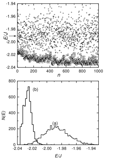
FIG. 1.: Upper panel : Energies of some of the metastable states of a realization of the gauge glass model on a 512-site 3D lattice. Results are plotted as a function of iteration number for the spin quench algorithm (crosses) and for our algorithm (squares). The arrow indicates the energy of the first state in our sequence. Lower panel : Distribution of the energies of two series of 5 000 metastable states each obtained with the SQA (a) and with our algorithm (b).

If, on the contrary, $h_{\rm t}$ or $p$ are too small, the algorithm gets trapped in phase space and all the states in the sequence are close to the initial one. The two parameters must therefore be continuously readjusted in the course of the simulation to ensure good performances. We have empirically found that the algorithm performs at its best for large samples when the number of sites involved in step iii) $pN_{\rm w}\equiv n\sim 0.05N_{\rm s}$. If at some stage of the iteration $N_{\rm w}<n$ we consider that the threshold field is too low and too many sites are being included in the domains. We then rescale it upwards, $h_{\rm t}\to(1+\alpha)\ h_{\rm t}$ with $\alpha\sim 0.05$, and we randomly reset the phases on all the sites where the local field is weak. If $n\leq N_{\rm w}\leq 2n$, $h_{\rm t}$ is unchanged and the phases are updated on just $n$ randomly chosen sites. Finally, if $N_{\rm w}>2n$ we consider that the threshold field is too high and we rescale it downwards according to $h_{\rm t}\to(1-\alpha)\ h_{\rm t}$. We find that, in practice, the field stabilizes itself after a few iterations and oscillates about a value that, in the case of the simulations reported here, is $\sim 2.6J$.

In the upper panel of Fig.1 we show the energies of two series of 1000 minima of (1) for a particular realization of the disorder. Data were obtained for a 3D lattice of $512$ sites using periodic boundary conditions. The crosses represent states obtained with the SQA and the squares are the outcome of the first thousand iterations of our algorithm. The arrow points at the energy of the first configuration of our sequence. It can be seen that, whereas the conventional algorithm randomly samples the whole of phase space, our method seems to mostly explore the deepest valleys. Notice that during the first five hundred or so iterations the typical energy of the states in the sequence decreases continuously after which it stabilizes in a region of energies that is hardly ever visited by the SQA. It is important to check that the configurations that enter in the sequence come from well separated regions of phase space rather than from a particular valley where the algorithm would be trapped. This may be done simply by monitoring the evolution of the overlap of the successive configurations with a particular one that is chosen as reference. The lower panel of Fig.1 shows histograms obtained after five thousand iterations of the two algorithms. It can be seen that the histogram obtained with our method is much narrower and centered at a much lower energy. The overall features of the distribution of energies shown in Fig.1 are quite similar to those recently found for the $\pm J$ spin glass model[11]. It is remarkable that about twenty percent of the states found using our algorithm in this example have never been generated by the SQA. Our lowest energy state, at $E=-2.036J$, appears $\sim 200$ times in the sequence. The configurations of the states that have this energy are related to each other by uniform rotations. In between them, the algorithm generates states that are in far away regions of phase space. We believe that this state is the ground state of this particular realization.

In order to study the scaling properties of defects energies in the gauge glass model we have applied the above method to compute ground-state energies with periodic and antiperiodic boundary conditions for systems of $L^{3}$ sites with $3\leq L\leq 8$. Only systems with $L\leq 5$ had been investigated previously[9, 10] . We generated sequences of states containing 500 ($L$=3), 800 ($L$=4), 1000 ($L$=5), 2000 ($L$=6), 3000 ($L$=7) and 5000 ($L$=8) elements, respectively. Disorder averages were taken over 25600 ($L$=3), 6400 ($L$=4), 2560 ($L$=5,6), 640 ($L$=7) and 256 ($L$=8) samples, respectively. The normalized distributions of the differences $\Delta E=|E_{\rm P}-E_{\rm AP}|$ obtained numerically for the different sizes are shown in Fig.2. Detailed examination of the results shows that the differences between the curves for different sizes are of the same order of magnitude as the statistical error bars. Because of this we were not able to determine the stiffness exponent of the model by performing a scaling plot as Eq.2 suggests.

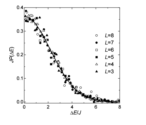
FIG. 2.: Probability distributions of the differences of the ground-state energies with periodic and antiperiodic boundary conditions. The solid line is the result of a gaussian fit of the ensemble of the data.

The solid curve in the Fig.2 is a gaussian of width $W=2.25J$. The fact that we can quite reasonably describe the ensemble of the data using a single size-independent distribution is an indication that the lower critical dimension of the gauge glass problem is very close to three, as found by other authors[7, 9, 10]. The $L$-dependence of the effective coupling $W(L)=\langle\Delta E^{2}\rangle_{A_{ij}}^{1/2}$ is shown in the log-log plot of Fig.3. As the figure shows, statistics for the two largest systems is still unsatisfactory but very hard to improve upon because of CPU-time limitations. Nevertheless, we can still conclude from the available data that the domain-wall energy increases slowly with length scale. Leaving out the point for $L=3$ which is likely to be too small a size for scaling to hold, we can make a power-law fit of the results. The stiffness exponent thus determined is $\theta_{\rm GG}=0.077\pm 0.011$. We have checked this result by repeating the calculation for the larger sizes starting from different random initial configurations. The differences found between the results thus obtained fall within the statistical error bar. Our value for the stiffness exponent is consistent with those reported by Gingras[9]($\theta_{\rm GG}=0.04\pm 0.06$) and by other authors[7, 10] who find $\theta_{\rm GG}\approx 0$ within their statistics. Ours is, to our knowledge, the first calculation in which the possibility $\theta_{\rm GG}\leq 0$ is outside the range covered by the error bar.

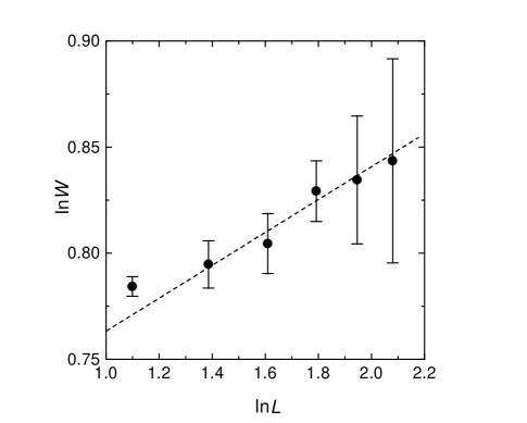
FIG. 3.: The $L$-dependence of the domain-wall energies for the gauge glass model on $L\times L\times L$ simple cubic lattices. The dashed line is the power-law fit discussed in the text.

The results of this paper thus confort the idea that the lower critical dimension of the gauge glass model is slightly below three. The implication is that the system has a finite-temperature transition to an ordered state in agreement with the findings of the Monte Carlo studies of the model[6, 7, 8]. It is interesting to notice that whereas the smallness of $\theta_{\rm GG}$ would lead one to naively expect a very low transition temperature, the Monte Carlo data indicate that $T_{\rm c}\sim{\cal O}(J)$. This is a somewhat puzzling result that deserves further investigation.

The calculations presented here have been done on a 256-processor CRAY T3E parallel computer at the ‘Centre Grenoblois de Calcul Vectoriel’. We thank the staff for their technical help.

REFERENCES

- [1] M. P. A. Fisher, Phys. Rev. Lett. 62, 1415 (1989).
- [2] D. S. Fisher, M. P. A. Fisher and D. A. Huse, Phys. Rev. B 43, 130 (1991).
- [3] C. Ebner and D. Stroud, Phys. Rev. B 31, 165 (1985).
- [4] E. Granato and J. M. Kosterlitz, Phys. Rev. B 33, 6533 (1986); Phys. Rev. Lett. 62, 823 (1989).
- [5] M. P. A. Fisher, T. A. Tokuyasu, A. P. Young, Phys. Rev. Lett. 66, 2931 (1991).
- [6] D. A. Huse and H. S. Seung, Phys. Rev. B 42, 1059 (1990).
- [7] J. D. Reger, T. A. Tokuyasu, A. P. Young and M. P. A. Fisher, Phys. Rev. B 44, 7147 (1991).
- [8] C. Wengel and A. P. Young, Phys. Rev. B 56, 5918 (1997).
- [9] M. J. P. Gingras, Phys. Rev. B 45, 7547 (1992).
- [10] J. M. Kosterlitz and M. Simkin, Phys. Rev. Lett. 79, 1098 (1997).
- [11] J. Maucourt and D. R. Grempel, Phys. Rev. Lett. 80, 770 (1998).
- [12] J. R. Banavar and M. Cieplak, Phys. Rev. Lett. 48, 832 (1982); M. Cieplak and J. R. Banavar, Phys. Rev. B 29, 469 (1984).
- [13] W. L. McMillan, Phys. Rev. B 31, 342 (1985).
- [14] B. M. Morris, S. G. Colborne, M. A. Moore, A. J. Bray and J. Canisius, J. Phys. C 19, 1157 (1986).
- [15] L. R. Walker and R. E. Walstedt, Phys. Rev. B 22, 3816 (1980).
- [16] P. Gawiec and D. R. Grempel, Phys. Rev. B 44, 2613 (1991).