Heating of a two-dimensional electron gas by the electric field of a surface acoustic wave

Abstract

The heating of a two-dimensional electron gas by an rf electric field generated by a surface acoustic wave, which can be described by an electron temperature $T_{e}$, has been investigated. It is shown that the energy balance of the electron gas is determined by electron scattering by the piezoelectric potential of the acoustic phonons with $T_{e}$ determined from measurements at frequencies $f$= 30 and 150 MHz. The experimental curves of the energy loss $Q$ versus $T_{e}$ at different SAW frequencies depend on the value of $\omega\bar{\tau}_{\epsilon}$, compared to 1, where $\bar{\tau}_{\epsilon}$ is the relaxation time of the average electron energy. Theoretical calculations of the heating of a two-dimensional electron gas by the electric field of the surface acoustic wave are presented for the case of thermal electrons ($\Delta T\ll T$). The calculations show that for the same energy losses $Q$ the degree of heating of the two-dimensional electrons (i.e., the ratio $T_{e}/T$) for $\omega\bar{\tau}_{\epsilon}>1$ ($f$= 150 MHz) is less than for $\omega\bar{\tau}_{\epsilon}<1$ ($f$=30 MHz). Experimental results confirming this calculation are presented.

I INTRODUCTION

The investigation of nonlinear (with respect to the input power) effects in the absorption of piezoelectrically active ultrasonic waves, arising due to the interaction of the waves with three- dimensional electron gas (in the case of Boltzmann statistics), has shown that the mechanisms of the nonlinearity depend on the state of the electrons. If electrons are free (delocalized), then the nonlinearity mechanism for moderately high sound intensities is usually due to the heating of the electrons in the electric field of an ultrasonic wave. The character of the heating depends on the quantity $\omega\tau_{\epsilon}$, where $\omega$ is the sound frequency, and $\tau_{\epsilon}$ is the energy relaxation time [1, 2]. If the electrons are localized, then the nonlinearity mechanism is due to the character of the localization (on an individual impurity or in the wells of a fluctuation potential). In [3], it was shown that in the case where the electrons are localized on individual impurities, the nonlinearity was determined by impurity breakdown in the electric field of the sound wave. When the electrons occupied the conduction band as a result of this effect, their temperature started to grow as a result of heating in the electric field of the wave [4].

The study of structures with a two-dimensional electron gas (2DEG) opens up a unique possibility of studying in one series of measurements performed on the same sample the mechanisms of nonlinearity in delocalized and localized electron states, since under quantum Hall effect conditions both states are realized by varying the magnetic field. The change in the absorption coefficient for a piezoelectrically active surface acoustic wave (SAW) interactimg with a 2DEG as a function of the SAW intensity in GaAs/AlGaAs structures was previously observed in [5] and [6] only in the magnetic field range corresponding to small integer filling numbers-the quantum Hall effect regime, when the two-dimensional electrons are localized. The authors explained the data which they obtained by heating of a 2DEG.

In the present paper we report some of our investigations concerning nonlinear effects accompanying the interaction of delocalized two- dimensional electrons with the electric field of a SAW for the purpose of investigating nonlinearity mechanisms.

II EXPERIMENTAL PROCEDURE

We investigated the absorption coefficient for a 30-210 MHz SAW in a two-dimensional electron gas in $GaAs/Al_{0.75}Ga_{0.25}As$ heterostructures as a function of the temperature in the range $T\simeq 1.4-4.2K$ in the linear regime (the input power did not exceed $10^{-7}$W) and the SAW power at $T=1.5K$ in magnetic fields up to 30 kOe. Samples studied previously in [7] with Hall density $n_{s}^{H}=6.7\cdot 10^{11}cm^{-2}$ and mobility $\mu_{H}=1.28\cdot 10^{5}cm^{2}/(Vs)$ at T=4.2 K were used for the investigations. The technology used to fabricate the heterostructures is described in [8] and the procedure for performing the sound absorption experiment is described in [7]. Here we only note that the experimental structure with 2DEG was located on the surface of the piezodielectric (lithium niobate $LiNbO_{3}$), along which the SAW propagates. The SAW was excited in a pulsed regime by sending radio pulses with filling frequency 30- 210 MHz from an rf oscillator into the excited interdigital transducer. The pulse duration was of the order of 1$\mu s$ is and the pulse repetition frequency was equal to 50 Hz. In the present paper the SAW power is the power in a pulse.

An ac electric field with the frequency of the SAW, which accompanies the deformation wave, penetrates into a channel containing two- dimensional electrons, giving rise to electrical currents and, correspondingly, Joule losses. As a result of this interaction, energy is absorbed from the wave. The SAW absorption in a magnetic field is measured in the experiment. Since the measured absorption is determined by the conductivity of the 2DEG, quantization of the electronic spectrum, which leads to Shubnikov-de Haas oscillations, gives rise to oscillations in the SAW potential as well.

III EXPERIMENTAL RESULTS AND ANALYSIS

Curves of the absorption coefficient $\Gamma$ versus the magnetic field $H$ are presented in Fig.1 for different temperatures and powers of the 30-MHz SAW. Similar curves were also obtained for other SAW frequencies. The character of the curves $\Gamma(H)$ is analyzed in [7]. The absorption maxima $\Gamma_{max}$ as a function of the magnetic field for $H<25$kOe are equally spaced as a function of $1/H$, and the splitting of the maxima $\Gamma(H)$ for $H>25$ kOe into two peaks with the values of $\Gamma_{M}$ at the maxima is due to the relaxational character of the absorption. The temperature and SAW power dependences of $\Gamma$, shown in Figs. 2 and 3, were extracted from the experimental curves of the same type as in Fig.1 for the corresponding frequencies in a magnetic field $H<25$kOe for large filling numbers $\nu=n_{s}hc/2eH>7$.

Figure 2 shows the temperature dependence of the quantity $\Delta\Gamma=\Gamma_{max}-\Gamma_{min}$ measured in the linear regime at a frequency of 150 MHz in different magnetic fields. Here $\Gamma_{max}$ and $\Gamma_{min}$ are the values of $\Gamma$ on the upper and lower lines, which envelop the oscillatory dependence $\Gamma(H)$ for $H<25$kOe. Figure 3 shows $\Delta\Gamma$ versus $P$-the power of the SAW (frequency 150 MHz) at the oscillator output at $T$=1.5K. We see from Figs. 2 and 3 that $\Delta\Gamma$ decreases with increasing temperature and with increasing SAW power.

In [7] it was shown that in the range of magnetic fields where the quantum Hall effect is still not observed (in our case $H<25$ kOe) the dissipative conductivities are

$\sigma_{XX}^{ac}=\sigma_{XX}^{dc}$,

where $\sigma_{XX}^{dc}$ is the conductivity calculated from the measured dc resistivities $\rho_{xx}(H)$ and $\rho_{xy}(H)$, and $\sigma_{XX}^{ac}$ is the conductivity found from the absorption coefficient $\Gamma(H)$ measured in the linear regime. This result gave us the basis for assuming that in this range of magnetic fields the electrons are in a delocalized state. As we have already indicated in the introduction, we shall analyze here nonlinearity only in this case.

In a previous work [9] we showed that if the electrons are delocalized, then the characteristics of the 2DEG, such as the carrier density $n_{s}$, the transport relaxation time $\tau$, and the quantum relaxation time, can be determined from the magnetic field dependences $\sigma_{XX}^{ac}(H)$. In addition, the mobility $\mu=e\tau/m$ and the concentration $n_{s}$ at $H=0$ are close to the values obtained from dc measurements: the Hall density and mobility of the electrons, as well as $n_{s}$ found from the Shubnikov-de Haas oscillations. For this reason, it was natural to assume that $\Gamma$ depends on the SAW power, just as in the static case, because of the heating of the 2DEG but in the electric field of the SAW. The heating of the 2DEG in a static electric field in similar heterostructures was investigated in [11, 12, 13, 14, 15]. In those papers it was shown that at liquid-helium temperatures the electron energy relaxation processes are determined in a wide range of 2DEG densities by the piezoacoustic electron-phonon interaction under small-angle scattering and weak screening conditions.

We shall employ, by analogy with [11, 12, 13, 14], the concept of the temperature $T_{e}$ of two- dimensional electrons and determine it by comparing the curves of the absorption coefficient $\Gamma$ versus the SAW power with the curves of $\Gamma$ versus the lattice temperature $T$. Such a comparison makes it possible to establish a correspondence between the temperature of the two- dimensional electrons and the output power of the oscillator. The values of $T_{e}$ were extracted by two methods: 1) by comparing the curves of the amplitude of the oscillations $\Delta\Gamma=\Gamma_{max}-\Gamma_{min}$ versus the temperature $T$ (Fig. 2) and versus the power $P$ (Fig. 3) for the same value of the magnetic field $H$; 2) by comparing curves of the ratios $\Gamma_{max}/\Gamma_{M}=f(T)$ and $\Gamma_{max}/\Gamma_{M}=f(P)$ versus the lattice temperature $T$ and the power $P$. Here the values of $\Gamma_{max}(T)$ and $\Gamma_{max}(P)$ were also taken for the same value of $H$, and $\Gamma_{M}$ is the absorption at $H$=28 kOe (Fig. 1). The use of the ratios instead of the absolute values of $\Gamma$ decreased the effect of the experimental variance in $\Gamma$ on the error in determining $T_{e}$. As a result, the accuracy in determining $T_{e}$ by these two methods was no worse than $10\%$.

To determine the absolute energy losses as a result of absorption of SAW in the case of interaction with electrons ($\bar{Q}$), the following calculations must be performed. The intensity $E$ of the electric field, in which the two-dimensional electrons of the heterostructure are located during the propagation of a SAW in a piezoelectric material placed at a distance $a$ from a high-conductivity channel, is

$$\ |E|^{2}=K^{2}\frac{32\pi}{\nu}(\epsilon_{1}+\epsilon_{0})\frac{bqexp(-2qa)}{1+[(4\pi\sigma_{xx}/\epsilon_{s}v)c]^{2}}W,$$ (1)

where $K^{2}$ is the electromechanical coupling constant; $\nu=3.5\cdot 10^{5}$ cm/s and $q$ are, respectively, the velocity and wave number of sound in $LiNbO_{3}$; $a$ is the width of the vacuum gap between the sample and the $LiNbO_{3}$ plate; $\epsilon_{0}$, $\epsilon_{1}$ and $\epsilon_{s}$ are the permittivities of free space, $LiNbO_{3}$, and the semiconductor with the 2DEG, respectively; and $W$ is the input SAW power scaled to the width of the sound track. The functions $b$ and $c$ are

$$b=(\epsilon_{1}^{+}\epsilon_{s}^{+}-\epsilon_{1}^{-}\epsilon_{s}^{-}\exp(-2qa))^{-2},$$ (2)

$$c=\frac{1}{2}(1+b^{1/2}[\epsilon_{1}^{+}\epsilon_{s}^{-}-\epsilon_{1}^{-}\epsilon_{s}^{+}\exp(-2qa)]),$$ (3)

$$\epsilon_{1}^{+}=\epsilon_{1}+\epsilon_{0},\epsilon_{s}^{+}=\epsilon_{s}+\epsilon_{0},$$ (4)

$$\epsilon_{1}^{-}=\epsilon_{1}-\epsilon_{0},\epsilon_{s}^{-}=\epsilon_{s}-\epsilon_{0}.$$ (5)

The magnitude of the electric losses is defined as $\bar{Q}=\sigma_{xx}E^{2}$. Multiplying both sides of Eq.(1) by $\sigma_{xx}$, we obtain $Q=4W\Gamma/n$, where $\Gamma$ is the absorption measured in the experiment. The power $W$ at the entrance to the sample is not measured very accurately in acoustic measurements. The problem is that this quantity is determined by, first, the quality of the interdigital transducers; second, by the losses associated with the mismatch of the line that feeds electric power into the transmitting transducer as well as the line that re moves electrical power from the detecting transducer, where the losses in the receiving and transmitting parts of the line may not be the same; and, third, by absorption of the SAW in the substrate, whose absolute magnitude is difficult to measure in our experiment. The effect of these losses de creases with frequency, so that in determining $W$ at 30 MHz we assumed that both the conversion losses for the transmitting and receiving transducers as well as the losses in th transmitting and receiving lines are identical. The total losses were found to be $\Delta P$=16 dB, if SAW absorption in the heterostructure substrate is ignored. If it is assumed that nonlinear effects at 150 MHz start at the same value of $\bar{Q}$ as a 30 MHz, then the ”threshold” value of $\bar{Q}$ at which the deviation of $\Gamma_{max}(\bar{Q})/\Gamma_{M}$ at 30 MHz from a constant value be comes appreciable [we recall that $\Gamma(H)/\Gamma_{M}\sim 1/\sigma_{xx}(H)$ in the region of delocalized electronic states, i.e., $H<$25 kOe [7]] can be used to determine the total losses at 150 MHz. An estimate of the total losses by this method at 150 MHz give; $\Delta P$=18 dB. Therefore, the power $W$ at the entrance to the sample is determined by the output power $P$ of the oscillator taking into account the total losses $\Delta P$.

With the results of [11, 12, 13, 14] in mind, we constructed the curves

$$Q=\bar{Q}/n_{s}=f(T_{e}^{3}-T^{3}),$$ (6)

which correspond to the energy balance equation in the cast of the interaction of electrons with the piezoelectric potential of the acoustic phonons (PA scattering) under the condition of weak screening at frequencies of 30 and 150 MHz in different magnetic fields

$$Q_{PA}=e\mu E^{2}=A_{3}(T_{e}^{3}-T^{3}).$$ (7)

But since the condition for weak screening was not satisfied for this sample, the curves $Q=f(T_{e}^{5}-T_{0}^{5})$, corresponding to the energy balance equation in the case of PA scattering but with the condition of strong screening for the same frequencies 30 and 150 MHz and the same magnetic fields, were also constructed:

$$Q_{PA}=A_{5}(T_{e}^{5}-T_{0}^{5}),$$ (8)

A least-squares analysis showed that the expression (3) gives a better description of the experimental curves. Figure 4 shows the experimental points and theoretical curves of the expressions of the type (3) with $A_{5}=3.0\pm 0.5eV/(s\cdot K^{5})$ and $f$=30 MHz, where $f$ is the SAW frequency (see curve $1$ in Fig.4), and $A_{5}=4.0\pm 0.6eV/(s\cdot K^{5})$ and $f$=150 MHz (see curve $2$ in Fig. 4).

IV THEORY OF HEATING OF TWO- DIMENSIONAL ELECTRONS WITH CONTROL OF RELAXATION ON THE LATTICE BY ELECTRON-ELECTRON COLLISIONS

To describe the heating of an electron gas by means of a temperature $T_{e}$ different from the lattice temperature $T$, the electron-electron collisions must occur more often than collisions with the lattice; i.e., the condition $\tau_{ee}<<\tau_{\epsilon}$, must be satisfied. Here $\tau_{ee}$ and $\tau_{\epsilon}$ are, respectively, the electron energy relaxation time on phonons and the electron-electron ($ee$) interaction time.

In a weakly disordered 2DEG in GaAs/AIGaAs hetero- structures, momentum is dissipated mainly on the Coulomb charge of the residual impurity near the interface. As a result, the relaxation times satisfy the inequalities

$$\tau_{p}\ll\tau_{ee}\ll\tau_{\epsilon},$$ (9)

where $\tau_{p}$ is the electron momentum relaxation time.

A Static regime

When the inequalities (4) are satisfied, the nonequilibrium part of the distribution function has the form

$$f_{p}=-e{\bf E}\cdot{\bf v}\tau_{p}\frac{\partial f_{0}(\epsilon_{p})}{\partial\epsilon_{p}},$$ (10)

where ${\bf E}$ is the electric field, ${\bf v}$ is the electron velocity, $f_{0}(\epsilon_{p})$ is the principal part of the distribution function of electrons with energy $\epsilon_{p}=p^{2}/2m$, where $p$ and $m$ are, respectively, the electron momentum and effective mass. Because of the rapid $ee$ collisions, a Fermi distribution is established for $f_{0}(\epsilon_{p})$, but the Fermi level $\epsilon_{F}$ and the temperature $T_{e}$ must be determined from the conservation equations for the electron density and average energy, while the electron-phonon collisions give rise to energy transfer from the electrons to the lattice.

The results of a calculation of the energy balance equation in a 2DEG in the case of electron scattering by piezoelectric material and deformation potentials of the acoustic phonons are presented in [16, 17]. The numerical coefficients in the relations, taken from [16] and presented below, refer to a 2DEG on the (001) surface of GaAs if the following condition is satisfied:

$$k_{F}<\pi/d,$$ (11)

where the electron localization width $d$ in a quantum well can be estimated for a heterojunction by the relation

$$d=[(\frac{3}{4})\frac{a_{B}^{*}}{\pi N^{*}}]^{1/3},N^{*}=N_{depl}+\frac{11}{32}n_{s}.$$ (12)

Here $N_{depl}$ is the density of the residual impurity near the heterojunction, and $a_{B}^{*}=\hbar^{2}\epsilon_{s}me^{2}$ is the effective Bohr radius.

In the case of weak screening, the intensity of the energy losses due to PA scattering is determined by the expression [16]

$$Q_{PA}=b_{1}Q_{1}(\frac{k_{B}T}{\hbar k_{F}s_{t}})^{3}(\frac{T_{e}^{3}}{T^{3}}-1),$$ (13)

$$Q_{1}\equiv\frac{2ms^{2}_{t}}{\tau_{0}},b_{1}=\frac{\zeta(3)}{2}\frac{13}{16}[1+\frac{9}{13}(\frac{s_{t}}{s})^{2}],$$ (14)

where $1/\tau_{0}=(e\beta_{14})^{2}m/2\pi\rho\hbar^{2}s_{t}$, $\beta_{14}$ is the piezoelectric constant, $\rho$ is the density of the semiconductor (in our case GaAs, $s$ and $s_{t}=0.59s$ are, respectively, the longitudinal and transverse sound speeds in GaAs, $k_{F}=(2\pi n_{s})^{1/2}$ is the wave number of an electron with Fermi energy $\epsilon_{F}$, $\zeta(x)$ is the Riemann $\zeta(x)$-function, and $k_{B}$ is Boltzmann’s constant.

In the case of electron scattering by the deformation potential of acoustic phonons (DA scattering) the corresponding expression has the form

$$Q_{DA}=b_{2}Q_{2}(\frac{k_{B}T}{2ms^{2}})^{2}(\frac{k_{B}T}{\hbar k_{F}s})^{3}(\frac{T_{e}^{5}}{T^{5}}-1),$$ (15)

$$Q_{2}\equiv\frac{2ms^{2}}{l_{0}/s},b_{2}=12\zeta(5),$$ (16)

where $l_{0}\equiv\pi\hbar^{4}\rho/2m^{3}E_{1}^{2}$, and $E_{1}$ is the deformation potential.

The relations (8) and (9) hold for small-angle scattering when

$$k_{B}T\ll 2\hbar k_{F}s\equiv k_{B}T_{sma},$$ (17)

and weak screening when

$$k_{B}T\gg 2\hbar s_{t}/a_{B}^{*}\equiv k_{B}T_{scr}.$$ (18)

In the case of strong screening, when an inequality opposite to the (11) holds,

$$k_{B}T\ll 2\hbar s_{t}/a_{B}^{*}\equiv k_{B}T_{scr},$$ (19)

for PA scattering [16].

$$Q_{PA}^{scr}=\zeta(5)\frac{3}{4}\frac{59}{64}[1+\frac{45}{59}(\frac{s_{t}}{s})^{4}]\frac{2ms_{t}^{2}}{\tau_{0}}\frac{\epsilon_{F}}{\epsilon_{B}}$$ (20)

$$\times(\frac{k_{B}T}{\hbar k_{F}s_{t}})^{5}(\frac{T_{e}^{5}}{T^{5}}-1),$$ (21)

where $\epsilon_{B}=\hbar^{2}/2m(a^{*}_{B})^{2}$ is the Bohr energy.

B Heating of electrons by a surface acoustic wave

When the relations (4) between the times are satisfied, the nonequilibrium part of the distribution function, which depends on the electron momentum, relaxes rapidly and its current part, which is antisymmetric in the momentum, has the usual form (5) but $E(x,t)=E_{o}cos(qx-\omega t)$, where $\omega=2\pi f$. As a result, $f_{0}(\epsilon_{p})$ is the Fermi function but the chemical potential $\epsilon_{F}(x,t)$ and temperature $T(x,t)$ can be functions of the coordinates and time. These functions must also be determined from the conservation equations for the density and average energy of the electrons. Slow electron- phonon ($e-ph$) collisions, which are responsible for energy transfer from electrons to the lattice, appear only in the last equation and they fall out of the equation for the density, since the $e-ph$ interaction preserves the total number of electrons.

The main part of the chemical potential is given by the normalization condition for the total electron density, i.e., it is a constant. True, there are corrections, which are proportional to the amplitude of the wave, but the nonlinear contribution from these corrections, scaled to the main value of the chemical potential, is small and can be ignored. For this reason, we write only the equation for the change in the average energy

$$\frac{\pi^{2}}{6}\rho\frac{\partial(T_{e}^{2})}{\partial t}-\sigma_{xx}E_{0}^{2}\frac{\omega^{2}}{\omega^{2}+(q^{2}D)^{2}}cos^{2}(qx-\omega t)$$ (22)

$$+\bar{Q}(T_{e})=0,$$ (23)

where $T_{e}$ is the electron temperature, $\rho_{0}$ is the two-dimensional density of states, $\sigma_{xx}$ is the electric conductivity, $D$ is the diffusion coefficient, and $\bar{Q}(T_{e})$ is the energy transferred to the lattice. The harmonic variations of the chemical potential with wave number $q$ and frequency $\omega$ lead to a variation of the Joule heat source for the wave and to the appearance in it of the cofactor

$$\frac{\omega^{2}}{\omega^{2}+(q^{2}D)^{2}}.$$ (24)

Since in the experiment $q^{2}D\ll\omega$ (see [7]), the spatial variation of the Joule heat source can be disregarded. For this reason, we also disregard the spatial variation of the temperature but allow for a variation of the temperature correction for the average energy in time. The quantity $\bar{Q}(T_{e})$ depends on the $e-ph$ interaction mechanism. For PA scattering $\bar{Q}(T_{e})=n_{s}Q_{PA}(T_{e})$, where $Q_{PA}(T_{e})$ are given by Eq. (8) or (13) and in a simplified form by the expression (2) or (3); $n_{s}=\rho_{0}\epsilon_{F}$ is the total density of the two-dimensional electrons.

We shall examine first the condition for weak heating

$$\Delta T=T_{e}-T\ll T.$$ (25)

In this case

$$\frac{\partial\Delta T}{\partial t}+\frac{\Delta T}{\tau_{\epsilon}}=\frac{3\sigma_{xx}E_{0}^{2}cos^{2}(qx-\omega t)}{\pi^{2}\rho_{0}T}$$ (26)

where for small-angle PA scattering under strong screening conditions

$$\frac{1}{\tau_{\epsilon}}=\frac{15}{\pi^{2}}\epsilon_{F}A_{5}T^{3},$$ (27)

and the coefficient $A_{5}$ is determined by Eq. written in the form (3). The equation (16) is easily solved. The temperature correction nonlinear in the electric field must be substituted into the expression for the electrical conductivity and the latter into the expression for the damping coefficient $\Gamma$ of the surface acoustic wave

$$\delta\Gamma=\Gamma(W)-\Gamma_{0}=\frac{\partial\Gamma}{\partial\sigma_{xx}}\frac{\partial\sigma_{xx}}{\partial T}$$ (28)

$$\times\frac{3\sigma_{xx}E_{0}^{2}\tau_{\epsilon}}{2\pi^{2}\rho_{0}T}(1+\frac{1/2}{1+4\omega^{2}\tau_{\epsilon}^{2}}).$$ (29)

Here $\Gamma_{0}\equiv\Gamma(T)$ as $W\rightarrow 0$ is the absorption in the linear region at fixed lattice temperature $T$, and $\delta\Gamma$ is the nonlinear correction to $\Gamma(W)$. The SAW electric field is expressed in terms of the input power $W$ and the absorption $\Gamma$ is expressed as $\sigma_{xx}E_{0}^{2}=4\Gamma W$ It follows from the expression (18) that when $\omega\tau_{\epsilon}\geq 1$ and Eq. (15) holds, the second harmonic in the heating function decreases rapidly as a result of oscillations in time, and the heating is determined by the average power of the wave. This last assertion is also valid for the case of strong heating. The quasistatic balance condition holds in this case:

$$A_{5}(T_{e}^{5}-T^{5})=\sigma_{xx}E_{0}^{2}/2n_{s}.$$ (30)

The temperature $T_{e}$ found from the relation (19) determines the electrical conductivity and the absorption of the SAW. For strong heating, the difficulty of solving the nonlinear equation (14) analytically makes it impossible to obtain simple formulas for an arbitrary value of the parameter $\omega\tau_{\epsilon}$.

For $\omega\tau_{\epsilon}\ll 1$, the heating of the 2DEG is completely determined not by the average power but by the instantaneously varying field of the wave. As a result, in the case of slight heating, we see an increase in the degree of heating of the 2DEG [see the cofactor in parentheses in the expression (18) for $\omega\tau_{\epsilon}\rightarrow 0$]. For $\omega\tau_{\epsilon}\rightarrow 0$ the following expression can be written out, assuming the time derivative in the relation (16) to be a small term. For the PA interaction under strong screening conditions

$$T_{e}(x,t)=[T^{5}+\frac{\sigma_{xx}E_{0}^{2}cos^{2}(qx-\omega t)}{A_{5}n_{s}}]^{1/5}.$$ (31)

This expression must be substituted into the temperature dependent part of the electric conductivity, which in a strong magnetic field is determined by the expression for the Shubnikov oscillations

$$\Delta\sigma_{xx}=C\frac{2\pi^{2}T_{e}(x,t)/\hbar\omega_{c}}{sinh[2\pi^{2}T_{e}(x,t)/\hbar\omega_{c}]}cos(\frac{2\pi\epsilon_{F}}{\hbar\omega_{c}}),$$ (32)

where $C$ is a slowly varying function of temperature and magnetic field, and $\omega_{c}$ is the cyclotron frequency. In this case, only the part of the current corresponding to the first harmonic in the 2DEG layer participates in the absorption of the SAW. The effective temperature appearing in the expression for $\Gamma(W)$ is also determined correspondingly:

$$\frac{T_{e}}{\sinh(2\pi^{2}T_{e}/\hbar\omega_{c})}=\int_{0}^{2\pi}\frac{d\varphi}{\pi}(\cos^{2}\varphi)$$ (33)

$$\times\frac{[T^{5}+(\sigma_{xx}E_{0}^{2}/A_{5}n_{s})\cos^{2}\varphi]^{1/5}}{\sinh[(2\pi^{2}/\hbar\omega_{c})[T^{5}+(\sigma_{xx}E_{0}^{2}/A_{5}n_{s})\cos^{2}\varphi]^{1/5}]}.$$ (34)

This expression is quite difficult to use in the case of strong heating.

C Determination of the relaxation times

IV.C.1. Electron-electron interaction time $\tau_{ee}$. In the theoretical studies [18, 19] it was shown that the quasiparticle lifetime in a 2DEG under conditions of large momentum transfers is determined by the quantity

$$\frac{\hbar}{\tau_{ee}^{(p)}}=\frac{\pi^{2}T^{2}}{2\epsilon_{F0}}ln(\frac{\epsilon_{F0}}{T_{m}}),T_{m}=max(T,\hbar/\tau_{p}),$$ (35)

where $\epsilon_{F0}$ is the Fermi energy at $T=0$, and $\tau_{ee}^{(p)}$ is called the ”pure” electron-electron ($ee$) interaction time.

As the temperature is lowered, the so-called ”dirty” or ”Nyquist” time $\tau_{ee}^{(N)}$ with small momentum transfer (in the process of electron diffusion) $\Delta q\approx 1/L_{T}$, ([20] and [22]) where $L_{T}=(D\hbar/k_{B}T)^{1/2}$ is the diffusion length over time $k_{B}T/\hbar$, often called the coherence length, plays an increasingly larger role in the $ee$ interaction as the degree of disordering of the 2DEG increases. The $ee$ collision frequency is determined by the quantity

$$\frac{\hbar}{\tau_{ee}^{(N)}}=\frac{TR_{\Box}e^{2}}{h}ln(\frac{h}{2e^{2}R_{\Box}}),$$ (36)

where $R_{\Box}=1/\sigma_{xx}$ is the resistance of the film per unit area.

IV.C.2. Relaxation time $\bar{\tau}_{\epsilon}$ of the average electron energy. If the heating of the 2DEG is characterized by an electron temperature $T_{e}$, then the energy losses $Q$ (per electron) can be written in the form [10]

$$Q=[\bar{\epsilon}(T_{e})-\bar{\epsilon}(T)]/\bar{\tau}_{\epsilon}$$ (37)

where $\bar{\epsilon}(T_{e})$ and $\bar{\epsilon}(T)$ are the average electron energy at $T_{e}$ and $T$, respectively, and $\bar{\tau}_{\epsilon}$ is the energy relaxation time. The change in the average kinetic energy of a two-dimensional electron with $\epsilon_{F}\ll k_{B}T$ is

$$\Delta\epsilon=\bar{\epsilon}(T_{e})-\bar{\epsilon}(T)=\frac{\pi^{2}k_{B}^{2}}{6}\frac{(T_{e}^{2}-T^{2})}{\epsilon_{F0}}\mid_{\Delta T\ll T}$$ (38)

$$=\frac{\pi^{2}k_{B}^{2}}{3}\frac{T\Delta T}{\epsilon_{F0}}$$ (39)

The latter equality in Eq. (23) corresponds to the condition of weak heating (15). If a dependence $Q(T_{e},T)$ of the type (2) or (3) can be represented in an expansion in $\Delta T/T$ as

$$Q(T,\Delta T)=\gamma A_{\gamma}T^{\gamma-1}\Delta T,$$ (40)

where $\gamma$ is the exponent of $T_{e}$ and $T$ in the expression the following expression (2) or (3), then we obtain the following expression for $\bar{\tau}_{\epsilon}$:

$$\bar{\tau}_{\epsilon}\mid_{\Delta T\ll T}=\frac{\pi^{2}k_{B}^{2}}{3\gamma A_{\gamma}\epsilon_{F0}T^{\gamma-2}}.$$ (41)

For the case (3), i.e., $\gamma=5$, we obtain the expression (17) for $1/\bar{\tau}_{\epsilon}=1/\tau_{\epsilon}$.

V DISCUSSION OF THE EXPERIMENTAL RESULTS

Let us examine the condition of applicability of the heating theories presented in the preceding section to our results. The typical values of the residual impurity density $N_{depl}$ in the region of the 2DEG for our heterostructures is of the order of $10^{10}cm^{-2}$. Therefore $N_{depl}\ll n_{s}$. For the parameters of GaAs $m=0.07m_{0}$, permittivity $\epsilon_{s}=12.8$, and Bohr radius $a^{*}_{B}=97\AA$, we obtain from Eq. (7)

$$d=85\AA,dk_{F}/\pi\cong 0.3<1$$ (42)

In other words, the condition (6) is satisfied.

The momentum relaxation time for the experimental sample was estimated from the Hall mobility $\tau_{p}\simeq\mu_{H}m/e$, it is $\tau_{p}=5.1\cdot 10^{-12}s$.

It was shown experimentally in [23] that at liquid-helium temperatures and low 2DEG mobilities the $ee$ interaction with small momentum transfer (21) predominates in quantum wells at the GaAs/GaAlAs heterojunction. For our structure, with $R_{\Box}=73\Omega$, $\hbar/\tau_{ee}^{(N)}=1.46\cdot 10^{-2}T$ and varies in the range

$$\hbar/\tau_{ee}^{(N)}=0.02-0.06K$$ (43)

for $T=1.5-4.2K$.

In the expression (20) we employed the value $T_{m}=T$, since $\hbar/\tau_{p}\simeq 1.5K\leq T$. In the case $\epsilon_{F0}\simeq 266K$, for our sample $\hbar/\tau^{(p)}_{ee}$ in the same temperature range is

$$\hbar/\tau_{ee}^{(p)}=0.07-0.4K$$ (44)

The sum of the contributions (25) and (26) gives for the experimental sample

$$1.5\cdot 10^{-11}s<\tau_{ee}<8.4\cdot 10^{-11}s$$ (45)

in the interval $T=1.5-4.2K$.

To estimate the energy relaxation time $\bar{\tau}_{\epsilon}$ (24) it is necessary to know the coefficient $A_{\gamma}$ in relations of the type (2) or (3):

$$Q=A_{\gamma}(T_{e}^{\gamma}-T^{\gamma}).$$ (46)

A calculation according to Eqs. (8), (9), and (13) gives for a 2DEG in our structure [$\beta_{14}=0.12C/m^{2}$ ([24]) and the same values of all other parameters as in [16]] for small-angle scattering and weak screening, when $T_{scr}\ll T\ll T_{sma}$ [see Eqs. (10), (11), (8), and (9)],

$$Q_{PA}=67.5[eV/(s\cdot K^{3})](T_{e}^{3}-T^{3})$$ (47)

$$Q_{DA}=13.7[eV/(s\cdot K^{5})](T_{e}^{5}-T^{5}),$$ (48)

and in the case of strong scattering with $T\ll T_{scr}\ll T_{sma}$ [see Eqs. (10), (12), and (13)]

$$Q_{DA}^{scr}=16.2[eV/(s\cdot K^{5})](T_{e}^{5}-T^{5}),$$ (49)

As indicated in Ref. 16, PA scattering in the region of strong screening predominates with ”certainty” over DA scattering.

It should also be noted that for such a sample with $n_{s}=6.75\cdot 10^{11}cm^{-2}$ and $\mu_{H}=1.5\cdot 10^{5}cm/(V\cdot s)$ in dc investigations (i.e., in the static regime) [11, 14] at $T=1.86K$ up to $T_{e}\simeq 4K$ the heating was described by a law of the type (2), which is valid for PA scattering, and under weak screening conditions the value $A_{3}=130eV/(s\cdot K^{3})$ was found for sample $1$ from [11], which is higher than the value indicated for $Q_{PA}$ in Eq. (28) . However, irrespective of the values of $A_{\gamma}$ and $\gamma$ which we used to estimate $\bar{\tau}_{\epsilon}$, on the basis of Eq. (24)-the theoretical values (28) and (29) or the experimental value $A_{3}=130eV/(s\cdot K^{3})$ $\gamma=3$ - we obtained for the energy relaxation time estimates in the range $\bar{\tau}_{\epsilon}=(2-50)10^{-9}s$.

Comparing the values presented above for $\tau_{p}$ and $\tau_{ee}$ (27) and the range of values for $\bar{\tau}_{\epsilon}$, we see that the relations (4) are satisfied.The concept of an electron temperature $T_{e}$ could therefore be introduced and the heating theories presented in Sec.IV could be used.

Let us examine the estimates of the critical temperatures $T_{sma}$ (10) and $T_{scr}$ (12) at which the energy relaxation mechanisms change in the case of the $e-ph$ interaction. We determined these temperatures using the value $s_{t}=3.03\cdot 10^{5}cm/s$ (see [16]) and the value given above for $a^{*}_{B}$ . The results are

$$T_{sma}=9.5K\mbox{ and }T_{scr}=4.6K$$ (50)

Since the phonon temperature in our experiments $T=1.55K$, we have

$$T<T_{scr}<T_{sma}$$ (51)

Therefore, the inequalities (10) and (12) are satisfied in our experiment, though not as strongly, especially the inequality (12), as assumed in the theory of [16] for application of the expression (13).

Finally, observation of a law of the type (3) with $\gamma=5$ (see Sec.III and Fig. 4) and the ratio (31) of the temperatures presented above allows us to assert that in the case of heating of two- dimensional electrons by the electric field of a SAW ($f$=30 and 150 MHz) the electron energy relaxation is determined by PA scattering with strong screening (13), which for the parameters employed by us gives the theoretical relation (29).

At the same time, as noted above, in the investigation in the static regime [with phonon temperature $T\simeq 1.86K$ [11, 12, 13, 14, 15], i.e. the inequalities (31) hold], the law (2) with $\gamma=3$ was observed, indicating that PA scattering dominates in the electron energy relaxation mechanisms in the case of weak screening (8). Besides the indicated discrepancy between the results of investigations of the heating of a 2DEG in high- frequency (rf) and dc electric fields, it should be noted that there is also a discrepancy in the experimental values $A_{5}\simeq 3eV/(s\cdot K^{5})$ at $f$=30MHz and values $A_{5}\simeq 4eV/(s\cdot K^{5})$ at $f$=150 MHz (see Sec.III). In addition, these values are not greater than (as the experimental value of $A_{\gamma}$ is the static regime) but less than the theoretical value values $A_{5}\simeq 3eV/(s\cdot K^{5})$ - Eq. (29), calculated according to the theory of [16].

Since the calculations in [16] were performed for a constant electric field, they obviously cannot explain the above-noted discrepancies, especially the difference in the functions $Q(T_{e})$ at different frequencies. Apparently, the difference is due to the different values of $\omega\tau_{\epsilon}$ with respect to 1. Taking into consideration the approximate nature of the computed parameters and the uncertainty in the input power in our measurements, we took as the value of the energy relaxation time $\tau_{\epsilon}$ estimated from the theoretical value $A_{5}\simeq 16.2eV/(s\cdot K^{5})$ with $\gamma=5$ (29), which gives in the case of a calculation based on Eq. (17) or (24) $\tau_{\epsilon}\simeq 3.3\cdot 10^{-9}s$. At frequency $f=30$ MHz $\omega\tau_{\epsilon}\simeq 0.6<1$ and at $f=150$MHz $\omega\tau_{\epsilon}\simeq 3>1$, which leads to a different heating for the same energy losses. In this connection, we attempted to study this question theoretically (see Sec.IV.B) and to compare the results obtained with experiment. As a result, we can demonstrate the validity of Eq. (18), obtained under the assumption of weak heating, $\Delta T\ll T$. We present in the inset in Fig. 4 the experimental values of the difference $\delta\Gamma=\Gamma(W)-\Gamma_{0}$ as a function of $Q$ for two frequencies, 30 and 150 MHz, in a field $H=15.5$ kOe. We see from the figure that in accordance with Eq. (18), these dependences are linear and for the same energy losses $Q$ the quantity $\delta\Gamma_{1}$ ($f$=30 MHz) is greater than $\delta\Gamma_{2}$ ($f_{2}$=150 MHz), the ratio $\delta\Gamma_{1}/\delta\Gamma_{2}$ is equal, to within $10\%$, to the theoretical value

$$(1+\frac{1/2}{1+4\omega_{1}^{2}\tau_{\epsilon}^{2}})/(1+\frac{1/2}{1+4\omega_{2}^{2}\tau_{\epsilon}^{2}})$$ (52)

with $\omega_{1,2}=2\pi f_{1,2}$. A similar result was also obtained for $\delta\Gamma_{1}/\delta\Gamma_{2}$ in the magnetic field $H=14.1$ kOe. Therefore, experiment confirms the theoretical conclusion that for $\Delta T\ll T$ the energy losses depend on $\omega\tau_{\epsilon}$.

It should be noted that in determining $Q$ at $f=$150 MHz it was assumed that $\delta[\Gamma(W)/\Gamma_{M}]$ is frequency- independent (see Sec.III), which is at variance with the result presented above. However, $Q$ and $\delta\Gamma$ are so small at the onset of the nonlinear effects that their differences at different frequencies fall within the limits of error of our measurements.

As one can see from the theory (see Sec. IV.B), an analytical expression could not be obtained in the case of strong heating of a 2DEG in an rf electric field of a SAW, but it can be assumed that, by analogy with the case of weak heating, the difference in the coefficients $A_{5}$ remains also in the case of heating up to $T\simeq 4$.

A more accurate numerical development of the theory of heating of a 2DEG for arbitrary values of $\omega\tau_{\epsilon}$ from $\omega=0$ up to $\omega\tau_{\epsilon}\gg 1$, including in the transitional regions $T\simeq T_{scr}$ and $T\simeq T_{sma}$, could explain the discrepancy in the experimental results obtained in constant and rf electric fields with the same direction of the inequalities (31).

VI CONCLUSIONS

In our study we observed heating of a 2DEG by a rf electric field generated by a surface acoustic wave (SAW). The heating could be described by an electron temperature $T_{e}$, exceeding the lattice temperature $T$.

It was shown that the experimental dependences of the energy losses $Q$ on $T_{e}$ at different SAW frequencies depend on the value of $\omega\tau_{\epsilon}$ with respect to $1$, where $\tau_{\epsilon}$ is the energy relaxation time of two-dimensional electrons. Theoretical calculations of the heating of a two-dimensional electron gas by the electric field of a SAW were presented for the case of warm electrons ($\Delta T\ll T$). The results showed that for the same energy losses $Q$ the degree of heating (i.e. the ratio $T_{e}/T$) with $\omega\tau_{\epsilon}>1$($f$=150 MHz) is less than with $\omega\tau_{\epsilon}<1$ ($f$=30 MHz). Experimental results confirming this calculation were presented.

It was shown that the electron energy relaxation time $\tau_{\epsilon}$ - is determined by energy dissipation in the piezoelectric potential of the acoustic phonons under conditions of strong screening for the SAW frequencies employed in the experiment.

This work was supported by the Russian Fund for Fundamental Research (Grants 95-02-04066a and 95- 02-04042a) and by the Fund of International Associations (Grant INTAS-1403-93-ext).

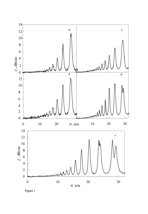
FIG. 1.: Absorption coefficient $\Gamma$ versus magnetic field $H$ at frequency $f$=30 MHz at temperatures T,K: a-4.2, b-3.8, c-e-1.5 and wave power at the oscillator output $P$, W: a-c-$10^{-5}$, d-$10^{-4}$ e-$10^{-3}$.

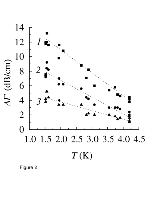
FIG. 2.: $\Delta\Gamma=\Gamma_{max}-\Gamma_{min}$ versus temperature $T$ in the linear regime at a frequency of 150 MHz in a magnetic field $H$, kOe: $1$-17.5, $2$-15.5, $3$-14.1.

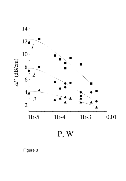
FIG. 3.: $\Delta\Gamma=\Gamma_{max}-\Gamma_{min}$ versus the power $P$ at the oscillator output in the linear regime at a frequency of 150 MHz in a magnetic field $H$, kOe: 1-17.5,2-15.5, 3-14.1.

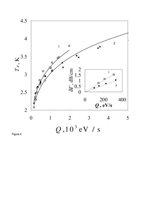
FIG. 4.: Electron temperature $T_{e}$ versus the energy losses $Q$ at SAW frequencies $f$, MHz: $1$-150 and $2$-30. Inset: $\delta\Gamma=\Gamma(T_{e})-\Gamma_{0}(T)$ versus $Q$ at SAW frequencies $f$ MHz: $1$-150, $2$-30.

REFERENCES

- [1] Yu. M. Gal’perin, I. L. Drichko, and B. D. Laikhtman, Fiz. Tverd. Tela (Leningrad) 12, 1437 (1970) [Sov. Phys. Solid Stale 12, 1128 (1970)].
- [2] I. L. Drichko, Fiz. Tverd. Tela (Leningrad) 27, 499 (1985) [Sov. Phys. Solid State 27, 305 (1985)].
- [3] Yu. M. Gal’perin, I. L. Drichko, and L. B. Litvak-Gorskaya, Fiz. Tverd. Tela (Leningrad) 28, 3374 (1986) [Sov. Phys. Solid Stale 28, 1899 (1986)].
- [4] Yu. M. Gal’perin, I. L. Drichko, and L. B. Litvak-Gorskaya in Proceedings of a Conference on Plasma and Instabililies in Semiconduciors [in Russian], Vil’nyus, 1986. p. 186.
- [5] A. Wixforth. J. Scriba, M. Wassermeier, J. P. Kotthaus, G. Weimann, and W. Schlapp, Phys. Rev. B 40, 7874 (1989).
- [6] A. Schenström, M. Levy, B. K. Sarma, and H. Morkoč, Solid State Com-mun. 68,357 (1988).
- [7] I. L. Drichko, A. M. D’yakonov, A. M. Kreshchuk, T. A. Polyanskaya, I. G. Savel’ev, I. Yu. Smirnov. and A. V. Suslov, Fiz. Tekh. Poluprovodn. 31, 451 (1997) [Semiconductors 31, 384 (1997)].
- [8] M. G. Blyumina. A. G. Denisov, T. A. Polyanskaya, I. G. Savel’ev, A. P. Senichkin, and Yu. V. Shmartsev, Fiz. Tekh. Poluprovodn. 19. 164 (1985) [Sov. Phys. Semicond. 19, 102 (1985)].
- [9] I. L. Drichko and I. Yu. Smirnov. Fiz. Tekh. Poluprovodn. 31. 1092 (1997) [Semiconductors 31. 933 (1997)].
- [10] V. F. Gantmakher and I. B. Levinson, Current Carrier Scattering in Metals and Semiconductors [in Russian], Nauka, Moscow, 1984.
- [11] M. G. Blyumina, A. G. Denisov, T. A. Polyanskaya, I. G. Savel’ev, A. P. Senichkin, and Yu. V. Shmartsev, JETP Leu. 44. 331 (1986).
- [12] I. G. Savel’ev, T. A. Polyanskaya, and Yu. V. Shmartsev, Fiz. Tekh. Poluprovodn. 21, 2096 (1987) [Sov. Phys. Semicond. 21, 1271 (1987)].
- [13] A. M. Kreshchuk, M. Yu. Martisov. T. A. Polyanskaya, I. G. Savel’ev, I. I. Saidashev. A. Yu. Shik, and Yu. V. Shmartsev, Fiz. Tekh. Poluprovodn. 22, 604 (1988) [Sov. Phys. Semicond. 22. 377 (1988)].
- [14] A. M. Kreshchuk, M. Yu. Martisov, T. A. Polyanskaya, I. G. Savel’ev, I. I. Saldashev, A. Yu. Shik, and Yu. V. Shmartsev, Solid State Commun. 65,1189(1988).
- [15] A. M. Kreshchuk, E. P. Laurs. T. A. Polyanskaya, I. G. Savel’ev, I. I. Saidashev, and E. M. Semashko, Fiz. Tekh. Poluprovodn. 22,2162(1988) [Sov. Phys. Semicond. 22, 1364 (1988)].
- [16] V. Karpus, Fiz. Tekh. Poluprovodn. 22, 439 (1988) [Sov. Phys. Semicond. 22,268 (1988¿].
- [17] V. Karpus, Fiz. Tekh. Poluprovodn. 20. 12 (1986) [Sov. Phys. Semicond. 20,6(1986)].
- [18] A. V. Chaplik, Zh. Eksp. Teor. Fiz. 60, 1845 (1971) [Sov. Phys. JETP 33, 997 (1971)].
- [19] H. Fukuyama and E. Abrahams. Phys. Rev. B 27, 5976 (1983).
- [20] B. L. Al’tshuler and A. G. Aronov, JETP 30, 482 (1979).
- [21] F. Schmid, Z. Phys. 217, 251 (1979).
- [22] B. L. Altshuler, A. G. Aronov, and D. E. Khmelnitskii, J. Phys.: Condens. Matter 15,73 (1982).
- [23] I. G. Savel’ev and T. A. Polyanskaya, Fiz. Tekh. Poluprovodn. 22, 1818 (1988) [Sov. Phys. Semicond. 22, 1150 (1988)].
- [24] A. R. Hutson and D. L. White. J. Appl. Phys. 33, 40 (1962).