Magneto-shear modes and a.c. dissipation in a two-dimensional Wigner crystal

Abstract

The a.c. response of an unpinned and finite 2D Wigner crystal to electric fields at an angular frequency $\omega$ has been calculated in the dissipative limit, $\omega\tau\ll 1$, where $\tau^{-1}$ is the scattering rate. For electrons screened by parallel electrodes, in zero magnetic field the long-wavelength excitations are a diffusive longitudinal transmission line mode and a diffusive shear mode. A magnetic field couples these modes together to form two new magneto-shear modes. The dimensionless coupling parameter $\beta=2(c_{t}/c_{l})|\sigma_{xy}/\sigma_{xx}|$ where $c_{t}$  and $c_{l}$ are the speeds of transverse and longitudinal sound in the collisionless limit and $\sigma_{xy}$ and $\sigma_{xx}$ are the tensor components of the magnetoconductivity. For $\beta\geqslant 1$, both the coupled modes contribute to the response of 2D electrons in a Corbino disk measurement of magnetoconductivity. For $\beta\gg 1$, the electron crystal rotates rigidly in a magnetic field. In general, both the amplitude and phase of the measured a.c. currents are changed by the shear modulus. In principle, both the magnetoconductivity and the shear modulus can be measured simultaneously.

]

I Introduction

Free electrons deposited above the surface of liquid helium form a two-dimensional (2D) conducting system which has been intensively studied in recent years [1]. The typical surface concentrations, $n<2\times 10^{9}\;{\rm cm}^{-2}$, for electrons on helium are small compared to those in semiconductor heterostructures and provide complementary information about the phases and kinetic properties of strongly interacting 2D electron systems. It was established long ago [2, 3] that at very low temperatures ($T<1\;{\rm K}$) the electron system undergoes a transition from the liquid to the solid phase, where the electrons form a Wigner crystal (WC). More recently, there has been great interest in the kinetics of the WC in an applied magnetic field. Fascinating non-linear effects have been discovered regarding the WC magnetoconductivity, including magnetoconductivity hysteresis [4] and Bragg-Cherenkov scattering [5, 6].

A specific feature of the 2D electrons on helium is the inability to make direct ohmic contacts to the electron layer. The kinetic coefficients of 2D electrons are studied using capacitative coupling between the electrons and an array of electrodes. The electrons can be held in place above the helium surface by a positive d.c. voltage applied to the electrodes below the helium surface. The kinetics of the electron system are studied by applying a small a.c. voltage, angular frequency $\omega$, to one or more electrodes and by measuring the a.c. current flow to other electrodes. Due to the capacitative coupling between the electrodes and the electron sheet, the electron system behaves as a transmission line, and its kinetic coefficients define the magnitude and phase of the a.c. currents with respect to the applied voltage. The connection between the phase shift and the conductivity is known for the electron liquid [7]. In the case when the electrons form a crystal, however, an additional study is needed because of the shear modulus, which exists for the electron solid but is absent in the liquid phase, though the kinematic viscosity may be significant in a highly correlated liquid.

The goal of this paper is to present such a study and to show the connection between the microscopic kinetic coefficients of the WC and its macroscopic a.c. response as observed experimentally. We are not considering the mechanism of conductivity in unpinned WC [8, 9], and the microscopic long-wavelength magnetoconductivity is a parameter in our theory. It should be noted that the kinetic properties of the WC and the electron liquid are, in the general case, substantially different. In particular, the conductivity of the WC on ${}^{\text{4}}$He is strongly nonlinear in zero and moderate applied magnetic fields [4, 5] due to the Bragg-Cherenkov mechanism of energy losses [6]. Strong magnetic fields, however, smear out the Bragg-Cherenkov resonances and the conductivity of the WC becomes linear and is the same as in the liquid phase. [10] Only this case, when the WC kinetics can be described by linear and local conductivity, will be considered in this paper. However the shear rigidity of the crystal means that the total response of a finite size WC to an applied force will be non-local and must be calculated explicitly for each electrode geometry.

The conductivity of the Wigner solid on normal and superfluid ${}^{\text{3}}$He has recently been measured by Shirahama et al. [11] and a linear conduction region is observed, in contrast to the non-linear effects on ${}^{\text{4}}$He. The theory given here should therefore apply to the Wigner solid on ${}^{\text{3}}$He in all magnetic fields.

The analysis can be simplified using several limiting conditions. First we assume that the 2D electrons are in the ”screened limit”, with the wavelength of the excitations $\lambda\gg d$, the electron-electrode separation, which acts as a screening length. Secondly, the low frequencies used experimentally (typically in the audio frequency range) are in the dissipative limit with $\omega\tau\ll 1$, where $\tau^{-1}$ is a scattering rate. We show below that for a Wigner crystal there exist two important low-frequency bulk magnetoplasmon modes. In the case of a small shear modulus and/or a small applied magnetic field, one of these modes is similar to the dissipative longitudinal magnetoplasmons in the electron liquid [7], while the other is connected to a pure shear diffusive mode. A perpendicular magnetic field mixes these modes, as it does the two phonon branches of the WC [12, 13]. The mixing parameter behaves as $\mu\left|\sigma_{xy}/\sigma_{xx}\right|$, where $\mu$ is the shear modulus, $\sigma_{xx}$ and $\sigma_{xy}$ are diagonal and off-diagonal components of the conductivity tensor. The mixing becomes large in classically strong magnetic fields, when $\left|\sigma_{xy}/\sigma_{xx}\right|\gg 1$, and both modes, which we will refer as magneto-shear modes, should be taken into account. We then analyze the a.c. response of the Wigner crystal for the Corbino geometry of electrodes, as used for magnetoconductivity measurements [4, 5, 14].

The coupling of the longitudinal and transverse modes in the collisionless limit, $\omega\tau>>1$, has been analysed and used experimentally to obtain the shear modulus of the WC by Deville et al.[15]. The dynamical matrix for 2D electrons on helium in a magnetic field, including the coupling to the surface ripplons, was given by Shikin and Williams [16]. An analysis of the shear mode resonances of 2D charged ions [17] below the surface of liquid helium in a magnetic field has been given by Appleyard et al. [18]. This system is formally identical to the one studied here, though the parameter ranges are quite different, and we concentrate here on the dissipative and screened limit.

The paper is organized in the following way. In Section II we study the magneto-shear modes of a 2D Wigner solid in an applied magnetic field. In Section III we present the theory of the a.c. response of the Wigner solid in the Corbino geometry. Finally, Section IV contains the discussion of the results, and conclusions.

II Magneto-shear modes

Let the electrons of the WC experience a displacement ${\bf u}({\bf r})$, where ${\bf r}=(x,y)$ is the 2D coordinate in the plane of the crystal. The electric field ${\bf E(r)}$ arising in this plane can be written as a sum of two terms, ${\bf E(r)=E}_{c}({\bf r})+{\bf E}_{s}({\bf r})$. The first term, ${\bf E}_{c}({\bf r})$, appears due to the change in the electric-charge density, $\delta\rho({\bf r)}=en{\bf\nabla}\cdot{\bf u}({\bf r})$ ($n$ is the concentration of electrons), and is the same as for a normal electron fluid. The second term is specific for the electron solid and exists due to the shear deformation:

$${\bf E}_{s}({\bf r})=\frac{\mu}{ne}{\bf\nabla}\times\left({\bf\nabla}\times{\bf u}({\bf r})\right).$$ (1)

If the displacement field is smooth over the distance between the electron sheet and the electrodes $d$ (typical wave-length $\lambda\gg d$, the screened limit), one can use the local relation between the change in the electron density $\delta\rho({\bf r})$ and the electric field ${\bf E}_{c}({\bf r})$. In this case the main change in the electric potential $\delta V({\bf r})$ is attributed to the image forces in the electrodes, $\delta V({\bf r})=\delta\rho({\bf r})/C_{s}$, and

$${\bf E}_{c}({\bf r})=-\frac{ne}{C_{s}}{\bf\nabla}\left({\bf\nabla}\cdot{\bf u(r)}\right),$$ (2)

where $C_{s}$ is the capacitance per unit area (for the electrons on helium $C_{s}$ is equal to $\varepsilon_{{\rm He}}/(4\pi d)$, with $\varepsilon_{{\rm He}}$ being the dielectric permittivity of the liquid helium) [19].

In what follows we consider harmonic excitation of the WC, when all relevant quantities change with time as $\exp(i\omega t)$ (we will not write down this time dependence explicitly). We assume, as was discussed in Section I, that the Wigner crystal in the magnetic field $B$ applied perpendicular to the electron layer exhibits linear and local conductivity given by a conductivity tensor ${\bf\sigma}\left(\omega\right)$. Than one can find from Eqs.(1),(2) that the density of electric current ${\bf j(r)}=-i\omega ne{\bf u(r)}$ for the excitations of the WC satisfies the equation

$$i\omega C_{s}{\bf j}({\bf r})={\bf\sigma}(\omega)\cdot\left[{\bf\nabla}\left({\bf\nabla}\cdot{\bf j}({\bf r})\right)-\gamma{\bf\nabla}\times\left({\bf\nabla}\times{\bf j}({\bf r})\right)\right],$$ (3)

where

$$\gamma=\mu C_{s}/(ne)^{2}.$$ (4)

Before considering the dissipative magnetoplasmons we note that Eq.(3) also describes the excitations of the WC in the collisionless limit. In particular, in the zero-field case ($B=0$), when the components of the conductivity tensor are $\sigma_{xx}(\omega)=\sigma_{yy}(\omega)=ne^{2}/(i\omega m)$ and $\sigma_{xy}(\omega)=\sigma_{yx}(\omega)=0$ ($m$ is the electron mass), it gives the two phonon branches of the crystal. In the screened limit these long-wavelength excitations are acoustic in nature. The velocities of the longitudinal and transverse sound waves are $c_{l}=\left(ne^{2}/mC_{s}\right)^{1/2}$ and $c_{t}=(\mu/mn)^{1/2}$, so that the dimensionless parameter $\gamma$ entering Eq.(3) is just their squared ratio, $\gamma=(c_{t}/c_{l})^{2}$.

In the dissipative and screened limit, the longitudinal plasma mode, without shear, has a wavevector $k$ [20]

$$k^{2}=-\frac{i\omega C_{s}}{\sigma_{xx}}.$$ (5)

This diffusive mode is equivalent to a one-dimensional transmission line mode with distributed capacitance and resistance[21] as in a coaxial cable at low frequencies, for instance. This is the only relevant mode in the analysis of the Corbino geometry for a homogeneous, screened 2D electron fluid [7], with $\mu=0$, and in the WC in zero magnetic field. In the same limit, $\omega\tau<<1$, in zero field, the shear mode is also diffusive with a wavevector $q_{s}$

$$q_{s}^{2}=-\frac{i\omega mn}{\mu\tau}=-\frac{i\omega n^{2}e^{2}}{\mu\sigma_{xx}}\;$$ (6)

but this mode is not excited by the purely radial forces in zero magnetic field in the Corbino geometry.

We will analyze the dissipative magnetoplasmons using cylindrical in-plane polar coordinates ${\bf r}\equiv(r,\varphi)$, and we will be interested in the axisymmetric solutions of Eq.(3) where the current density does not depend on the angle $\varphi$. In this case, in terms of the radial $j_{r}(r)$ and angular $j_{\phi}(r)$ components of ${\bf j}(r)$, Eq.(3) gives

$$i\omega C_{s}j_{r}(r) = {\hat{D}}\left[\sigma_{xx}j_{r}(r)+\gamma\sigma_{xy}j_{\phi}(r)\right],$$ (8)

$$i\omega C_{s}j_{\phi}(r) = {\hat{D}}\left[-\sigma_{xy}j_{r}(r)+\gamma\sigma_{xx}j_{\phi}(r)\right],$$ (9)

using the diagonal $\sigma_{xx}=\sigma_{yy}$ and off-diagonal $\sigma_{xy}=-\sigma_{yx}$ components of the conductivity tensor in a magnetic field.

The operator ${\hat{D}}$,

$${\hat{D}=}\frac{d^{2}}{dr^{2}}+\frac{d}{rdr}-\frac{1}{r^{2}}\;,$$ (10)

in Eqs.(II) is the same as in the Bessel equation, and the solutions of Eqs.(II) are appropriate superpositions of the first order Bessel and Neumann functions, $J_{1}(qr)$ and $Y_{1}(qr)$. The allowed values of the wavevector $q$ can be found by substituting $j_{r}(r)=AJ_{1}(qr)$ and $j_{\phi}(r)=BJ_{1}(qr)$, which gives the linear equations

$$\left(i\omega C_{s}+\sigma_{xx}q^{2}\right)A+\gamma\sigma_{xy}q^{2}B = 0,$$ (12)

$$\sigma_{xy}q^{2}A-\left(i\omega C_{s}+\gamma\sigma_{xx}q^{2}\right)B = 0,$$ (13)

for the coefficients $A$ and $B$. It follows from Eqs.(10) that there are two magnetoplasmon or magneto-shear wavevectors, $q_{+}$ and $q_{-}$, such that

$$q_{\pm}^{2}=\frac{2k^{2}}{1+\gamma\pm\alpha},$$ (14)

and the relation between the coefficients is

$$B^{(\pm)}=-\frac{2}{\sqrt{\alpha^{2}+\beta^{2}}\pm\alpha}\frac{\sigma_{xy}}{\sigma_{xx}}A^{(\pm)}.$$ (15)

In Eqs. (14) and (15) we denoted

$$\beta^{2}=4\gamma\frac{\sigma_{xy}^{2}}{\sigma_{xx}^{2}}\;,\;\;\;\;\;\alpha=\sqrt{(1-\gamma)^{2}-\beta^{2}}.$$ (16)

The parameter $\gamma=\left(c_{t}/c_{l}\right)^{2}$ is small in many experiments on magnetoconductivity of electrons on helium. Using the expression for the transverse sound velocity in the WC $c_{t}\simeq 0.5(e^{2}n^{1/2}/m)^{1/2}$ [12], we find $\gamma\simeq 2\times 10^{-4}$ for typical electron concentrations $n\sim 10^{8}\;{\rm cm}^{-2}$ and an electron-electrode spacing $d\sim 10^{-2}\;{\rm cm}$. Eqs. (14) and (16) show that the mixing of the longitudinal and transverse dissipative magnetoplasmons is governed by the dimensionless parameter $\beta=2(c_{t}/c_{l})|\sigma_{xy}/\sigma_{xx}|$. The ratio $\sigma_{xy}/\sigma_{xx}$ can be large in classically strong magnetic fields, so that $\beta$ can become comparable to 1. In this case the magneto-shear mode wavevectors $q_{+}$ and $q_{-}$ (14) are of the same order of magnitude, both different from the wavevectors $k$, Eq.(5), and $q_{s}$, Eq.(6). Both magneto-shear modes are excited in the Corbino geometry and should be taken into account. The dependences of the magnetoplasmon wavevectors $q_{\pm}$ on $\beta^{2}$ are shown in Fig.1. In the $\beta\gg 1$ limit the wavevectors become

$$q_{-}=\sqrt{\frac{\omega\omega_{c}}{c_{t}c_{l}}}\;,\;\;\;\;\;\;\;\;\;\;q_{+}=-i\sqrt{\frac{\omega\omega_{c}}{c_{t}c_{l}}}\;,$$ (17)

corresponding to propagating and exponentially damped modes. In Eq.(17) we assumed that the Hall effect is given by the classical relation $\sigma_{xy}=nec/B$ and $\omega_{c}$ is the cyclotron frequency.

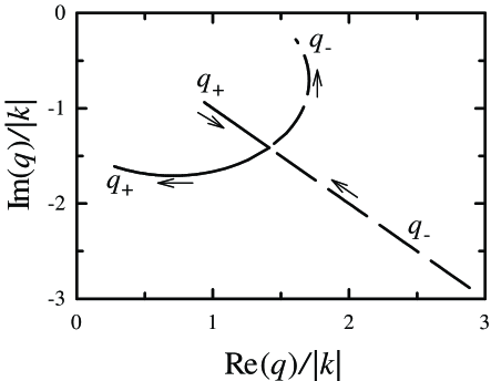
FIG. 1.: The change of the magnetoplasmon wavevectors $q_{+}$ (solid line) and $q_{-}$ (dashed line) given by Eq.(14) with increasing mixing parameter $\beta^{2}$, Eq.(16), as indicated by arrows. The wavevectors are presented in units of $\left|k\right|=\left|\omega C_{s}/\sigma_{xx}\right|^{1/2}$.

III Response of the Wigner crystal in the Corbino geometry

In this Section we calculate the spatial distribution of the electric current density in the Corbino geometry used in Ref.[14, 5]. The array of electrodes (Fig.2) consists of a central, driven, electrode $A$ with radius $r_{1}$ surrounded by a ring electrode $E$, which in turn is surrounded by outer, receiving, electrodes $B_{1}$, $B_{2}$, and $B_{3}$. Usually the spacing between the $B_{1,2,3}$ electrodes is made to be small, so that one can regard them as one ring electrode $B$. We denote the outer radius of the $B$ electrode as $r_{2}$, and the inner radius (which is approximately the same as the outer radius of the $E$ electrode) as $r_{3}$. Along with a constant voltage applied to the all electrodes, a small a.c. voltage $V_{0}\exp(i\omega t)$ is applied to the $A$ electrode. In the case when the sizes of the electrodes are much greater than the electron-electrode separation, $r_{1,2,3}\gg d$, it produces an electric field ${\cal E}=({\bf r}/r)V_{0}\delta(r-r_{1})\exp(i\omega t)$ in the plane of the WC. The induced electric currents can then be found as the solutions of Eq.(3) with

$$i\omega C_{s}V_{0}\delta(r-r_{1}){\bf\sigma}(\omega)\cdot\frac{{\bf r}}{r}$$ (18)

added to its right-hand side.

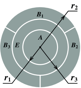
FIG. 2.: The Corbino electrodes geometry. Shown are the driven central electrode $A$ with radius $r_{1}$, the ring electrode $E$, and the receiving electrodes $B_{1,2,3}$. Three receiving elecrodes are needed experimentally to level the system and, since the spacings between them are small, they can be regarded as one ring electrode with inner radius $r_{3}$ and outer radius $r_{2}$.

According to the analysis in Section II, the radial $j_{r}(r)$ and angular $j_{\phi}(r)$ components of the density of electric current are appropriate superpositions of the cylindrical functions. Since the solutions cannot be singular at $r=0$, in the region $r<r_{1}$ we have

$$j_{r}(r) \equiv j_{r}^{<}(r)=A_{1}^{(+)}J_{1}(rq_{+})+A_{1}^{(-)}J_{1}(rq_{-}),$$ (20)

$$j_{\phi}(r) \equiv j_{\phi}^{<}(r)=B_{1}^{(+)}J_{1}(rq_{+})+B_{1}^{(-)}J_{1}(rq_{-}),$$ (21)

while for $r>r_{1}$ both Bessel and Neumann functions are present

$$j_{r}(r) \equiv j_{r}^{>}(r)=A_{2}^{(+)}J_{1}(rq_{+})+A_{2}^{(-)}J_{1}(rq_{-})$$ (24)

$$+A_{3}^{(+)}Y_{1}(rq_{+})+A_{3}^{(-)}Y_{1}(rq_{-}),$$

$$j_{\phi}(r) \equiv j_{\phi}^{>}(r)=B_{2}^{(+)}J_{1}(rq_{+})+B_{2}^{(-)}J_{1}(rq_{-})$$ (26)

$$+B_{3}^{(+)}Y_{1}(rq_{+})+B_{3}^{(-)}Y_{1}(rq_{-}).$$

The driving term (18) produces a jump in the derivative of $j_{r}(r)$ at the outer radius of the $A$ electrode, so that we have

$$j_{r}^{<}(r_{1}) = j_{r}^{>}(r_{1})\;,\;\frac{d}{dr}\left(j_{r}^{<}-j_{r}^{>}\right)_{r=r_{1}}=i\omega C_{s}V_{0};$$ (28)

$$j_{\phi}^{<}(r_{1}) = j_{\phi}^{>}(r_{1})\;,\;\frac{d}{dr}\left(j_{\phi}^{<}-j_{\phi}^{>}\right)_{r=r_{1}}=0.$$ (29)

The currents are also subject to the following conditions at the outer boundary of the WC (“stress-free boundary”):

$$j_{r}^{>}(r_{2})=0\;,\;\frac{d}{dr}\left(\frac{j_{\phi}^{>}}{r}\right)_{r=r_{2}}=0.$$ (30)

Substituting Eqs.(2),(III) into (2) and making use of the relations (15) between $A_{i}^{(\pm)}$ and $B_{i}^{(\pm)}$ $(i=1,2,3)$, one can find

$$A_{3}^{(\pm)}=\mp\frac{i\pi}{2}\left(\frac{\sqrt{\alpha^{2}+\beta^{2}}\pm\alpha}{2\alpha}\right)\omega r_{1}C_{s}V_{0}J_{1}(r_{1}q_{\pm}).$$ (31)

The coefficients $A_{2}^{(\pm)}$ can then be found from Eqs.(30), and $A_{1}^{(\pm)}$ from the continuity of currents at $r=r_{1}$. However, the final expressions are rather cumbersome, and we will present here some numerical results.

It turns out that the radial current density $j_{r}(r)$ does not exhibit strong qualitative changes as the mixing parameter $\beta$ (16) increases, and is similar to the case of the normal electron fluid where, for pure capacitative coupling with no losses

$$j_{r}\left(r\right) = i\omega C_{s}V_{0}\frac{\left(r_{2}^{2}-r_{1}^{2}\right)r}{2r_{2}^{2}},\hskip 21.68121ptr\leq r_{1}$$ (33)

$$j_{r}\left(r\right) = i\omega C_{s}V_{0}\frac{r_{1}^{2}\left(r_{2}^{2}-r^{2}\right)}{2r_{2}^{2}r},\hskip 21.68121ptr_{1}<r\leq r_{2}.$$ (34)

It increases (approximately linearly) in the region $r<r_{1}$, and then decreases monotonously for $r>r_{1}$, going to zero at $r=r_{2}$. More drastic changes, however, happen to the angular component of the density of current $j_{\phi}(r)$, as is illustrated in Fig.3. We note that, in the case of a normal electron fluid ($\gamma=0$), the angular and radial components of the density of current are proportional, $j_{\phi}(r)=-(\sigma_{xy}/\sigma_{xx})j_{r}(r)$ (also seen from Eqs.(II)). This relation remains approximately true for the WC in a weak applied magnetic field, when both $\gamma$ and $\beta$ are small. The angular density of current then follows the dependence $j_{r}(r)$ with a cusp at the outer boundary of the driven electrode $A$ ($r=r_{1}$). This limiting case is shown by the thin solid line in Fig.3. Increasing the applied magnetic field and hence the mixing parameter $\beta$ makes the $j_{\phi}(r)$ dependence much smoother. In the region of classically strong magnetic fields, when $\left|\sigma_{xy}/\sigma_{xx}\right|\gg 1$ and $\beta\sim 1$, the angular current density increases linearly with radius (thin dashed line in Fig.3), which corresponds to the rigid rotation of the Wigner crystal as a whole in an applied magnetic field. It can be shown that in the rigid limit, $\beta\gg 1$, the angular density of current is

$$j_{\phi}(r)=\frac{1}{2}\left(1-\frac{r_{1}^{2}}{r_{2}^{2}}\right)\frac{(kr_{1})^{2}}{1-\frac{1}{24}(kr_{2})^{2}}\frac{\sigma_{xy}V_{0}}{r_{2}^{2}}r\;.$$ (35)

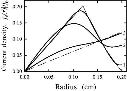
FIG. 3.: The radial dependence of the absolute value of the angular current density $|j_{\phi}(r)|$ for the mixing parameter $\beta^{2}=$ 0.01, 0.1, and 0.5 (curves 1, 2, and 3). The asymptotic dependences for $\beta\rightarrow 0$ (thin solid line) and $\beta\rightarrow\infty$ (thin dashed line) are shown. The calculations were carried out for $\left|kr_{2}\right|=1$, $r_{1}=0.6r_{2}$, and $r_{2}=0.2\;{\rm cm}$. The density of current is given in units of $j_{0}=(\pi/2)\left|\sigma_{xy}/\sigma_{xx}\right|\omega r_{1}C_{s}V_{0}$.

For the Corbino electrodes shown in Fig.2, the experimentally measured a.c. current $I$ is collected by the $B$ electrode,

$$I=2\pi r_{3}j_{r}(r_{3})$$ (36)

assuming that all current which flows through the inner radius $r_{3}$ is collected. It can be shown that the phase shift between the current $I$ and the driving voltage $V_{0}$ is $\pi/2$ as $\left|k\right|\rightarrow 0$ (i.e. $\left|\sigma_{xx}\right|\rightarrow\infty$, see Eq.(5)), so that $I=iI_{0}$ in this limit. The amplitude $I_{0}$ is the same both with and without a finite shear modulus,

$$I_{0}=\pi\frac{r_{1}^{2}}{r_{2}^{2}}\left(r_{2}^{2}-r_{3}^{2}\right)\omega C_{s}V_{0}\;.$$ (37)

For a finite value of $\sigma_{xx}$ the measured current acquires a real component, in phase with $V_{0}$, and it is convenient to illustrate the effects of the mixing of the two magneto-shear modes using an Argand diagram to show the current in the complex $I$-plane. Such Argand diagrams are shown in Fig.4.

IV Discussion and Conclusions

We have calculated the response of a 2D charged crystal to the low frequency excitation of a Corbino disk in the screened, dissipative limit. In zero magnetic field, the electrical response is the same as for a homogeneous 2D electron fluid, and depends only on the wavevector $k$ of the transmission line mode. This assumes that the crystal is not pinned (note that this is in contrast to the WC in semiconductors) and that no dislocations are generated by the local electron density gradients, which could give rise to extra losses. For no losses, the measured current is purely capacitative. For a finite conductivity, the complex current follows a distinctive locus on an Argand diagram (curve 1 in Fig.4) as $\sigma_{xx}$ and hence $|k|$ changes. The phase shift away from pure capacitative coupling, $\theta\propto 1/\sigma_{xx}$ for small phase shifts.

For a 2D fluid in a magnetic field, the same result is obtained. An azimuthal Hall current flows $j_{\phi}(r)=-(\sigma_{xy}/\sigma_{xx})j_{r}(r)\approx-\omega_{c}\tau$ $j_{r}(r)$ but is not detected. The Lorentz force on the electrons is balanced locally by the a dissipative drag force $F_{d}(r)\varpropto-v_{H}(r)\varpropto-j_{\phi}(r)$ in classically strong fields, where $v_{H}(r)$ is the Hall velocity of the electrons. The measured phase shift $\theta\propto 1/\sigma_{xx}(B)$.

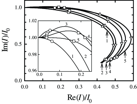
FIG. 4.: The Argand diagram locus for the measured radial current $I$ (see text) with increasing shear parameter: $\beta^{2}=$ 0, 0.1, 0.5, 0.99, and 2.0 (curves 1, 2, 3, 4, and 5), calculated for wavevector $\left|k\right|=\left|\omega C_{s}/\sigma_{xx}\right|^{1/2}$ values from 1 to 30 cm^-1. For five values of $\left|k\right|$ we have indicated by symbols the actual positions of the complex vector representing the radial current: $\left|k\right|$ = 5 cm^-1 ($\bigcirc$), 10 cm^-1 ($\square$), 15 cm^-1 ($\triangle$), 20 cm^-1 ($\nabla$) and 25 cm^-1 ($\Diamond$). The upper part of the Argand diagram is shown in enlarged form in the inset. The components of the current are given in units of $I_{0},$ Eq.(37). The geometry of the Corbino electrodes was $r_{1}=0.12$ cm, $r_{2}=0.2$ cm, and $r_{3}=0.14$ cm, corresponding to Ref.[5, 14].

In the WC, the shear modulus gives rigidity. In a magnetic field in the rigid limit, the crystal can only rotate uniformly with $j_{\phi}(r)\varpropto r$. The Lorentz forces on the capacitative radial currents produce a torque which is balanced by the torque from the local drag forces $F_{d}(r)\varpropto-j_{\phi}(r)$. In this limit, the measured phase shift $\theta$ is reduced by a factor $0.54$ as compared to fluid rotation with the same drag coefficient. The losses, as expressed in the phase shift, depend on the azimuthal current distribution. Thus the effective Corbino magnetoconductivity increases by a factor $1.87$ (for small phase shifts) if the crystal starts to rotate rigidly. At the same time the magnitude of the current changes and the measured current leaves the normal locus for a 2D conducting fluid on the Argand diagram, as shown in Fig.4.

In general, the response will lie between the fluid and rigid limits, controlled by the dimensionless parameter $\beta=2(c_{t}/c_{l})|\sigma_{xy}/\sigma_{xx}|$ and the propagation of the two magneto-shear modes. Note that $\beta$ increases as the helium depth $d$ decreases. The azimuthal current density distribution depends on the value of $\beta$, being linear in $r$ near the origin and also at the circumference of the Corbino disc, due to the stress free boundary condition, as shown in Fig.3. The loci of the measured current $I$, as the conductivity decreases (giving values of $|k|=|\omega C_{s}/\sigma_{xx}|^{1/2}$ from 1 to 30 cm${}^{\text{-1}}$), for fixed values of $\beta^{2}=$ $0$ (fluid), $0.1,$ $0.5,0.99$ and $2.0$ are shown in Fig.4. This behavior is a key indication of shear rigidity. For five values of $\left|k\right|$ we have indicated by symbols the actual positions of the complex vector representing the radial current: $\left|k\right|$ = 5 cm^-1 ($\bigcirc$), 10 cm^-1 ($\square$), 15 cm^-1 ($\triangle$), 20 cm^-1 ($\nabla$) and 25 cm^-1 ($\Diamond$) for the different values of $\beta$. These points indicate the change in the current as the shear parameter increases for a given conductivity. In principle, the measurement of both components of the complex a.c. current $I$ should enable both the magnetoconductivity $\sigma_{xx}$ and the shear modulus $\mu$ to be determined, assuming that the Hall effect is given by the classical result, $\sigma_{xy}=nec/B$, in all cases.

Experimentally, three regions can be approximated in the field dependence of the magnetoconductivity $\sigma_{xx}$ and hence $\beta$. In low fields in the fluid phase [22], the Drude model holds with $\sigma_{xx}=\sigma_{0}/(1+\omega_{c}^{2}\tau^{2})$ with a scattering time $\tau$ which is independent of magnetic field, due to many-electron effects [23]. The Drude model also holds in the WC above liquid ${}^{\text{3}}$He [11]. This would give $\beta\varpropto B$. But for the WC on liquid ${}^{\text{4}}$He, the magnetoconductivity in low fields is non-linear with $\sigma_{xx}\varpropto 1/B$ with a proportionality constant which depends on the drive voltage. This would give $\beta$ independent of field, though the shear-mode theory given here only applies to a linear response. Above 1 Tesla, the magnetoconductivity in the WC is much less field dependent [10], and is almost independent of drive voltage. A constant $\sigma_{xx}$ gives $\beta\varpropto 1/B$. Hence experimentally $\beta$ should increase with magnetic field, pass through a maximum and decrease again at higher fields. An analysis of recent experimental data in the WC will be given elsewhere.

In conclusion, we have shown that strong enough applied magnetic field mixes the diffusive longitudinal plasma and shear modes of 2D Wigner crystal, forming two diffusive magneto-shear modes. Both coupled modes contribute in the a.c. response of the Wigner crystal. This gives a crossover from the liquid-like response of the Wigner crystal at small values of the coupling parameter $\beta$ to rigid a.c. behavior in the strong coupling limit. Both the shear modulus and dissipative magnetoconductivity of the 2D Wigner crystal can, in principle, be measured simultaneously from the amplitude and phase of the a.c. response.

V Acknowledgments

We are grateful to Mark Dykman for illuminating discussions. One of us (Y.G.R.) wishes to thank Royal Holloway, University of London for the warm hospitality extended to him during his visit, when some of this work was done, partly supported by the Royal Society.

REFERENCES

- [1] 2D Electron Systems on Helium and Other Substrates, ed. by E.Y. Andrei (Kluwer Academic, New York 1997); for an introductory review on electrons on helium see A.J. Dahm and W.F. Vinen, Physics Today 40, 43 (1987).
- [2] C.C. Grimes and G. Adams, Phys. Rev. Lett. 42, 795 (1979).
- [3] D.S. Fisher, B.I. Halperin, and P.M. Platzman, Phys. Rev. Lett. 42, 798 (1979).
- [4] K. Shirahama and K. Kono, Phys. Rev. Lett. 74, 781 (1995); K. Kono and K. Shirahama, Surf. Sci. 361 - 362, 826 (1996); J. Low Temp. Phys. 104, 237 (1996).
- [5] A. Kristensen, K. Djerfi, P. Fozooni, M.J. Lea, P.J. Richardson, A. Santrich-Badal, A.Blackburn, R.W. van der Heijden, Phys. Rev. Lett. 77, 1350 (1996).
- [6] M.I. Dykman and Y.G. Rubo, Phys. Rev. Lett. 78, 4813 (1997).
- [7] R. Mehrotra and A.J. Dahm, J. Low Temp. Phys. 67, 115 (1987).
- [8] M.I.Dykman and L.S.Khazan, JETP 50, 747 (1979).
- [9] M.I.Dykman, J. Phys. C 15, 7397 (1982); JETP 55, 766 (1982).
- [10] M.I.Dykman and M.J.Lea, Physica (1998) in press.
- [11] K. Shirahama, O.I.Kirichek, and K. Kono, Phys. Rev. Lett. 79, 4218 (1997).
- [12] L. Bonsall and A.A. Maradudin, Phys. Rev. B 15, 1959 (1977).
- [13] H. Fukuyama, Solid State Comm. 19, 551 (1976); F.P.Ulinich and N.A.Usov, Sov. Phys. JETP 49, 147 (1979).
- [14] M.J.Lea, P.Fozooni, P.J.Richardson, and A.Blackburn, Phys. Rev. Lett. 73, 1142 (1994).
- [15] G.Deville, A.Valdes, E.Y.Andrei and F.I.B.Williams, Phys.Rev.Lett. 53, 588 (1984).
- [16] V.B.Shikin and F.I.B.Williams, J. Low Temp. Phys. 43, 1 (1981).
- [17] P.L.Elliott, A.A.Levchenko, C.I.Pakes, L.Skrbek, and W.F.Vinen, Surf. Sci. 362, 843 (1996); P.L.Elliott, C.I.Pakes, L.Skrbek and W.F.Vinen, Czech.J.Phys. 46, S1, 335 (1996); P.L.Elliott, S.S.Nazin, C.I.Pakes, L.Skrbek, W.F.Vinen, and G.F.Cox, Phys. Rev. B 56, 3447 (1997).
- [18] N.J.Appleyard, P.L.Elliott, C.I.Pakes, L.Skrbek and W.F.Vinen, J.Phys: Condens. Matter 7, 8939 (1995).
- [19] When not only the electrodes below the helium surface are present, but there is also a top-plate above the electrons, the expression for should be modified. The analysis of magnetoplasmons of arbitrary wave-length for normal electron fluid in this case, including retardation, is given in: A.M.Kosevich, Yu.A.Kosevich, and J.C.Granada, Sov. J. Low Temp. Phys. 14, 509 (1988) [Fiz. Nizk. Temp. 14, 926 (1988)].
- [20] L.D.Landau and E.M.Lifshitz, Electrodynamics of Continuous Media, Pergamon, London, 1960.
- [21] M.J.Lea, A.O.Stone, P.Fozooni and J.Frost, J. Low Temp. Phys. 85, 67 (1991).
- [22] M.J. Lea, P. Fozooni, A. Kristensen, P.J. Richardson, K. Djerfi, M.I. Dykman, C.Fang-Yen and A.Blackburn, Phys. Rev. B 55, 16280 (1997).
- [23] M.I.Dykman, C.Fang-Yen and M.J.Lea, Phys. Rev. B 55, 16249 (1997).