Polymer adsorption on heterogeneous surfaces

Abstract

The adsorption of a single ideal polymer chain on energetically heterogeneous and rough surfaces is investigated using a variational procedure introduced by Garel and Orland (Phys. Rev. B 55 (1997), 226). The mean polymer size is calculated perpendicular and parallel to the surface and is compared to the Gaussian conformation and to the results for polymers at flat and energetically homogeneous surfaces. The disorder-induced enhancement of adsorption is confirmed and is shown to be much more significant for a heterogeneous interaction strength than for spatial roughness. This difference also applies to the localization transition, where the polymer size becomes independent of the chain length. The localization criterion can be quantified, depending on an effective interaction strength and the length of the polymer chain.

I Introduction

The adsorption of polymers on flat and homogeneous attractive surfaces has been the subject of many investigations, see e.g. [1, 2], but naturally occurring surfaces usually are rough and/or energetically inhomogeneous, the heterogeneity leading to an enhancement of adsorption under quite general conditions [3, 4, 5, 6, 7, 8, 9, 10, 11]: already simple physical arguments contain the statement that upon increasing the surface irregularity, the number of polymer-surface interactions is strongly enhanced relative to the idealized planar surface (see figure 1). This is a consequence of a larger probability of polymer-surface intersection with increasing roughness.

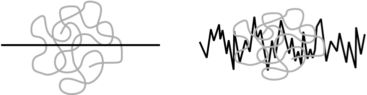
FIG. 1.: Sketch of the main mechanism of adsorption enhancement by surface roughness: the number of possible binding sites increases without being balanced by a loss in configurational entropy.

The study presented here is partly motivated by the theoretical investigation of reinforcement mechanisms in carbon black filled elastomers, where the polymer adsorption is substantial as there is a strong binding of the polymers to the surface (leading to a layer of localized polymers, the so called ”bound rubber” [12, 13]). These surfaces are rough and even fractal on many decades of their size, down to the molecular size range, as well as highly energetically (i.e. chemically) heterogeneous: the distribution of interaction strengths can be characterized by high energy sites surrounding a relatively low energy background. Therefore in principle both kinds of disorder should be incorporated in a theory which is supposed to explain the bound rubber phenomenon.

In the literature so far spatial and energetical heterogeneities were always treated separately. In this paper we want to present a treatment which covers both sorts of surface heterogeneity, thereby making possible a comparison concerning the strength of adsorption enhancement. Thus the general aim of the present paper is to produce a theory for the adsorption and localization of polymers on such surfaces. This is a nontrivial problem. For flat surfaces the description of ideal polymers by Schrödinger type equations is regarded as the method of choice, but for rough surfaces this method cannot be used in general, because the equations can be solved only for some highly specific boundary conditions, e.g., regular fractal surfaces [8]. Here we want to investigate the polymer behavior near surfaces with any type of surface disorder, as well as surfaces with a wide range of heterogeneities in the attractive potential. Therefore a path integral formalism seems to be appropriate, since the surface disorder can be dealt with explicitly up to an advanced stage of the calculation and disorder averages are less difficult.

However, some technical problems appear, forcing us to restrict the investigation to an idealized model system: a single ideal polymer chain in interaction with an attractive, penetrable, infinite surface. The treatment of real chains would require field theoretical approaches [1, 14] which are beyond the scope of the present paper. The penetrability of the surface (both sides of the surface are accessible for the polymer), which is of interest in the context of polymer chains at membranes or interfaces, here has to be assumed in order to avoid complex boundary conditions. In the problem of polymer adsorption on flat surfaces, non-penetrability is relatively easy to handle: the polymers are considered in half space [1, 2]. For random surfaces an half space treatment is no longer possible. Therefore we will loose information on the localization behavior, but nevertheless expect general insight into the problem.

The results of the calculations are expressions for the size of the chain, depending on the mean interaction strength $w_{0}$, the chain length $N$ and the disorder parameters. The paper is organized as follows. The size of the chain $R_{\bot}$ perpendicular to the surface is obtained

• in section II for strong spatial disorder, using a scaling argument à la de Gennes [19] – this calculation intends to give a better insight into the main mechanism of adsorption enhancement;

• in section III for weak spatial disorder and energetically heterogeneous surfaces, using a variational calculation.

In the latter case, first the Hamiltonian is formulated which explicitly contains the surface geometry and a distribution of interaction strengths. Then the free energy is approximated using a Feynman variational procedure. It turns out that for our problem an extension of a trial Hamiltonian introduced by Garel and Orland [15] is much more suitable than the replica trial Hamiltonian frequently used in connection with polymers in disordered environments [16, 17, 18]. In comparison with Garel and Orland, our main modification is the separation of the monomer coupling parameter into components of different space direction, thus enabling the polymer size parallel and perpendicular to the surface normal to be distinguished. After minimization of the free energy, the effect of surface heterogeneity can be summarized in an effective interaction strength which in most cases is larger than the mean interaction strength. The variational scheme is first tested on a flat and homogeneous surface, where it is shown that the result agrees with the scaling estimate and the results given earlier [1, 2] for ideal chains. Then the effective interaction strength is calculated for the special cases of a periodic and random distribution of interaction strength on a flat surface and for a periodic and random surface profile at constant interaction strength, respectively. This also allows us to consider the localization transition. The results are discussed and summarized in section IV.

II Scaling Argument for Fractal Spatial Disorder

A Flat Surface

First we briefly review a simple scaling treatment of an ideal chain adsorbed on a flat surface, as introduced by de Gennes [19]. Let $R_{\bot}$ and $R_{||}\simeq R_{0}\simeq bN^{1/2}$ be the mean size of an ideal polymer (with $N$ monomers and effective monomer length $b$) perpendicular and parallel to the surface, respectively. The monomer density is assumed to be constant in a region of size $R_{\bot}R_{||}^{2}$. Then the number $\cal N$ of monomers bounded to the surface is estimated as

$${\cal N}\ =\ bR_{||}^{2}\;{N\over R_{\bot}R_{||}^{2}}\ =\ {b\,N\over R_{\bot}}.$$ (1)

Consequently the free energy can be written as

$$\beta F\ \approx\ {R_{0}^{2}\over R_{\bot}^{2}}-\beta w\,{\cal N}\ =\ {b^{2}N\over R_{\bot}^{2}}-\beta w\;{bN\over R_{\bot}},$$ (2)

the first term being the confinement energy, the second one due to contact interactions with the surface ($-w$ is the effective monomer attraction, $\beta$ the inverse temperature). Minimization of the free energy ${\partial F/\partial R_{\bot}}=0$ gives an expression for the polymer thickness $R_{\bot}$ perpendicular to the surface,

$$R_{\bot}\simeq{b\over\beta w}.$$ (3)

Thus the thickness of the polymer reduces with growing attractive interaction strength, as expected. The independence of the chain length $N$ indicates that the polymer is in the so called ”localized” regime [18].

B Generalization for Fractal Surfaces

A fractal surface may be characterized by its fractal dimension $d_{S}$, $2\leq d_{S}\leq 3$, a value $d_{S}=2$ corresponding to a flat surface. The limit $d_{S}\to 3$ produces an extremely rough, space-filling surface, Brownian surfaces [20] are characterized by $d_{S}=2.5$.

Now the number of bounded monomers is written as

$${\cal N}=\ b^{3-d_{S}}\,R_{\bot}^{d_{S}}\;{N\over R_{\bot}^{3}}.$$ (4)

Running through the same procedure as above yields

$$R_{\bot}\simeq{b\over(\beta w)^{1/(d_{S}-1)}},$$ (5)

so that the result (3) for the case of a flat surface $d_{S}=2$ is recovered.

From (3) we have $\beta w<1$ because of $b\ll R_{\bot}$ for weak adsorption, where no complete collapse on the surface takes place. In fact for most materials values about $\beta w\sim 0.01\dots 0.1$ are found [21]. Therefore the polymer adsorption on rough surfaces ($d_{S}>2$) generally is enhanced compared to the case of a flat surface, i.e. $R_{\bot}^{\text{rough}}<R_{\bot}^{\text{flat}}$.

Although this is a crude argument, it gives an insight into the main aspects of adsorption enhancement: the crucial point is the competition between the gain in potential energy obtained by binding to the surface and the loss in chain entropy associated with the confinement of chains in comparison to free chains. Therefore, the dominating mechanism in our consideration above is the increasing number of binding sites at a rough surface without paying an entropy penalty, which means that a chain has to lose less configurational entropy to adsorb on a rough surface. This is in agreement with results of much more expensive previous calculations by Douglas et al. [10] and Hone et al. [11].

A similar argument holds for the case of energetical heterogeneity [22]: with a distribution of the interaction strength on the surface, the chain can select the strong binding points without changing its configuration too much, thus seeing a larger effective interaction strength.

III Variational Calculation

For a systematic study of $R_{\bot}$ in the case of spatial and energetical heterogeneity, the free energy is calculated via a variational procedure, where the disorder is treated as a quenched (i.e. frozen) randomness. The replica method is avoided by introduction of an additional variational parameter, see next section. We consider an ideal chain at an infinite, penetrable, well defined surface with low profile. Furthermore we assume an attractive contact (i.e. extremely short range) interaction between chain and surface that can be mimicked by a delta-potential.

Now this system is represented by its Edwards-Hamiltonian, which reads

$$\beta H={3\over 2b^{2}}\int\limits_{0}^{N}\!{\text{d}}s\,\left({\partial\textbf{R}(s)\over\partial s}\right)^{2}+\beta\int\limits_{0}^{N}\!{\text{d}}s\,V(\textbf{R}(s)),$$ (6)

$\textbf{R}(s)$ being the chain segment vector position. The potential contains the polymer-surface coupling,

$$V(\textbf{R}(s))=-\int{\!{\text{d}}^{2}}x\,K[h({\underline{x}})]\;b\,w({\underline{x}})\,\delta(\textbf{R}(s)-{\textbf{h}}({\underline{x}}))$$ (7)

with ${\textbf{h}}({\underline{x}})=({\underline{x}},h({\underline{x}}))$, where ${\underline{x}}=(x_{1},x_{2})$ is an internal surface vector. The surface disorder is described by $w({\underline{x}})$ for energetical disorder, i.e. an interaction strength varying on the surface, and by $h({\underline{x}})$ for spatial disorder, i.e. a rough surface profile. The factor $K[h({\underline{x}})]=(1+|\nabla h({\underline{x}})|^{2})^{1/2}$ takes account of the local deflection of the surface in cartesian coordinates.

In order to approximate the free energy we make use of a Feynman variational procedure,

$$\left\langle e^{-\beta(H-H_{0})}\right\rangle_{\!H_{0}}\geq e^{-\beta\left\langle H-H_{0}\right\rangle_{\!H_{0}}},$$ (8)

where $\left\langle...\right\rangle_{\!H_{0}}$ denotes the average with respect to a trial Hamiltonian $H_{0}$. This gives an upper bound to the free energy

$$\beta F\leq\beta F^{*}=\beta F_{0}+\beta\left\langle H-H_{0}\right\rangle_{\!H_{0}}$$ (9)

with the abbreviation

$$\beta F_{0}=\log\left(\int{\cal D}\textbf{R}\exp\{-\beta H_{0}\}\right).$$ (10)

$\beta F^{*}$ has to be minimized to give the best estimate for the true free energy $\beta F$.

A Trial Hamiltonian

The appropriate choice of the trial Hamiltonian is most significant for the utility of the variational procedure. Here we take an extension of a form suggested by Garel and Orland [15],

$$\beta H_{0}={1\over 2}\sum_{j=1}^{3}\int\limits_{0}^{N}\!{\text{d}}s\,\int\limits_{0}^{N}\!{\text{d}}{s^{\prime}}\,(R_{j}(s)-B_{j})g_{j}^{-1}(|s-s^{\prime}|)(R_{j}(s^{\prime})-B_{j}).$$ (11)

Its features are: (a) it is quadratic in $\textbf{R}(s)$, so that an exact calculation of $\beta F_{0}$ is possible; (b) the coupling of chain segments is mediated by the variational parameters $g_{j}(|s-s^{\prime}|)$, one for each direction of space: the indices 1 and 2 are identified with the coordinates $x_{1}$ and $x_{2}$ of the surface parameterization, index 3 corresponds to the $z$ coordinate parallel to the average surface normal; (c) there is an additional variational parameter B, equivalent to a translation of the centre of mass of the chain. It should be mentioned that this type of variational principle was originally designed to avoid replica theory in random systems [15]. This is another reason why the Garel-Orland method is chosen here. If the polymer is assumed to stick permanently at some place along the disordered surface, the problem falls into classes dealing with ”quenched disorder” and difficulties with replica symmetry breaking arise. In the following we will show that the Garel-Orland method is indeed useful to treat the problem of polymer adsorption on disordered surfaces as it yields physically sensible results.

Assuming cyclic boundary conditions $\textbf{R}(N)\equiv\textbf{R}(0)$, the variational free energy (9) can now be calculated to give

$$\beta F^{*}=-\sum_{n=1}^{\infty}\sum_{j=1}^{3}\log{\tilde{g}_{j}(n)\over b^{2}}+\sum_{n=1}^{\infty}\sum_{j=1}^{3}N\omega_{n}^{2}{\tilde{g}_{j}(n)\over b^{2}}+\beta{\cal W}(\textbf{B},\textbf{G})$$ (12)

with $\omega_{n}=2n\pi/N$. Here the interaction energy ${\cal W}(\textbf{B},\textbf{G})$ is the only term depending on the interaction potential,

$${\cal W}(\textbf{B},\textbf{G}) = {-Nb\over(2\pi)^{3/2}(G_{1}G_{2}G_{3})^{1/2}}\,\int{\!{\text{d}}^{2}}x\ K[h({\underline{x}})]\,w({\underline{x}})\,\exp\left\{-\sum_{i=1}^{3}{(B_{i}-h_{i}({\underline{x}}))^{2}\over 2G_{i}}\right\},$$ (13)

the $h_{i}({\underline{x}})$ being the components of ${\textbf{h}}({\underline{x}})$, i.e. $h_{3}({\underline{x}})\equiv h({\underline{x}})$. The parameters $G_{j}$ are defined by

$$G_{j}=2\sum_{n=1}^{\infty}\tilde{g}_{j}(n)={2\over N}\sum_{n=1}^{\infty}\int\limits_{0}^{N}\!{\text{d}}s\,\cos(\omega_{n}s)g_{j}(s),\qquad j=1,2,3.$$ (14)

$G_{j}$ can be identified with the mean square radius of the polymer parallel ($G_{3}$) or perpendicular ($G_{1}$, and $G_{2}$) to the surface normal.

B Minimization of the Free Energy

Following the lines of Garel and Orland, the minimization of $\beta F^{*}$ with respect to $\tilde{g}_{j}(n)$ and B leads to

$${\bf\nabla}_{\textbf{B}}{\cal W}(\textbf{B},\textbf{G})\stackrel{{\scriptstyle!}}{{=}}{\bf 0}$$ (15)

and

$$\tilde{g}_{j}(n)\stackrel{{\scriptstyle!}}{{=}}{b^{2}\over N\omega_{n}^{2}+\beta b^{2}\displaystyle{\partial^{2}{\cal W}(\textbf{B},\textbf{G})\over\partial B_{j}^{2}}}$$ (16)

because of $\partial{\cal W}(\textbf{B},\textbf{G})/(\partial\tilde{g}_{j}(n))=\partial^{2}{\cal W}(\textbf{B},\textbf{G})/(\partial B_{j}^{2})$. As already discussed by Garel and Orland [15], one does in general expect the variational equations to have several solutions. This especially applies to (15), since we consider an infinite surface, e.g. leading to an infinite number of solutions in the case of a periodic surface heterogeneity. All these solutions have equal free energy.

Introducing the abbreviation

$$\alpha_{j}=\left({N^{2}\,b^{3}\over 4(2\pi)^{1/2}}\,{\beta|w_{j}^{\text{eff}}|\over G_{j}^{3/2}}\right)^{1/2},$$ (17)

the optimized parameter $G_{j}$ is calculated from (16) as

$$G_{j}=\left\{\begin{array}[]{l@{\quad{\mathrm{for}\ \ }}l}\displaystyle{Nb^{2}\over 4}\ \displaystyle{\coth(\alpha_{j})-\alpha_{j}^{-1}\over\alpha_{j}}&w_{j}^{\text{eff}}\geq 0,\\[10.0pt] -\displaystyle{Nb^{2}\over 4}\ \displaystyle{\cot(\alpha_{j})-\alpha_{j}^{-1}\over\alpha_{j}}&w_{j}^{\text{eff}}<0.\end{array}\right.$$ (18)

The effective interaction strength $w_{j}^{\text{eff}}$ contains all relevant surface and polymer properties and is given by

$$w_{j}^{\text{eff}}={(2\pi)^{1/2}G_{j}^{3/2}\over N\,b}\ \left.{\partial^{2}{\cal W}(\textbf{B},\textbf{G})\over\partial B_{j}^{2}}\right|_{{\bf\nabla}_{\bf B}{\cal W}(\bf{B},\bf{G})={\bf 0}}$$ (19)

In two special cases results can be obtained very easily:

• if there is no interacting surface at all, i.e. $w(x)\equiv 0$, then we immediately have $\alpha_{j}=0$ and therefore $G_{j}=Nb^{2}/12\equiv R_{0}^{2}/2$, the chain conformation is purely Gaussian in all directions, as expected;

• for an ideal surface, which means $w(x)\equiv w_{0}$ and $h({\underline{x}})\equiv h_{0}$, the effective interactions strengths are calculated as $w_{1/2}^{\text{eff}}=0$ and $w_{3}^{\text{eff}}=w_{0}$. So the definition (19) of $w_{j}^{\text{eff}}$ guarantees correct results for this case.

The explicit form of $w_{j}^{\text{eff}}$ for various special sorts of surface heterogeneity is calculated in the next section.

The discussion of (18) is complicated by the fact that the effective interaction strength itself is a function of the polymer extensions in different directions. But in general (18) can for $w_{j}^{\text{eff}}\geq 0$ be expanded in the limits of small and large $\alpha_{j}$. This yields the mean polymer extension into the different directions of space, $\bar{R}_{3}$ being parallel to the surface normal, $\bar{R}_{1}$ and $\bar{R}_{2}$ perpendicular to it, if $\langle h({\underline{x}})\rangle=0$ is assumed,

$$\bar{R}_{j}\simeq\sqrt{G_{j}}\simeq\left\{\begin{array}[]{l@{\quad{\mathrm{for}\ \ }}l}R_{0}\left\{1-cN^{1/2}\beta w_{j}^{\mathrm{eff}}\right\}&\beta w_{j}^{\text{eff}}\ll N^{-1/2}\\[10.0pt] \displaystyle{b\over\beta w_{j}^{\mathrm{eff}}}\left\{1-\displaystyle{\pi\over N(\beta w_{j}^{\text{eff}})^{2}}\right\}&\beta w_{j}^{\text{eff}}\gg N^{-1/2}\end{array}\right.$$ (20)

where, as above, $R_{0}$ denotes the radius of gyration of the corresponding Gaussian chain.

FIG. 2.: Numerical result for the optimized variational parameter $G_{3}\simeq\bar{R}_{\bot}^{2}$ as a function of interaction strength $(\beta w_{3}^{\text{eff}})^{1/2}$ and chain length $N$. The localization transition can be identified: for small values of $w_{3}^{\text{eff}}$, $G_{3}$ grows linearly with $N$, whereas $G_{3}$ is independent of $N$ for large values of $w_{3}^{\text{eff}}$.

Thus in the limit of small effective interaction strength the chain has Gaussian conformation (see figure 2), whereas for high $\beta w_{3}^{\text{eff}}$ the chain is localized at the surface, leading to a mean polymer size which in lowest order shows the same characteristics as the result of the scaling argument, equation (3). From the conditions for the limiting cases, a localization criterion

$$\beta\,w_{j\,\text{crit}}^{\text{eff}}\approx N^{-1/2}$$ (21)

can be found, which means $\beta\,w_{j\,\text{crit}}^{\text{eff}}\approx 0$ for long chains. Therefore very long chains always are adsorbed, i.e. localized, at an attractive surface. This of course is a consequence of our assumption of a penetrable surface, since in the opposite case of impenetrable surfaces adsorption takes place only from a finite interaction strength [1], i.e. $\beta\,w_{j\,\text{crit}}^{\text{eff}}>0$.

For negative effective interaction strength $w_{j}^{\text{eff}}<0$, only the case $\beta|w_{j}^{\text{eff}}|\ll N^{-1/2}$ is important for us, as we are mainly interested in the adsorption behavior. Expansion of (18) in this case yields

$$\bar{R}_{j}\simeq\sqrt{G_{j}}\simeq R_{0}\left\{1+cN^{1/2}\beta w_{j}^{\mathrm{eff}}\right\}.$$ (22)

C Effective Interaction Strength

The full general form of the effective interaction strength is

$$w_{j}^{\text{eff}} = {G_{j}^{1/2}\over 2\pi(G_{1}G_{2}G_{3})^{1/2}}\int{\!{\text{d}}^{2}}x\,K[h({\underline{x}})]\;w({\underline{x}})\left(1-{(B_{j}-h_{j}({\underline{x}}))^{2}\over G_{j}}\right)\,\exp\left\{-\sum_{i=1}^{3}{(B_{i}-h_{i}({\underline{x}}))^{2}\over 2G_{i}}\right\}$$ (23)

where the translational parameter B has to be chosen such that ${\bf\nabla}_{\bf B}{\cal W}(\bf{B},\bf{G})={\bf 0}$. In the following the surface is assumed to be symmetrical with respect to the coordinates $x_{1}$ and $x_{2}$. Then we immediately have $B_{1}\stackrel{{\scriptstyle!}}{{=}}0$ and $B_{2}\stackrel{{\scriptstyle!}}{{=}}0$ as a solution of the minimization equation (15). For simplicity, we additionally assume the surface heterogeneity to depend only on one space direction $x_{1}$, which means $w({\underline{x}})\equiv w(x_{1})$ and $h({\underline{x}})\equiv h(x_{1})$. Hence $w_{2}^{\text{eff}}=0$ and the polymer extension into the direction of $x_{2}$ equals that of a Gaussian chain. In this case the expressions for $w_{1}^{\text{eff}}$ and $w_{3}^{\text{eff}}$ reduce to

$$w_{1}^{\text{eff}} = {1\over(2\pi G_{3})^{1/2}}\int\!{\text{d}}x\,K[h(x)]\;w(x)\left(1-{x^{2}\over G_{1}}\right)\exp\left\{-{x^{2}\over 2G_{1}}-{(B_{3}-h(x))^{2}\over 2G_{3}}\right\},$$ (24)

$$w_{3}^{\text{eff}} = {1\over(2\pi G_{1})^{1/2}}\int\!{\text{d}}x\,K[h(x)]\;w(x)\,\exp\left\{-{x^{2}\over 2G_{1}}-{(B_{3}-h(x))^{2}\over 2G_{3}}\right\}.$$ (25)

Now a straightforward calculation for various types of surface heterogeneity is possible.

  (1)

For a flat surface with energetical heterogeneity, $h(x)=h_{0}$, the minimization condition (15) results in $B_{3}\stackrel{{\scriptstyle!}}{{=}}0$, so that the centre of mass of the chain is located on the surface. Inserting $w(x)=\int_{-\infty}^{\infty}{\text{d}}q\,\exp\{iqx\}\,\tilde{w}(q)$ leads to

$$w_{1}^{\text{eff}} = {G_{1}^{3/2}\over G_{3}^{1/2}}\int\limits_{-\infty}^{\infty}\!{\text{d}}q\,q^{2}\,\tilde{w}(q)\,\exp\left\{-{G_{1}q^{2}\over 2}\right\},$$ (26)

$$w_{3}^{\text{eff}} = \int\limits_{-\infty}^{\infty}\!{\text{d}}q\,\tilde{w}(q)\,\exp\left\{-{G_{1}q^{2}\over 2}\right\}.$$ (27)

As can be seen from the notation $\tilde{w}(q)=w_{0}\,\delta(q)+\tilde{w}^{\ast}(q)$, the effective interaction strength parallel to the surface is independent of the mean interaction strength $w_{0}$.

• For a periodic interaction strength $\tilde{w}(q)=w_{0}\,\delta(q)+(A_{w}/2)\{\delta(q-f)+\delta(q+f)\}$ with amplitude $A_{w}$ and wave number $f$, we have

  $$w_{1}^{\text{eff}} = {G_{1}^{3/2}\over G_{3}^{1/2}}A_{w}f^{2}e^{-G_{1}f^{2}/2}$$ (28)

  $$w_{3}^{\text{eff}} = w_{0}+A_{w}e^{-G_{1}f^{2}/2}$$ (29)

  Thus $w_{3}^{\text{eff}}$ takes on its maximum $w_{0}+A_{w}$, if the wavelength of the heterogeneity exceeds the polymer size parallel to the surface, $\lambda\simeq f^{-1}\gg\bar{R}_{1}$, because in this case the polymer chain, which is located at a maximum of $w(x)$, does not notice the existence of the minima of the interaction strength. In the inverse case, $f^{-1}\ll\bar{R}_{1}$, the fluctuations of $w(x)$ cannot be resolved any more, $w_{3}^{\text{eff}}$ is minimal and equals the mean interaction strength. $w_{1}^{\text{eff}}$ is always small (leading to a polymer size $\bar{R}_{1}\simeq R_{0}$ parallel to the surface), except for the case of a period of the fluctuation fitting the size of the chain, $f^{-1}\approx\bar{R}_{1}$, and large $A_{w}$.

• A randomly distributed interaction strength is best handled by identifying the amplitude in Fourier space $\tilde{w}^{\ast}(q)$ with the square root of the spectral density $S(q)$, so that $\tilde{w}(q)=w_{0}\,\delta(q)+c^{-1}\,\Delta_{w}\,\exp\{-q^{2}\xi^{2}\}$ for a Gaussian distribution with variance $\Delta_{w}^{2}$, correlation width $\xi$ and constant $c=(2\pi)^{1/4}$. Then the effective interaction strengths read

  $$w_{1}^{\text{eff}} = {G_{1}^{3/2}\over G_{3}^{1/2}}{c\,\Delta_{w}\over(G_{1}+\xi^{2})^{3/2}},$$ (30)

  $$w_{3}^{\text{eff}} = w_{0}+{c\,\Delta_{w}\over(G_{1}+\xi^{2})^{1/2}}.$$ (31)

  The magnitude of the heterogeneity is determined by both $\xi$ and $\Delta_{w}$: the smaller the correlation width and larger the variance, the stronger are the fluctuations, which leads to an increase of the effective interaction strength. The limiting cases perpendicular to the surface are

  $$w_{3}^{\text{eff}}\approx\left\{\begin{array}[]{l@{\quad{\mathrm{for}\ \ }}l}\ w_{0}+c\,\Delta_{w}\,\xi^{-1}&\xi\gg\bar{R}_{1}\ ,\\[7.0pt] \ w_{0}+c\,\Delta_{w}\,\bar{R}_{1}^{-1}&\xi\ll\bar{R}_{1}\ .\\[3.0pt] \end{array}\right.$$ (32)

  (2)

In the case of a heterogeneous surface profile (whereas the interaction strength $w(x)=w_{0}$ is assumed constant) the disorder has to be weak in order to make the $x$ integration feasible. Therefore we only investigate the case $|h(x)|\ll 1$ and $|\nabla h(x)|\ll 1$, where $\langle h(x)\rangle=0$, and restrict the calculation to first order in the fluctuation of $h(x)$. With $h(x)=\int_{0}^{\infty}{\text{d}}q\,\cos(qx)\,\tilde{h}(q)$, the minimization (15) yields $B_{3}\approx\int_{0}^{\infty}{\text{d}}q\,\tilde{h}(q)\,\exp\{-G_{1}q^{2}/2\}$. This means that the centre of mass of the chain to some extent follows the surface profile. For an example see figure 3, where B is sketched for a periodic surface profile.

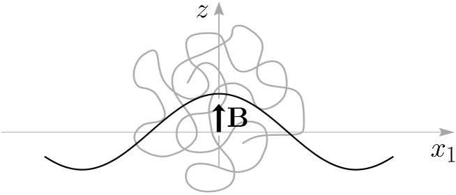
FIG. 3.: Sketch of the optimized translational shift B of the centre of mass of the chain for a sinusoidal surface profile.

Now the deflection factor can be approximated by

$$K[h(x)]=(1+|\nabla h(x)|^{2})^{1/2}\approx 1+{1\over 2}\int\limits_{0}^{\infty}\!{\text{d}}q\int\limits_{0}^{\infty}\!{\text{d}}q^{\prime}\,\tilde{h}(q)\,\tilde{h}(q^{\prime})\,qq^{\prime}\,\sin(qx)\,\sin(q^{\prime}x).$$ (33)

If additionally the part of the exponent in (24) and (25) which depends on $h(x)$ is expanded, we obtain in lowest order of $\tilde{h}(q)$

$$w_{1}^{\text{eff}} \approx w_{0}\,\left({G_{1}\over G_{3}}\right)^{3/2}\int\limits_{0}^{\infty}\!{\text{d}}q\int\limits_{0}^{\infty}\!{\text{d}}q^{\prime}\,\tilde{h}(q)\,\tilde{h}(q^{\prime})\,\exp\left\{-{G_{1}(q^{2}+{q^{\prime}}^{2})\over 2}\right\}\times$$ (35)

$$\qquad\times\,\left[q^{2}+{(q+q^{\prime})^{2}\over 2}\left(G_{3}qq^{\prime}\sinh(G_{1}qq^{\prime})-\cosh(G_{1}qq^{\prime})\right)\right]$$

$$w_{3}^{\text{eff}} \approx w_{0}\left\{1+{1\over 2G_{3}}\int\limits_{0}^{\infty}\!{\text{d}}q\int\limits_{0}^{\infty}\!{\text{d}}q^{\prime}\,\tilde{h}(q)\,\tilde{h}(q^{\prime})\,\exp\left\{-{G_{1}(q^{2}+{q^{\prime}}^{2})\over 2}\right\}\times\right.$$ (37)

$$\hskip 85.35826pt\times\,\Bigl{[}3+G_{3}qq^{\prime}\sinh(G_{1}qq^{\prime})-\cosh(G_{1}qq^{\prime})\Bigr{]}\Biggr{\}}$$

• A periodic surface geometry $\tilde{h}(q)=A_{h}\delta(q-f)$ leads to

  $$w_{1}^{\text{eff}} \approx w_{0}\,\left({G_{1}\over G_{3}}\right)^{3/2}{A_{h}^{2}f^{2}\over 2}\left\{G_{3}f^{2}\left(1-e^{-2G_{1}f^{2}}\right)-\left(1-e^{-G_{1}f^{2}}\right)^{2}\right\}$$ (38)

  $$w_{3}^{\text{eff}} \approx w_{0}\left\{1+{A_{h}^{2}f^{2}\over 4}\left(1-e^{-2G_{1}f^{2}}\right)-{3A_{h}^{2}\over 4G_{3}}\left(1-e^{-G_{1}f^{2}}\right)^{2}\right\}$$ (39)

  For a flat surface, the polymer extension $\bar{R}_{3}$ parallel to the mean surface normal (i.e. in $z$ direction) is identical to the size perpendicular to the surface. This is different for a rough surface profile, which now turns out to be important for the interpretation of (38) and (39). If for example $G_{3}$ is small compared with the squared wavelength $\lambda^{2}\simeq f^{2}$, then the polymer sticks to the surface, following the deflections. Therefore the result for $\bar{R}_{3}\simeq\sqrt{G_{3}}$ exceeds the polymer size perpendicular to the surface by the amount of the deflection, the effective interaction strength $w_{3}^{\text{eff}}$ accordingly is smaller than $w_{0}$. Adsorption enhancement therefore only can be obtained in the opposite case $\bar{R}_{3}\gg f^{-1}$, where the effective interaction strength parallel to the surface normal takes on its maximum value $w_{3\ \text{max}}^{\text{eff}}=w_{0}\{1+A_{h}^{2}f^{2}/4\}$.

  Here we have used $G_{1}\leq G_{3}$, which results from the fact that $w_{1}^{\text{eff}}$ always is small according to the condition $A_{h}f\ll 1$. As can be seen from (38), in the case $G_{3}\ll f^{-1}$ discussed above $w_{1}^{\text{eff}}$ is negative, so that the mean polymer extension in $x$ direction exceeds the size of a corresponding Gaussian chain, see (22).

• Similar to the case of a randomly distributed interaction strength, the amplitude in Fourier space $\tilde{w}^{\ast}(q)$ of a randomly distributed surface profile is identified with the square root of the spectral density $S(q)$. This means $\tilde{h}(q)=c^{-1}\,\Delta_{h}\,\exp\{-q^{2}\xi^{2}/2\}$ for a Gaussian distribution with mean $0$, variance $\Delta_{h}^{2}$ and correlation width $\xi$. In order to satisfy the requirement of weak disorder, we have to assume $\Delta_{h}^{2}\ll 1$ and $\xi\gg 0$. Then the result for the effective interaction strength in $z$ direction is

  $$w_{3}^{\text{eff}} = w_{0}\left\{1+\sqrt{{\pi\over 2}}{\Delta_{h}^{2}\over 4}\left[{G_{1}\over\xi^{3}}(2G_{1}+\xi^{2})^{-3/2}+{3\over G_{3}}\left((G_{1}+\xi^{2})^{-1}-{1\over\xi}(2G_{1}+\xi^{2})^{-1/2}\right)\right]\right\}.$$ (40)

  For a very large correlation width, which in the limit $\xi\to\infty$ corresponds to a flat surface, we again have the effect of a reduction of the effective interaction strength compared with the flat surface, $w_{3}^{\text{eff}}<w_{0}$. Therefore the result which is relevant for adsorption enhancement here is obtained in the case $\Delta_{h}\leq\xi^{2}\ll G_{3}\leq G_{1}$, where the effective interaction strength has its maximum value

  $$w_{3\ \text{max}}^{\text{eff}}\approx\ w_{0}\left\{1+{\textstyle c\,\Delta_{h}^{2}\over\textstyle\xi^{3}\sqrt{G_{1}}}\right\}.$$ (41)

  An analytic expression for $w_{1}^{\text{eff}}$ is not available, but the main features of the result can be estimated to strongly resemble those of $w_{1}^{\text{eff}}$ for a periodic surface profile discussed above.

IV Conclusions

The variational calculation presented here is valid for weak spatial disorder only (therefore it does not reproduce the scaling behavior for fractal surfaces). Nevertheless the mechanism of adsorption enhancement is well reproduced, we find agreement of the results in all special cases which were already investigated in the literature.

A special feature of the variational method employed here is the possibility of quantifying the localization transition, i.e., the transition from a slightly deformed Gaussian coil to a localized conformation, where the polymer size perpendicular to the surface no longer depends on the chain length. According to the result (21) the localization can be obtained by increase either of the effective interaction strength or of the chain length. This helps to compare the strength of adsorption enhancement for the two sorts of disorder considered here: as can be seen from the maximum values of (29) and (39) or from a comparison of (31) and (41), the localization transition is only slightly affected by a rough surface profile, whereas energetical heterogeneity can induce the transition even at vanishing mean interaction strength. Therefore we conclude that the disorder-induced enhancement of polymer adsorption is much more significant for a heterogeneous interaction strength than for spatial roughness.

Our findings concerning the localization behavior are affected qualitatively by the assumption of surface penetrability: for infinitely long chains at a flat and homogeneous impenetrable surface, the localization transition in contrast to (21) only occurs for some nonzero value of the attractive potential [1]. Nevertheless we expect our main statement on the significance of adsorption enhancement to hold also for impenetrable surfaces, since the comparison of transparent and opaque surfaces in simple soluble cases by Hone et al. [11] shows that they should not be affected differently by weak surface heterogeneities.

The polymer size parallel to the surface does not directly depend on the mean interaction strength, but only through the extension perpendicular to the surface. Thus, because it is less affected by heterogeneity, the former always exceeds the latter, except for one special case: for a flat, neutral surface with a periodic interaction strength, the polymer size parallel to the surface is smaller than perpendicular to it, if the period fits the polymer size such that it is concentrated to a maximum of $w(x)$ and even restricted by the neighboring repulsive regions.

V Acknowledgments

We would like to thank G. Heinrich for stimulating discussions. Financial support by the Deutsche Kautschuk Gesellschaft (DKG) is gratefully acknowledged.

REFERENCES

- [1] E. Eisenriegler, Polymers near surfaces, World Scientific, Singapur (1993)
- [2] G.J. Fleer et al., Polymers at interfaces, Chapman & Hall, London (1993)
- [3] G. Heinrich, T.A. Vilgis, Rubber Chem. Technol. 68 (1995), 26
- [4] T.A. Vilgis, G. Heinrich, Macromolecules 27 (1994), 7846
- [5] C.C. van der Linden, B. van Lent, F.A.M. Leermakers, G.J. Fleer, Macromolecules 27 (1994), 1915
- [6] D. Andelman, J.F. Joanny, J.Phys.II (France) 3 (1993), 121
- [7] A. Baumgärtner, M. Muthukumar, J. Chem. Phys. 94 (1991), 4062
- [8] M. Blunt, W. Barford, R. Ball, Macromolecules 22 (1989), 1458
- [9] R. Ball, M. Blunt, W. Barford, J. Phys. A: Math. Gen. 22 (1989), 2587
- [10] J.F. Douglas, Macromolecules 22 (1989), 3707
- [11] D. Hone, H. Ji, P.A. Pincus, Macromolecules 20 (1987), 2543
- [12] J.B. Donnet, R.C. Bansal, M.J. Wang (Eds.), Carbon black. Science and technology, Marcel Dekker, New York (1993)
- [13] B. Meissner, J. Appl. Polym. Sci. 50 (1993), 285
- [14] H.W. Diehl, A. Nüsser, Z. Phys. B 79 (1990), 69 & 79
- [15] T. Garel, H. Orland, Phys. Rev. B 55 (1997), 226
- [16] S.F. Edwards, M. Muthukumar, J. Chem. Phys. 89 (1988), 2435
- [17] S.F. Edwards, Y. Chen, J. Phys. A: Math. Gen. 21 (1988), 2963
- [18] M.E. Cates, R.C. Ball, J. Phys. France 49 (1988), 2009
- [19] P.G. de Gennes, Scaling concepts in polymer physics, Cornell University Press, Ithaca (1979)
- [20] J. Feder, Fractals, Plenum Press, New York (1988)
- [21] J. Klein, in Liquids at interfaces, Les Houches 1988 summer school XLVIII, J. Charvolin, J.F. Joanny, J.Zinn-Justin (Eds.), North Holland, Amsterdam, (1990)
- [22] A. Baumgärtner, M. Muthukumar, Adv. Chem. Phys. XCIV (1996), 625