Non-local effects in the fermion Dynamical mean field framework.
Application to the $2D$ Falicov-Kimball model.

Abstract

We propose a new, controlled approximation scheme that explicitly includes the effects of non-local correlations on the $D=\infty$ solution. In contrast to usual $D=\infty$, the selfenergy is selfconsistently coupled to two-particle correlation functions. The formalism is general, and is applied to the two-dimensional Falicov-Kimball model. Our approach possesses all the strengths of the large-$D$ solution, and allows one to undertake a systematic study of the effects of inclusion of ${\bf k}$-dependent effects on the $D=\infty$ picture. Results for the density of states $\rho(\omega)$, and the single particle spectral density for the $2D$ Falicov-Kimball model always yield positive definite $\rho(\omega)$, and the spectral function shows striking new features inaccessible in $D=\infty$. Our results are in good agreement with the exact results known on the $2D$ Falikov-Kimball model.

The effects of strong correlations on the properties of low-dimensional lattice fermion systems is still an open problem, inspite of many efforts spanning over thirty years. Recently, the development of a dynamical mean-field theory (DMFT), exact in $D=\infty$ has led to a major advancement in our understanding of the physics in the local limit[1, 2]. DMFT is a nonperturbative scheme. It has provided a detailed picture of the Mott transition in this limit, and has been fruitfully applied to a large class of models. Moreover, it has proved to be a rather good approximation to actual three-dimensional transition-metal and rare-earth compounds[2]. Inspite of its successes, DMFT has its shortcomings; the single particle selfenergy is ${\bf k}$-independent, and so is not coupled to ${\bf k}$-dependent collective excitations. This is clearly serious, e.g. near a magnetic phase transition where it cannot show any precursor effects. A consequence of the above is that the single particle spectral function cannot access such effects, and so the approach cannot be employed to describe e.g. angle-resolved photoemission experiments, or to study the changes in Fermi surface topologies driven by interactions in finite-$D$. The above makes it imperative to develop such controlled extensions of DMFT as are able to rectify its unphysical aspects, while preserving its strengths.

The DMFA maps the lattice system onto a selfconsistently embedded “impurity in a bath” problem that describes the effects of the coupling to other lattice sites. As in a Weiss mean field theory, a self consistency condition is obtained by requiring the averaged Green’s function of the bath $G_{0}$ to coincide with the local $G$ at this impurity site. DMFA becomes exact in $D=\infty$ because one can show that the spatial correlations fall off at least as $1/D^{|i-j|/2}$ with distance $|i-j|$ [4]. This “Weiss field” still has a nontrivial dynamics described by an effective local action $S_{DMF}$ obtained by integrating out all sites excluding the impurity site. Given $S_{DMF}$, one can compute the one particle Green’s function on this site, $G_{imp}(\omega)$, which is a functional of $G_{0}(\omega).$ The selfconsistency condition that links $G_{imp}$ back to $G_{0}$ is solved iteratively. The main drawback of this method is that $\Sigma$ is ${\bf k}$-independent.

In this letter, we present an extension of the DMFT that allows one to treat effects of non-local spatial correlations. To do so, we exploit the freedom involved in choosing the input bath propagator. We account for non-local correlations via the self consistent inclusion of two particle correlation function in the bath Green’s function (GF) $G_{0}(\omega)$. This is achieved by using the Spectral Density Approximation (SDA)[3]. Thus, our aim is to show that a proper combination of two methods –DMFT and SDA– is eminently suited to describe $1/D$ effects in lattice correlated fermionic systems. As far as application is concerned, we deal with the FKM as it was the first model to be solved exactly in $D=\infty$. Attempts at a $1/D$ expansion for the FKM have also been made. Finally, there exist some exact results on the $2D$ FKM which are of great help to evaluate the quality of our approximation, making it a first choice for testing methods in the context of extensions of the DMFT.

We now present this new method. We begin with the formalism for the generic Hubbard model at zero-temperature. We then go to the FK to solve the full set of selfconsistent equations. We will focus on half-filling, the extension away from $n=1$ is straightforward. The Hamiltonian is

$$H=-\sum_{<ij>,\sigma}t_{\sigma}(c_{i\sigma}^{{\dagger}}c_{j\sigma}+h.c)+U\sum_{i}n_{i\uparrow}n_{i\downarrow}-\mu\sum_{i\sigma}n_{i\sigma}$$

on a $D-$dimensional lattice. The Hubbard model is obtained when $t_{\uparrow}=t_{\downarrow}=t$, and the FKM is given by $t_{\uparrow}=t$ and $t_{\downarrow}=0$. In the case of half filling $\mu=U/2$ by particle-hole symmetry. These models have been extensively studied using the DMFT.

We get a bath propagator which includes $1/D$ effects using the SDA, first pioneered by Roth [3] to describe magnetism in narrow bands. Its basic idea is to compute exactly the first few moments of the spectral density to reconstruct the spectral function $A({\bf k},\omega)$. With H as above, it is easy to compute the first four moments. They are given by the expectation value of the following $n$-fold commutator

$$M_{{\bf k}\sigma}^{(n)}=<[...[[c^{\dagger}_{{\bf k},\sigma},H],H],...H]>$$ (1)

Using usual scaling arguments [4], one sees that the higher $n$, the higher will be the powers of $1/D$ involved in the $n$-th moment. In the case of a generic Hubbard model, it turns out that the $M_{{\bf k}\sigma}^{(3)}$ contains all the $o(1/D)$ contributions. It can be writen $M_{{\bf k}\sigma}^{(3)}=o(\frac{1}{D^{0}})+U^{2}n_{\downarrow}(1-n_{\downarrow})B_{{\bf k}\sigma}$ with

$$n_{\downarrow}(1- n_{\downarrow})B_{{\bf k}\sigma}=\frac{1}{N}\sum_{<ij>}\{t_{-\sigma}<c_{i-\sigma}^{{\dagger}}c_{j-\sigma}(1-2n_{i\sigma})>$$ (4)

$$-t_{\sigma}[<n_{i-\sigma}n_{j-\sigma}>-n_{-\sigma}^{2}-<c_{i\sigma}^{{\dagger}}c_{i-\sigma}^{{\dagger}}c_{j-\sigma}c_{j\sigma}>$$

$$-<c_{i\sigma}^{{\dagger}}c_{j-\sigma}^{{\dagger}}c_{j\sigma}c_{i-\sigma}>]e^{-i{\bf k}\cdot({\bf R_{i}}-{\bf R_{j}})}\}$$

The SDA then permits one to write an explicit closed form expression for $A_{\uparrow}({\bf k},\omega)=\delta[\omega-\epsilon_{\bf k}+\mu-\Sigma_{0,\uparrow}({\bf k},\omega)]$, where $\Sigma_{0,\uparrow}({\bf k},\omega)$ is given – for the generic Hubbard model – by

$$\Sigma_{0,\uparrow}({\bf k},\omega)=Un_{\downarrow}+U^{2}n_{\downarrow}(1-n_{\downarrow})[\omega+\mu-U(1-n_{\downarrow})-B_{{\bf k}\downarrow}]^{-1}$$

This is the self energy in the SDA. It is interesting to notice that all the order $1/D$ effects enter only through $B_{{\bf k}\sigma}$, whereby the self energy acquires a non-trivial ${\bf k}$-dependence. At this stage, this quantity is undetermined, and will have to be obtained self consistently. The SDA one particle Green’s function can then be computed as $G_{0\uparrow}({\bf k},\omega)=[\omega-\epsilon_{\bf k}-\Sigma_{0,\uparrow}({\bf k},\omega)]^{-1}$.

We now consider the FKM, ($t_{\downarrow}=0$). In this case, the model has a local $U(1)$ symmetry, $[n_{i\downarrow},H]=0$ $\forall i$. It thus follows from Elitzur’s theorem that only the second correlator in $B_{{\bf k}\sigma}$ is non zero. This leads to

$$n_{\downarrow}(1-n_{\downarrow})B_{{\bf k}\downarrow} =-\frac{t}{N}\sum_{<ij>}e^{-i{\bf k}\cdot({\bf R_{i}}-{\bf R_{j}})}[<n_{i\downarrow}n_{j\downarrow}>-n_{\downarrow}^{2}]$$ (6)

$$=-t\chi_{\downarrow}({\bf k})$$

where $\chi_{\downarrow}({\bf k})$ is the order $1/D$ static structure factor of the down spin electrons.

It is interesting to notice that the only order $1/D$ contribution to the single particle self energy is in fact $\chi_{\downarrow}({\bf q})$. The above equations are exact in the band as well as in the atomic limit, as can be easily checked. This has important consequences, for it points to a way for further improvement of the formalism. It allows one to formulate a DMFT for the local part, more or less along same lines as in $D=\infty$ [2]. However, in contrast to the regular DMFT where $\Sigma_{0\sigma}=0$, $G_{0}$ contains information about non-trivial ${\bf k}$-dependent features. Therefore, using this SDA $G_{0\sigma}$ as the input one particle bath Green’s function in a new DMFT scheme allows one to introduce in a simple way the non-local spatial fluctuations at order $1/D$ in the FKM.

We now come to the computation of the dynamical correlations. This results in a dynamically corrected self energy. To do this beyond the single-site level is a problem that has not been attempted, and here we use the standard DMFT as an approximation to the 2D case. In the case of the half filled FKM, the method drawn from the lines sketched above can be developed the following way.

As is known [6, 7], the equation-of-motion method (EOMM) gives the exact solution to the FKM in $D=\infty$. We will use the EOMM to get the full (local) impurity Green’s function which we denote by $G_{imp,\uparrow}(\omega)$.

The closed set of equations for the on-site Green’s function with a bath having $\Sigma_{0,\uparrow}({\bf k},\omega)$ as a selfenergy is given in ref. [7], replacing $\epsilon_{\bf k}$ by $\epsilon_{\bf k}+\Sigma_{0,\uparrow}({\bf k},\omega)$.

The local $G_{\uparrow}$ is computed to have the same form as that found in [2], and the local self-energy is computed from Dyson’s equation, $\Sigma_{imp,\uparrow}(\omega)=G_{0,imp,\uparrow}^{-1}(\omega)-G_{imp,\uparrow}^{-1}(\omega)$ where $G_{0,imp,\uparrow}(\omega)=[\omega+\mu-\Delta(\omega)]^{-1}$, with

$$\Delta(\omega)=\sum_{\bf k}\frac{t_{\bf k}^{2}}{\omega+\mu-\epsilon_{\bf k}-\Sigma_{0,\uparrow}({\bf k},\omega)}$$ (7)

One then gets

$$\Sigma_{imp,\uparrow}(\omega)=Un_{\downarrow}+\frac{U^{2}n_{\downarrow}(1-n_{\downarrow})}{\omega+\mu-U(1-n_{\downarrow})-\Delta(\omega)}.$$ (8)

This local dynamical self energy is used to correct the local part of the bath self energy, to introduce dynamical effects in the ${\bf k}$-dependent bath GF. This is done by

$$\Sigma_{\uparrow}({\bf k},\omega)=\Sigma_{imp,\uparrow}(\omega)+\Sigma_{0,\uparrow}({\bf k},\omega)-\sum_{\bf k}\Sigma_{0,\uparrow}({\bf k},\omega)$$ (9)

and provides us with a dynamically corrected non-local Green’s function $G_{\uparrow}({\bf k},\omega)=[\omega+\mu-\epsilon_{\bf k}-\Sigma_{\uparrow}({\bf k},\omega)]^{-1}$ which is exact in both the atomic and the band limits. The density of states is then obtained by taking the imaginary part of the ${\bf k}$-summed $G({\bf k},\omega)$.

To complete the procedure, one should selfconsistently compute the order $1/D$ correlator which enters the bath Green’s function as anounced earlier. In the case of the FKM, this means one has to compute the down spin static susceptibility. To begin with, we compute the vertex function exactly in $D=\infty$. The full $\chi_{\downarrow}({\bf q})$ is then obtained from the Bethe-Salpeter equation in the framework of the EOMM [6]. The result is $\chi_{\downarrow}({\bf q})=n_{\downarrow}(1-n_{\downarrow})/D({\bf q})$, where

$$D({\bf q})=1-\sum_{\nu}\frac{dn_{\downarrow}}{dG_{\nu}^{-1}}\left.\frac{\partial\Sigma_{\nu}}{\partial n_{\downarrow}}\right|_{G_{\nu}}\frac{G_{\nu}^{2}+\chi_{\uparrow}^{0}({\bf q})}{G_{\nu}^{2}[\chi^{0}_{\uparrow}({\bf q})\frac{d\Sigma_{\nu}}{dG_{\nu}}+1]}$$ (10)

and $\chi^{0}_{\uparrow}({\bf q})=(-1/N)\sum_{\bf k}G_{\uparrow}({\bf k}+{\bf q})G_{\uparrow}({\bf k})$, where the $\nu$-sum is on the Matsubara indices (we take the zero temperature limit). In the above, the vertex corrections in the equation for the charge susceptibility of the down-spins electrons are approximated by their $D=\infty$ values. To compute the vertex function exactly to order $1/D$ would be a formidable task, which has not been successfully attempted even for the electron gas.

FIG. 1.: (a) The selfconsistency loop in usual DMFT. (b) Our method: ${\bf k}$-dependent features are incorporated via an external input $\chi_{\downarrow}$ to the bath Green’s function $G_{0}$, which is computed self consistently as shown.

To sum up, the equations (6)-(10) above form a complete set of selfconsistent equations for the FKM. These include explicit $1/D$ effects through the ${\bf k}$-dependence of $\Sigma_{0,\uparrow}({\bf k},\omega)$. To solve these equations, we start with an arbitrary $\chi_{\downarrow}({\bf q})$ as an input in our initial $G_{0\uparrow}$. This is used to compute $\Sigma_{0,\uparrow}({\bf k},\omega)$, and the full $G_{imp,\uparrow}(\omega)$ from the large-$D$ solution along the lines of [7]. At this step, we have a DMF approximation to the FKM that is equivalent to a selfconsistent loop, with an external input quantity, the structure factor. The second step of our method is to compute $\chi_{\downarrow}({\bf q})$. For this purpose, we use the DMF approximation to the structure factor equation (10), plugging the obtained $G_{\uparrow}({\bf k},\omega)$ along with the full local vertex function in the Bethe-Salpeter equation to compute $\chi_{\downarrow}({\bf q})$. This is fed back into the equation for $\Sigma_{0,\uparrow}$ and the whole process is iterated to convergence. The difference between the regular self consistent DMFT and our method is illustrated in fig.1.

We implemented numerically this new method to study the Falicov-Kimball model on a $2D$ square lattice at $T=0$. The up spin electron dispersion relation is thus $\epsilon_{\bf k}=-2t(\cos{k_{x}}+\cos{k_{y}})$, and the corresponding density of states has a van Hove singularity at $\omega=0$. The ${\bf k}$ sums are performed on a $L\times L$ mesh, while the $\omega$-integrals are computed using standard integration procedures, using a small broadening $\eta$ to represent $\delta$ functions. Convergence is obtained when $\chi^{2}=\sum_{\omega}|G_{new}(\omega)-G_{old}(\omega)|^{2}<\varepsilon$ where $\varepsilon$ is a small threshold. At each step of the iterative process, a check on the accuracy of the computation is provided by the Luttinger sum-rule $\sum_{\bf k}\int_{-\infty}^{\mu}{\mbox{d}}\omega A_{\sigma}({\bf k},\omega)=n_{\sigma}$, which must be satisfied to high accuracy.

We now describe the results of our computation. Working with a lattice size $L=64$, and a threshold $\varepsilon=10^{-9}$, we observe a very fast convergence of the double selfconsistent procedure, that needs less than 10 steps to reach the convergence threshold for $G_{\uparrow}(\omega)$. The Luttinger sum rule is satisfied with an error of less than $10^{-3}$.

FIG. 2.: DOS for the $2D$ Falicov-Kimball model for several values of $U/t$ at half-filling, with our method. It is always positive definite. The inset shows the behavior of the $U/t=2$ gap at $\omega=0$ when changing the artificial broadening $\eta$ of the $\delta$ functions. $\eta/t=5.10^{-2}$ thick line, $\eta/t=5.10^{-3}$ thin line and $\eta/t=2.10^{-4}$ dashed line.

Fig.2 shows the density of states (DOS) $\rho(\omega)$ obtained by our method for several values of $U/t$. Firstly, notice that this function is always positive definite, in contrast to results of ref. [8]. This is a positive feature of the present method. We should stress that we are interested in the effect of coupling of self-energy to $1/D$ fluctuations, which, for the FKM, are completely static. The effect of the interaction is very clear. Starting from the $2D$ free fermions value at $U/t=0$, it opens a gap at $\omega=0$. The critical $(U/t)_{c}$ for opening up a gap is very small. As a matter of fact, working with a $L\times L$ lattice we cannot resolve energy details smaller than $2\pi v_{F}/L\simeq 0.2$ here. However, playing with the parameters of the problem, we see a real gap with $U/t$ as low as $0.1$. This result agrees with the exact result on the $2D$ FKM at weak coupling[11], where the gap and the related checkerboard order arises from the nested FS at $n=1$. The inset of fig.2 shows the behavior of the DOS at low frequency for $U/t=2$, obtained by changing the broadening of the delta functions to get a better precision. The features observed at higher frequencies are related to the unperturbed $2D$ band structure and are absent in infinite $D$.

The computed $\chi_{\downarrow}({\bf q})$, which contains information about long-range order (LRO), shows interesting behavior; along the zone-diagonal, at the point (${\bf k}=[\pi,\pi]$), it is a constant, scaling approximately with lattice size. This is the expected behavior in the broken-symmetry phase [12], and implies that the $n=1$ ground state is characterized by checkerboard LRO of the down-spin electrons [9]. In ref.[12], the behavior of $\chi_{\downarrow}({\bf q})$ can be studied only in $1D$, because of finite size restrictions. In contrast, our approach yields unambiguous conclusions in the thermodynamic limit in $2D$. Again, this is in clear agreement with the exact result[11].

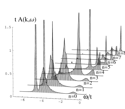
FIG. 3.: The spectral function $A_{\uparrow}({\bf k},\omega)$ for the $2D$ Falicov-Kimball model at half-filling, for $U/t=4$, and k along the zone diagonal, ${\bf k}=(n\pi/8,n\pi/8)$, $n$ going from 0 to 8.

The greatest advantage of our method, however, is that it allows a detailed study of ${\bf k}$-dependent (at the order of $1/D$) effects in the one particle spectral function $A({\bf k},\omega)=-{\rm Im}{G({\bf k},\omega)}/\pi$. In fig.3, we show $A({\bf k},\omega)$ for ${\bf k}$ along the zone-diagonal from ${\bf k}={\bf 0}$ to ${\bf k}=(\pi,\pi)$ for a representative value of $U=4t$. We notice that $A({\bf k},\omega)$ satisfies all the symmetry properties consistent with those expected from pure nearest neighbor hopping on bipartite lattices, and with particle-hole symmetry: $A({\bf k}_{0},\omega)=A({\bf k}_{0},-\omega)$ for ${\bf k}_{0}=[\pi/2,\pi/2]$, while along the zone diagonal $A({\bf k}_{0}+{\bf\delta},\omega)=A({\bf k}_{0}-{\bf\delta},-\omega)$, $\forall{\bf\delta}$ along the zone diagonal. We show only the $A({\bf k},\omega)$ for $\omega<0$; the $\omega>0$ part can be obtained from the symmetry property mentioned above. We have checked that our calculations are fully consistent with the above property. Moreover, we see that since ${\bf Q}=[\pi,\pi]$ is a nesting vector in $2D$, the above property of $A({\bf k},\omega)$ with ${\bf\delta}=[\pi/2,\pi/2]$ leads to a natural explanation of the “shadow-band” features observable in ARPES. It would be very interesting to see whether they survive away from $n=1$.

It is instructive to compare our results to those obtained by Velický et. al[10] in their pioneering paper on CPA. CPA is equivalent to the exact $D=\infty$ result for the FKM, and so a comparison with [10] allows us to study the effects of $1/D$ effects on $A({\bf k},\omega)$. A comparison of our data with results for identical parameters from [10] shows that the coupling to $1/D$ fluctuations induces new features in $A({\bf k},\omega)$ compared to those observed in DMFT. In $D=\infty$, $A({\bf k},\omega)$ has a two-peak structure with the dispersion controlled solely by the free bandstructure. In our approach, this is modified because of the extra ${\bf k}$-dependence coming through the $B_{{\bf k}\downarrow}$. This shows that a formalism capable of explicitly treating intersite correlations permits one to access ${\bf k}$-dependent features in $A({\bf k},\omega)$, so we suggest that this method can be fruitfully applied to compute ARPES lineshapes in correlated systems. A more detailed application to spectroscopy would require the use of the actual bandstructure DOS, and is left for future work.

In conclusion, we have developed a simple, physically appealing way to study the effects of non-local spatial fluctuations on the single particle spectral properties. We have applied the formalism to compute the single particle spectral function and the DOS for the $2D$ FKM and have obtained results in good accordance with what is known from the exact solution. Extensions of the work to look at the metallic phase in the FKM off $n=1$, as well as for the Hubbard model, are being studied and will be reported separately.

Mukul S.Laad wishes to thank the Alexander von Humboldt Stiftung for financial support during the time this project was started. We thank Prof. P.Fulde for advice and hospitality at the MPI, Dresden.

¹ e-mail: mukul@thp.uni-koeln.de

² e-mail: vdb@irsamc2.ups-tlse.fr

REFERENCES

- [1] J. Hubbard, Proc. Roy. Soc. (London) A281, 401 (1964).
- [2] A. Georges, G. Kotliar, W. Krauth and M. J. Rozenberg, Rev. Mod. Phys. 68, 13 (1996)
- [3] L. M. Roth, Phys. Rev. 184 , 461 (1969). For more recent work on SDA, see e.g. H. Beenen and D. M. Edwards, Phys. Rev. B52, 13636 (1995).
- [4] See D. Vollhardt, in Correlated electrons, edited by V. J. Emery, (World Scientific, Singapore, 1993)
- [5] S. Elitzur, Phys. Rev. D12 3978 (1975).
- [6] U. Brandt and C. Mielsch, Z. Phys B75 365 (1989)
- [7] M. Laad, Phys. Rev. B49 2327 (1994).
- [8] A. Schiller and K. Ingersent, Phys. Rev. Lett. 75 113 (1995).
- [9] See J. K. Freericks, Phys. Rev. B47, 9263 (1993), and ref. therein for numerical and analytical proofs of CDW order at half-filling.
- [10] B. Velický, S. Kirkpatrick and H. Ehrenreich, Phys. Rev. 175, 747 (1968).
- [11] A. Sütö, Ch. Gruber and P. Lemberger, J. Stat. Phys. 56 261 (1989), Ch. Gruber, J. Jedrzejewski, J. Iwanski and P. Lemberger Phys. rev. B41 2198 (1990).
- [12] P. Farkašovský, Z. Phys. B104 553 (1997)