Ordering of localized moments in Kondo lattice models

Abstract

We describe the transition from a ferromagnetic phase, to a disordered paramagnetic phase, which occurs in one-dimensional Kondo lattice models with partial conduction band filling. The transition is the quantum order-disorder transition of the transverse-field Ising chain, and reflects double-exchange ordered regions of localized spins being gradually destroyed as the coupling to the conduction electrons is reduced. For incommensurate conduction band filling, the low-energy properties of the localized spins near the transition are dominated by anomalous ordered (disordered) regions of localized spins which survive into the paramagnetic (ferromagnetic) phase. Many interesting properties follow, including a diverging susceptibility for a finite range of couplings into the paramagnetic phase. Our critical line equation, together with numerically determined transition points, are used to determine the effective range of the double-exchange interaction. Models considered are the spin 1/2 Kondo lattices with ferromagnetic and antiferromagnetic couplings, and the Kondo lattice with repulsive interactions between the conduction electrons.

]

I INTRODUCTION

The Kondo lattice model (KLM) describes the interaction between a conduction band and a lattice of localized spins. The hamiltonian for the KLM is

$$H=-t\sum_{<i,j>}\sum_{\sigma}c_{i\sigma}^{\dagger}c_{j\sigma}+J\sum_{j}{\bf S}_{cj}{\bf\cdot}{\bf S}_{j}\,,$$ (1)

where $t>0$ is the conduction electron (or simply electron) hopping, and $<i,j>$ denotes nearest neighbors. ${\bf S}_{j}$ are spin $1/2$ operators for the localized spins, and ${\bf S}_{cj}=\frac{1}{2}\sum_{\sigma,\sigma^{\prime}}c_{j\sigma}^{\dagger}{\mbox{\boldmath$\sigma$}}_{\sigma,\sigma^{\prime}}c_{j\sigma^{\prime}}$ are pseudospin operators for the conduction electrons. $\sigma$ are Pauli spin matrices, and $c_{j\sigma},c^{\dagger}_{j\sigma}$ the electron site operators. We choose units so that the hopping $t=1$, and measure the Kondo coupling $J$ in units of $t$. The KLM is an effective model for heavy-fermion systems when the coupling $J$ is small and positive [1], and models colossal magnetoresistance (CMR) materials when $J$ is large and negative [2].

In the following, we give a comprehensive description of the transition from a ferromagnetic (FM) ordering of the localized spins at stronger couplings, to a quantum disordered paramagnetic (PM) phase at weaker couplings. The transition has been identified in the one-dimensional (1D) KLM with partial conduction band filling both analytically [3], and in numerical simulations by a variety of methods [4, 5, 6, 7, 8]. We focus mainly on the $J>0$ 1D KLM relevant to heavy-fermion systems, in which the localized spins model $f$-electrons in lanthanide or actinide compounds. The bulk of the numerical simulations [4, 5, 6, 7] are devoted to this model. Partial conduction band filling $n=N_{c}/N<1$ is assumed throughout, where $N_{c}$ is the number of electrons, and $N$ the number of localized spins. Our approach generalizes to 1D KLMs with repulsive interactions between the electrons, and also to the KLM with a FM coupling $J<0$. These models are considered in Sec. IV.

A summary of our method is as follows: Abelian bosonization is used to describe the conduction band. Using a unitary transformation, the bosonized KLM is written in terms of a basis of states in which the localized spin and electron spin degrees of freedom are coupled. In the new basis, the competing interactions leading to the FM-PM transition are clearly exhibited. The competing effects are double-exchange FM ordering at stronger coupling, and spin-flip disorder processes at weaker coupling. Since the FM-PM transition is signalled by the ordering of the localized spins, we take expectation values for the electron Bose fields, and obtain an effective hamiltonian for the localized spins. The effective hamiltonian maps to a transverse-field Ising chain close to the FM-PM phase boundary, and we determine the critical line for the resulting quantum order-disorder transition, as well as many properties of the localized spins near criticality. At weak-coupling deep in the PM phase, the effective hamiltonian determines RKKY-like behavior, with dominant correlations in the localized spins at $2k_{F}$ of the conduction band.

The new element here is an emphasis on the double-exchange interaction, which tends to align the localized spins at stronger couplings. Double-exchange is often ignored in discussions of the $J>0$ KLM. Following its introduction 20 years ago by Doniach [9], the $J>0$ KLM has usually been discussed in terms of a competition between Kondo singlet formation, and the RKKY interaction. For the KLM with a half-filled conduction band $n=1$, this characterization appears sufficient. For the KLM with a partially-filled conduction band $n<1$, it has been realised that neither Kondo singlet formation, nor the RKKY interaction, are sufficient to describe rigorously established properties of the model [10]. A succession of analytic [11, 12, 3] and numerical [4, 5, 6, 7] results have established an extensive region of FM ordering at stronger coupling. This cannot be explained in terms of RKKY, which operates at weak-coupling, nor in terms of Kondo singlets, since they are non-magnetic. The missing element is double-exchange ordering due to an excess of localized spins over conduction electrons. Double-exchange requires only that $N>N_{c}$ (i.e. $n<1$), and that the conduction electron hopping $t\neq 0$. It operates in any dimension, for any sign of the coupling $J$, and for any magnitude $S_{j}^{2}$ of the localized spins [13]. The double-exchange interaction is specific to the Kondo lattice, and is absent in single- or dilute-impurity systems in which the situation is reversed, and the electrons greatly outnumber the localized spins.

Double-exchange is conceptually a very simple interaction: For $n<1$ each electron has on average more than one localized spin to screen, and consequently hops between several adjacent spins gaining screening energy at each site, together with a gain in kinetic energy. Since hopping is energetically most favorable for electrons which preserve their spin as they hop (called coherent hopping), this tends to align the underlying localized spins [13]. We show in Sec. II that coherent conduction electron hopping over a characteristic length $\alpha$ may be incorporated into a bosonization description which keeps the electrons finitely delocalized. At lengths beyond $\alpha$, the electrons are described by collective density fluctuations, as is usual in 1D Fermi systems. The electrons remain finitely delocalized over shorter lengths, and describe coherent hopping over several adjacent sites. This tends to align the underlying localized spins at stronger coupling. $\alpha$ measures the effective range of the double-exchange interaction, and is in principle a function of both filling $n$ and coupling $J$.

Our approach generates a ground-state phase diagram for the partially-filled 1D KLM in agreement with available exact and numerical results for the $J>0$ KLM [11, 12, 4, 5, 6, 7], for the $J>0$ KLM with repulsive interactions between the conduction electrons [14, 15], and for the KLM with a FM coupling $J<0$ [8]. Interesting new properties we determine include the following:
(i) For incommensurate conduction band filling, anomalous regions of double-exchange ordered localized spins survive close to the transition in the PM phase. Similarly, anomalous regions of disorder survive close to the transition in the FM phase. These regions exist due to the inability of the incommensurate conduction band to either totally order, or totally disorder the localized spins as the transition is crossed. Although the anomalous regions are very dilute, they dominate the low-energy properties of the localized spins. Many interesting results follow, including a diverging susceptibility in the PM phase for a finite range of couplings close to the transition.
(ii) The effective range of double-exchange ordering, measured by the length $\alpha$ for coherent electron hopping, is determined using our critical line equation together with numerically determined transition points. We find that $\alpha$ scales as $1/\sqrt{|J|}$ for any sign of the coupling $J$ on the transition line. For $J<0$, $\alpha\rightarrow 0$ as half-filling is approached; double-exchange is ineffective as $n\rightarrow 1$, and the transition line diverges. For $J>0$, $\alpha$ is reduced to less than a lattice spacing as $n\rightarrow 1$, but remains non-zero; the transition line remains finite close to half-filling for the $J>0$ KLM.

An outline of the paper is as follows: In Sec. II we derive the effective hamiltonian for the localized spins in the partially-filled $J>0$ 1D KLM, and provide a justification of results briefly reported elsewhere [3]. In Sec. III the effective hamiltonian is analyzed to determine the ground-state magnetic phase diagram, together with low-energy properties of the localized spins near the resulting FM-PM transition. Using our results, together with available numerical data, we determine the effective range of the double-exchange interaction on the transition line. Our method may be generalized to describe the FM-PM transition in other KLMs, and in Sec. IV we consider the 1D KLM with interactions between the electrons, and show that the FM-PM transition is pushed to lower values of $J$ for repulsive interactions. We consider also the KLM with a FM $J<0$ coupling, and follow a similar analysis to that for the $J>0$ case. The ground-state phase diagram is determined, together with the effective range of the double-exchange interaction on the resulting FM-PM transition line. The paper concludes in Sec. V with a summary of results, and a discussion of the general features of the FM-PM transition in partially-filled KLMs.

II EFFECTIVE HAMILTONIAN FOR THE LOCALIZED SPINS

A large class of 1D many-electron systems may be described using bosonization techniques [16]: The electron fields may be represented in terms of collective density operators which satisfy bosonic commutation relations. Bose representations provides a non-perturbative description which, in general, is far easier to manipulate than a formulation in terms of fermionic operators. In the 1D KLM, the conduction band may be bosonized, but not the localized spins. This is because the spins are strictly localized, and their Fermi velocity vanishes. Moreover, since there is no direct interaction between the localized spins in the KLM, it not possible to use bosonization via a direct Jordan-Wigner transformation. We therefore bosonize only the conduction band.

Bose representations are conveniently written in terms of Bose fields, defined as follows:

$$\phi_{\nu}(j) = -i\sum_{k\neq 0}\frac{\pi}{kL}[\nu_{+}(k)+\nu_{-}(k)]\Lambda_{\alpha}(k)e^{ikja},$$ (2)

$$\theta_{\nu}(j) = -i\sum_{k\neq 0}\frac{\pi}{kL}[\nu_{+}(k)-\nu_{-}(k)]\Lambda_{\alpha}(k)e^{ikja},$$ (3)

$$\Pi_{\nu}(j) = \frac{\pi}{L}\sum_{k\neq 0}[\nu_{+}(k)-\nu_{-}(k)]\Lambda_{\alpha}(k)e^{ikja}$$ (4)

$$= \partial_{x}\theta_{\nu}(j).$$ (5)

In Eqs. (5) $\nu=\rho,\sigma$ labels charge and spin, with charge and spin density operators

$$\rho_{r}(k)=\sum_{\sigma}\rho_{r\sigma}(k),\quad\,\,\sigma_{r}(k)=\sum_{\sigma}\sigma\rho_{r\sigma}(k).$$ (6)

$\sigma=\pm 1$ as the spin is up or down, respectively. The density operators $\rho_{r\sigma}(k)$ are the basic bosonic objects, and are defined by

$$\rho_{r\sigma}(k)=\sum_{0<rk^{\prime}<\pi/a}c^{\dagger}_{k^{\prime}-\frac{k}{2}\sigma}c_{k^{\prime}+\frac{k}{2}\sigma}\,.$$ (7)

The density operators describe collective coherent particle-hole excitations about the right ($r=+$) and left ($r=-$) Fermi points at $+k_{F}$ and $-k_{F}$, respectively. ($k_{F}=\pi n/2a$ with $a$ the lattice spacing. The system length is $L=Na$.) The density operators $\rho_{r\sigma}(k)$ are bosonic for wave vectors $|k|$ up to $\alpha^{-1}$. For these wave vectors we have [17]

$$[\rho_{r\sigma}(k),\rho_{r^{\prime}\sigma^{\prime}}(k^{\prime})]=\delta_{r,r^{\prime}}\,\delta_{k,-k^{\prime}}\,\delta_{\sigma,\sigma^{\prime}}\,\frac{rkL}{2\pi}\,.$$ (8)

In bosonization, $\alpha$ measures the minimum wavelength for the densities $\rho_{r\sigma}(k)$ which satisfy the bosonic commutation relations Eq. (8). Straightforward calculation, as in Ref. [17], shows that $\alpha$ must satisfy $\alpha\gtrsim{\cal O}(k_{F})^{-1}$. This is clear also on physical grounds; fermionic density operators are not collective, and hence cannot be bosonic, at wavelengths of the order of the average interparticle spacing. In the Bose fields of Eqs. (5), $\Lambda_{\alpha}(k)$ is a cut-off function on bosonic density operators. The cut-off function is an even function of $k$, and satisfies $\Lambda_{\alpha}(k)\approx 1$ when $|k|<\alpha^{-1}$, and $\Lambda_{\alpha}(k)\approx 0$ when $|k|>\alpha^{-1}$. $\Lambda_{\alpha}(k)$ ensures that only bosonic density operators enter the Bose fields. The commutation relations between the Bose fields are then c-numbers. The physical significance of the Bose fields is as potentials: $\partial_{x}\phi_{\nu}(j)$ is proportional to the $\nu$-density at site $j$, and $\partial_{x}\theta_{\nu}(j)=\Pi_{\nu}(j)$ is proportional to the average $\nu$-current at $j$. ($\partial_{x}\psi_{\nu}(j)$, $\psi=\phi,\theta$, is shorthand for $\partial_{x}\psi_{\nu}(x/a)$ evaluated at $x=ja$.)

Bose representations for Fermi operators are derived by requiring that they correctly reproduce the commutation relations of the Fermi operators with the density operators $\rho_{r\sigma}(k)$, and by requiring that they correctly reproduce the non-interacting ($J=0$) expectation values. Since the states generated by the density operators $\rho_{r\sigma}(k)$ span the 1D state space [18], this prescription ensures that the Bose representations will reproduce the same matrix elements as the original Fermi operators. In this way, the hopping term in Eq. (1) is given by

$$H_{0}=\frac{v_{F}a}{4\pi}\sum_{\nu,j}\left\{\Pi_{\nu}^{2}(j)+[\partial_{x}\phi_{\nu}(j)]^{2}\right\}\,,$$ (9)

with a linearized dispersion, and Fermi velocity $v_{F}=2a\sin(\pi n/2)$ in units of $t$. To bosonize the KLM, we also require representations for the on-site Fermi bilinears $c^{\dagger}_{j\sigma}c_{j\sigma^{\prime}}=\sum_{r,r^{\prime}}c^{\dagger}_{rj\sigma}c_{r^{\prime}j\sigma^{\prime}}$. The off-diagonal bilinears $c^{\dagger}_{rj\sigma}c_{r^{\prime}j\sigma^{\prime}}$, in which $r\neq r^{\prime}$ and/or $\sigma\neq\sigma^{\prime}$, may be constructed from the Bose representation for the single Fermi site operators

$$c_{rj\sigma} = \sqrt{Aa/2\alpha}\,\,\exp i[rk_{F}ja+\Psi_{r\sigma}(j)],$$ (10)

$$\Psi_{r\sigma}(j) = \{\theta_{\rho}(j)+r\phi_{\rho}(j)+\sigma[\theta_{\sigma}(j)+r\phi_{\sigma}(j)]\}/2,$$ (11)

where $A$ is a dimensionless constant depending on the cut-off function $\Lambda_{\alpha}(k)$. The representation Eq. (11) for $c_{rj\sigma}$ reproduces the correct commutation relations only with long-wavelength density operators $\rho_{r\sigma}(k)$. Thus the representation Eq. (11) may not correctly reproduce the short-range properties of the original conduction electron site operators $c_{j\sigma}$. The Bose representation for the diagonal on-site bilinears, i.e. the density operators in real space, may be obtained directly from their Fourier expansion:

$$\sum_{r}c^{\dagger}_{rj\sigma}c_{rj\sigma}=\frac{a}{2\pi}\partial_{x}[\phi_{\rho}(j)+\sigma\phi_{\sigma}(j)]$$ (12)

to an additive constant depending on $n$. As for $H_{0}$, and in constrast to $c_{rj\sigma}$, this representation is exact. Substituting these representations into Eq. (1) gives the bosonized KLM hamiltonian

$$H = \frac{v_{F}a}{4\pi}\sum_{j,\nu}\left\{\Pi_{\nu}^{2}(j)+[\partial_{x}\phi_{\nu}(j)]^{2}\right\}$$ (13)

$$+ \frac{Ja}{2\pi}\sum_{j}[\partial_{x}\phi_{\sigma}(j)]S_{j}^{z}$$ (14)

$$+ A\frac{Ja}{2\alpha}\sum_{j}\left\{\cos[\phi_{\sigma}(j)]+\cos[2k_{F}ja+\phi_{\rho}(j)]\right\}$$ (16)

$$\quad\quad\quad\quad\times\left(e^{-i\theta_{\sigma}(j)}S_{j}^{+}+{\rm h.c.}\right)$$

$$- A\frac{Ja}{\alpha}\sum_{j}\sin[\phi_{\sigma}(j)]\sin[2k_{F}ja+\phi_{\rho}(j)]S_{j}^{z}\,.$$ (17)

The bosonized hamiltonian generates the same behavior as the original hamiltonian provided that the conduction electrons are not strongly localized. In particular, the bosonized hamiltonian does not directly describe resonant on-site Kondo scattering: At strong-coupling the electrons localize, with each forming a Kondo singlet with the localized spin at the same site [19, 12]. The localized singlet formation is governed by the short-range properties of the spin-flip bilinears $c^{\dagger}_{j\sigma}c_{j-\sigma}$. However, the Bose representation for these terms, derived from Eq. (11), is reliable only at long-wavelengths. It describes the properties of a spin-flipped electron only at large distances from the scattering site. This provides a good description at weaker couplings, as usual in the bosonization of 1D Fermi systems, but may be insufficient when the coupling is strong enough that the electron becomes trapped on-site by the localized spin.

A second point to note about the bosonized hamiltonian concerns spin-rotation symmetry. $SU(2)$ symmetry is manifest in the original hamiltonian, Eq. (1), for both the electrons and the localized spins, but is obscured in the bosonized version. This is due to the use of abelian bosonization, which treats the electron spin $z$ direction on a special footing, and breaks the $SU(2)$ electron spin-rotation symmetry down to $U(1)$. To see the effect of this, note that the original hamiltonian preserves both the total spin $S_{\mbox{{tot}}}$ as well as its $z$ component $S^{z}_{\mbox{{tot}}}$, and at stronger couplings in the FM phase may be decoupled into subspaces with different values of $S^{z}_{\mbox{{tot}}}$. (See, for example, Ref. [12].) Abelian bosonization effectively singles out the subspace with maximal $S^{z}_{\mbox{{tot}}}$ in the FM phase (cf. Eq. (LABEL:tbklm) below), and may be physically motivated by crystal-field effects.

A Unitary transformation

A simple method for determining the ordering induced on the localized spins by the electrons is to choose a basis of states in which competing effects become more transparent. This is achieved by applying a unitary transformation which changes to a basis of states in which the conduction electron spin degrees of freedom are coupled directly to the localized spins. We choose the transformation

$$\exp({\rm S})\,,\quad{\rm S}=i\frac{Ja}{2\pi v_{F}}\sum_{j}\theta_{\sigma}(j)\,S_{j}^{z}\,.$$ (18)

A variant of this transformation was first used by Emery and Kivelson for the single-impurity Kondo problem [20], and was later generalized to the 1D KLM [21]. The usage here is different. Ref. [21] aimed to describe the conduction electrons, and the transformation was used to remove the spin current field $\theta_{\sigma}(j)$ from the hamiltonian. Here we aim to describe interactions between the localized spins, in which the electrons act as the mediators. The form of the transformation is then chosen so as to make explicit a FM ordering of the localized spins. This effect was entirely missed in the previous work [21]. The factor $Ja/2\pi v_{F}$ is chosen so that terms of the form $[\partial_{x}\phi_{\sigma}(j)]S_{j}^{z}$ exactly cancel in the transformed hamiltonian. This permits the ground-state $S_{j}^{z}$ configuration to be chosen independent of the on-site electron spin density in the transformed basis.

Transformed operators $\tilde{O}=e^{-{\rm S}}Oe^{{\rm S}}$ may be calculated using the standard commutator expansion

$$\tilde{O}=O+[O,{\rm S}]/1!+[[O,{\rm S}],{\rm S}]/2!+\cdots\;.$$ (19)

Using $[S_{j}^{x},S_{j^{\prime}}^{y}]=i\delta_{j,j^{\prime}}S_{j}^{z}$ etc., we get

$$\tilde{S}^{z}_{j} = S^{z}_{j}\,$$ (20)

$$\tilde{S}^{\pm}_{j} = S^{\pm}_{j}\exp\left\{\mp i\frac{Ja}{2\pi v_{F}}\theta_{\sigma}(j)\right\}$$ (21)

so that S rotates the localized spins in the $xy$-plane depending on the local electron spin current field. S does not alter the $S_{j}^{z}$ configuration. The only Bose field transformed under S is the electron spin density field, which takes a form that depends on the localized spin configuration all along the chain:

$$\tilde{\phi}_{\sigma}(j) = \phi_{\sigma}(j)+K(j)\,,$$ (22)

where $K(j)$ is a long-range object which essentially counts all the $S^{z}_{j^{\prime}}$ to the right of site $j$, and subtracts from that the $S^{z}_{j^{\prime}}$ to the left of $j$:

$$K(j) = i\frac{Ja}{2\pi v_{F}}\sum_{j^{\prime}}[\phi_{\sigma}(j),\theta_{\sigma}(j^{\prime})]S_{j^{\prime}}^{z}\,.$$ (23)

Here the Bose field commutator $[\phi_{\sigma}(j),\theta_{\sigma}(j^{\prime})]\rightarrow{\rm sign}(j-j^{\prime})\,i\pi$ for $(j-j^{\prime})a\gg\alpha$, and this provides the main contribution to $K(j)$. This term is discussed further in Sec. III. Related to the transformation of the spin density field is the transformation of the actual electron spin density at $j$. This depends on the local $S_{j^{\prime}}^{z}$ configuration. The transformed spin density $\widetilde{\partial_{x}\phi}_{\sigma}(j)$ is given by

$$\partial_{x}\phi_{\sigma}(j)-\frac{Ja}{\pi v_{F}}\sum_{j^{\prime}}\left\{\int_{0}^{\infty}dk\,\cos[k(j-j^{\prime})a]\Lambda_{\alpha}^{2}(k)\right\}S_{j^{\prime}}^{z},$$ (24)

The integral here is the Bose field commutator $i[\phi_{\sigma}(j),\Pi_{\sigma}(j^{\prime})]/2$, and is discussed further below.

After some manipulation, the above results give the transformed KLM hamiltonian

$$\tilde{H} = \frac{v_{F}a}{4\pi}\sum_{\nu,j}\left\{\Pi_{\nu}^{2}(j)[\partial_{x}\phi_{\nu}(j)]^{2}\right\}$$ (25)

$$- \frac{J^{2}a^{2}}{4\pi^{2}v_{F}}\sum_{j,j^{\prime}}\left\{\int_{0}^{\infty}dk\,\cos[k(j-j^{\prime})a]\Lambda_{\alpha}^{2}(k)\right\}S_{j}^{z}S_{j^{\prime}}^{z}$$ (26)

$$+ A\frac{Ja}{2\alpha}\sum_{j}\left\{\cos[K(j)+\phi_{\sigma}(j)]+\cos[2k_{F}ja+\phi_{\rho}(j)]\right\}$$ (28)

$$\quad\quad\quad\times\left(e^{-i(1+Ja/2\pi v_{F})\theta_{\sigma}(j)}S_{j}^{+}+{\rm{h.c.}}\right)$$

$$- A\frac{Ja}{\alpha}\sum_{j}\sin[K(j)+\phi_{\sigma}(j)]\sin[2k_{F}ja+\phi_{\rho}(j)]S_{j}^{z}$$ (29)

provided that the cut-off function is not too ‘soft’: $\Lambda_{\alpha}^{m}(k)\approx\Lambda_{\alpha}(k),m=2,3,4.$ (Discrepancies near $|k|\approx\alpha^{-1}$ introduce negligible corrections.) Note that the unitary transformation has been carried out exactly and not perturbatively, i.e. there has been no artificial truncation of the commutator series of Eq. (19). (The c-number Bose field commutators are essential for this.) It follows that the transformed hamiltonian of Eq. (LABEL:tbklm) is identical to the bosonized hamiltonian, and is an exact rewriting of Eq. (17) in terms of a new basis of states in which the conduction band and localized spins are interwoven.

B Double-exchange ordering

The important new term in the transformed hamiltonian Eq. (LABEL:tbklm) is the second:

$$-\frac{J^{2}a^{2}}{4\pi^{2}v_{F}}\sum_{j,j^{\prime}}\left\{\int_{0}^{\infty}dk\,\cos[k(j-j^{\prime})a]\Lambda_{\alpha}^{2}(k)\right\}S_{j}^{z}S_{j^{\prime}}^{z}\,.$$ (31)

It represents a non-perturbative effective interaction between the localized spins, and is the only one of this type to be derived for the KLM; other effective interactions, namely the RKKY interaction at weak-coupling, and the strong-coupling effective interaction of Sigrist et al. [12], are both perturbative. We consider FM in the KLM in some detail in this subsection. First we analyze the properties of the interaction described by Eq. (31), and describe how it arises from the bosonization of the conduction band. Second we present previously known properties of the double-exchange interaction. The interaction of Eq. (31) shares these properties, and we identify it as the double-exchange interaction in the KLM. Since double-exchange is usually not considered in discussions of the KLM with $J>0$, we conclude the subsection with a simple intuitive picture of double-exchange ordering in the KLM at low conduction band filling.

Eq. (31) possesses the following properties:
(i) the term originates, via bosonization and then the unitary transformation, from the terms $H_{0}$ and the forward scattering part of $(J/2)\sum_{j}(n_{j\uparrow}-n_{j\downarrow})S^{z}_{j}$ ($n_{j\sigma}=c^{\dagger}_{j\sigma}c_{j\sigma}$) in the KLM hamiltonian Eq. (1). (Note that the Bose representations for the electrons in these terms are exact.)
(ii) Eq. (31) is independent of the sign of $J$, and takes the same form for any magnitude $S_{j}^{2}$ of the localized spins.
(iii) Since Eq. (31) is of order $J^{2}$, whereas the remaining terms in the transformed hamiltonian Eq. (LABEL:tbklm) are of order $J$, the interaction Eq. (31) dominates the ordering of the localized spins as $J$ increases.
(iv) Eq. (31) is FM for all (differentiable) choices of the cut-off function $\Lambda_{\alpha}(k)$.
To give examples of the form of the FM interaction Eq. (31) in real space, consider Gaussian and exponential cut-off functions defined by $\Lambda_{\alpha}(k)=\exp(-\alpha^{2}k^{2}/2)$ for a Gaussian cut-off, and by $\Lambda_{\alpha}(k)=\exp(-\alpha|k|/2)$ for an exponential cut-off. For these cut-off functions, the integral in Eq. (31) reduces to

$$\int_{0}^{\infty}dk\,\cos(kja)\Lambda^{2}_{\alpha}(k)=(\sqrt{\pi}/2\alpha)\exp-(ja/2\alpha)^{2}$$ (32)

for the Gaussian, and

$$\int_{0}^{\infty}dk\,\cos(kja)\Lambda^{2}_{\alpha}(k)=\alpha/(\alpha^{2}+(ja)^{2})$$ (33)

for the exponential. The integrals are positive and non-negligible for $ja\lesssim\alpha$. The form of the FM interaction for Gaussian and exponential cut-off functions is shown in Fig. 1. It is clear that the length $\alpha$ characterizes the effective range of the FM interaction of Eq. (31).

FIG. 1.: The range in real space of the FM interaction Eq. (31) for exponential $\exp-(\alpha|k|/2)$ and Gaussian $\exp-(\alpha^{2}k^{2}/2)$ cut-off functions $\Lambda_{\alpha}(k)$. $J_{\mbox{{eff}}}$ is the interaction strength in units of $\alpha J^{2}a^{2}/4\pi^{2}v_{F}$.

The interaction Eq. (31) originates from the bosonization of the conduction band as follows: At wavelengths beyond $\alpha$, the electrons are involved in collective density fluctuations Eq. (7). These fluctuations involve large numbers of electrons, and satisfy bosonic commutation relations Eq. (8). This is the standard behavior of 1D many-electron systems for weak interactions. At wavelengths below $\alpha$, the density fluctuations are not collective, and do not satisfy bosonic commutation relations. Since bosonization describes fluctuations only over separations beyond $\alpha$, the bosonization description is equivalent to keeping the electrons finitely delocalized over $\alpha$, with the electrons preserving their spin over this range. Eq. (31) is the ordering consequently induced on the localized spins by the finitely delocalized electrons, and arises formally from the Bose field commutator $[\phi_{\sigma}(j),\Pi_{\sigma}(j^{\prime})]$. This commutator takes canonical $\delta$-function form in field theory [16], but is smeared over a range $\alpha\gtrsim{\cal O}(k_{F})^{-1}$ for the conduction band, which has a finite density $n$ of electrons. The smearing reflects the inability of the Bose fields to distinguish separations below $\alpha$.

We turn now to briefly summarize previously known properties of the double-exchange interaction. Double-exchange was first proposed many years ago by Zener [22] to explain FM ordering in mixed-valency manganites, and is of much current interest in relation to CMR materials [2]. The essential characteristic required for a system to exhibit double-exchange ordering is that the number of electrons be less than the number of localized spins. In this case, consider first infinitely strong coupling $J=\infty$. Each electron forms a perfectly localized on-site spin singlet (or triplet for $J<0$) with the localized spin at the same site. The remaining $N-N_{c}$ unpaired localized spins are free. When the conduction electron hopping is turned on, the electrons gain energy by hopping to unoccupied sites, since they gain energy both by screening the unpaired localized spin, together with a gain in kinetic energy. Since electrons tend to preserve their spin as they hop, called coherent hopping [2], this tends to align the underlying localized spins [13]. This is the double-exchange mechanism, and is generated by the conduction electron kinetic energy and the diagonal part of the on-site interaction between electrons and localized spins. Double-exchange is always FM, and dominates at stronger couplings [22]. It is the physical basis of the FM rigorously established in the 1D KLM by Sigrist et al. [11, 12]. (See also Ref. [10].) Since double-exchange ordering requires only $N>N_{c}$ and a non-vanishing hopping, its existence (as opposed to other properties such as its effective range) does not depend on the sign of $J$, nor on the magnitude of the localized spins. This is clear from the early analysis of Anderson and Hasegawa [13]; their result does not depend on the sign of $J$, except for some numerical prefactors, and is semiclassical with nearly trivial quantum modifications.

Properties (i)-(iv) above for the interaction of Eq. (31) are identical to those of a double-exchange interaction. This leads us to identify Eq. (31) as the double-exchange interaction in the partially-filled 1D KLM. Coherent conduction electron hopping, which generates double-exchange ordering, is described in the bosonization by electrons finitely delocalized over lengths $\alpha$, and $\alpha$ measures the effective range of the double-exchange interaction, as in Fig. 1. Note that $\alpha$ enters the bosonization description as an undetermined but finite length; from bosonization, we know only that $\alpha\gtrsim{\cal O}(k_{F})^{-1}$, and that in general $\alpha$ will be a function both of filling $n$ and coupling $J$ [17]. In Secs. III and IV (cf. Fig. 4), we determine $\alpha$ in a special case by using our results together with available numerical data.

Since many discussions of the $J>0$ KLM neglect the double-exchange interaction, it is useful to present the following simple characterization valid at low conduction band filling. Double-exchange may be described by the KLM hamiltonian Eq. (1) with spin-flip interactions ignored:

$$H_{\mbox{{de}}}=-t\sum_{j}\left(c^{\dagger}_{j\sigma}c_{j+1\sigma}+{\rm h.c.}\right)+J/2\sum_{j}(n_{j\uparrow}-n_{j\downarrow})S^{z}_{j}\,.$$ (34)

The occupation of a site by an electron with the same spin as the localized spin costs an energy $J/2$. We exclude these states as a first approximation valid at stronger couplings. At small filling, we consider a finitely delocalized electron of spin $\sigma$ spread over sites $j$ for which the localized spins $S^{z}_{j}$ have spin $-\sigma$ for $J>0$. From $H_{\mbox{{de}}}$, the wavefunction $\psi_{\sigma}(x)$ for the electron, in the continuum limit, satisfies the nonlinear Schrödinger equation

$$\partial^{2}_{x}\psi_{\sigma}(x)+(Jm/2)|\psi_{\sigma}(x)|^{2}\psi_{\sigma}(x)=2mE\psi_{\sigma}(x)$$ (35)

with $m$ the bare electron mass. The electron gains energy due to its occupation $|\psi_{\sigma}(x)|^{2}$ of a point with localized spin $S^{z}_{x}$ of spin $-\sigma$, and this generates the non-linearity. Finitely delocalized solutions of Eq. (35) are solitons with [23]

$$\psi_{\sigma}(x)=B\,e^{ix}\,{\rm sech}\left(B\sqrt{Jm/4}\,(x-x_{0})\right)\,.$$ (36)

B and $x_{0}$ are constants. Our simplified picture of the KLM at low conduction band filling is then of a gas of solitons. The solitons may be pictured as spin polarons [24, 11], and describe the dressing of each electron by a cloud of localized spins which align opposite to the conduction electron spin for $J>0$. The spatial extension of the polarization cloud characterizes the range of the indirect FM ordering induced on the localized spins by the electron, and is equivalent to the effective range $\alpha$ of the double-exchange interaction as described previously. From Eq. (36), the polarization cloud decays exponentially at large distances with a characteristic length scale proportional to $1/\sqrt{J}$. This gives a low density form $\alpha/a\propto 1/\sqrt{J}$. At vanishingly small fillings, we may use the exact solution of Sigrist et al. [11] for the KLM with one conduction electron. The polarization cloud decays exponentially for small $J$ in the FM phase, with a characteristic length $\alpha/a=\sqrt{2/J}$.

Since the interaction Eq. (31) is short-range for all finite $\alpha$ (correct for all finite $n$, cf. Fig. 4), we approximate it in the usual way by its nearest-neighbor form $-{\cal J}\sum_{j}S^{z}_{j}S^{z}_{j+1}$, where

$${\cal J}=\frac{J^{2}a^{2}}{2\pi^{2}v_{F}}\int_{0}^{\infty}dk\,\cos(ka)\Lambda^{2}_{\alpha}(k)\,.$$ (37)

We do not expect critical properties to be affected by this approximation.

C Effective hamiltonian

We aim to use the transformed hamiltonian Eq. (LABEL:tbklm) to determine the ground-state properties of the localized spins in the partially-filled 1D KLM. Our concentration on the localized spins is motivated by the results of numerical simulations on the KLM. Simulations on large chains have been carried out on the partially-filled 1D KLM using quantum Monte Carlo [4], and using the density-matrix renormalization-group (DMRG) [6, 7]. The results uniformly show that the correlations between the localized spins are much stronger than the correlations between the conduction electrons, and the FM-PM transition is signalled by the crossover from FM to incommensurate (generally $2k_{F}$) correlations in the structure factor of the localized spins. The corresponding electron correlations are observed to weakly track those of the localized spins, and the electron momentum distribution shows no dramatic change as the FM-PM transition line is crossed [6]. The freezing of the electron spin degrees of freedom occurs only at very strong coupling deep in the FM phase.

An effective hamiltonian for the localized spins is obtained from Eq. (LABEL:tbklm) by taking appropriately chosen expectation values for the conduction electron Bose fields. Since the Bose fields enter only in the weak-coupling terms of order $J$ in Eq. (LABEL:tbklm), we approximate the Bose fields by their non-interacting $J=0$ expectation values:

$$\langle\phi_{\nu}(j)\rangle_{0}=\langle\theta_{\sigma}(j)\rangle_{0}=0\,.$$ (38)

This holds for the charge density field $\phi_{\rho}(j)$, since at weak-coupling the charge structure factor is free electron-like [4]. For the spin fields, Eq. (38) follows from real-space renormalization-group studies [25], which show that the spin degrees of freedom of the 1D KLM flow to the non-interacting fixed point at weak-coupling. (This property is specific to the Kondo lattice [25]. For the single-impurity Kondo model at zero temperature, the spin coupling renormalizes to infinity for all $J\neq 0$.) Note that Eq. (38) is further supported by a study of the 1D KLM with $t$-$J$ interacting conduction electrons [15]. Using a combination of exact diagonalization and the DMRG, the same ordering was observed to be induced on the localized spins as in the pure KLM of Eq. (1), and confirms the insensitivity of the ordering to the details of the conduction electron behavior. The transformed hamiltonian Eq. (LABEL:tbklm) now reduces to an effective hamiltonian for the localized spins:

$$H_{\mbox{{eff}}} = -{\cal J}\sum_{j}S^{z}_{j}S^{z}_{j+1}$$ (39)

$$+ A\frac{Ja}{\alpha}\sum_{j}\{\cos[K(j)]+\cos[2k_{F}ja]\}S^{x}_{j}$$ (40)

$$- A\frac{Ja}{\alpha}\sum_{j}\sin[K(j)]\sin[2k_{F}ja]S^{z}_{j}\,.$$ (41)

III GROUND-STATE MAGNETIC PHASE DIAGRAM

In this section the effective hamiltonian $H_{\mbox{{eff}}}$ of Eq. (41) is analyzed to determine the ground-state properties of the localized spins as a function of conduction band filling $n$ and Kondo coupling strength $J>0$. Since the FM double-exchange coupling ${\cal J}$ is of order $J^{2}$ (cf. Eq. (37)), it is immediate from Eq. (41) that $H_{\mbox{{eff}}}$ determines a FM ordering for the localized spins at stronger couplings $J\gg 1$ for all fillings $n<1$. We find below that the FM ordering is gradually destroyed as the coupling $J$ is lowered. The destruction of the FM order is determined by the second term of Eq. (41); the effective hamiltonian takes the form of a transverse-field Ising chain in the phase transition region, and the KLM undergoes a quantum FM-PM transition at a filling dependent critical coupling $J_{c}$. The critical coupling is of order unity at most conduction band fillings. The determination of the FM-PM transition, and a disussion of the properties of the localized spins near the phase boundary, are contained in subsection IIIA. In subsection IIIB, we consider the weak-coupling regime $J\ll 1$. At weak coupling the double-exchange ordering is ineffective, and $H_{\mbox{{eff}}}$ reduces to a system of free localized spins in fields determined by conduction electron scattering (the last two terms of Eq. (41)). We find that $H_{\mbox{{eff}}}$ determines dominant $2k_{F}$ (RKKY-like) correlations in the localized spins at weak coupling. Finally, in subsection IIIC, we plot the ground-state phase diagram for the KLM as determined by the effective hamiltonian.

A The FM-PM phase transition

We begin our analysis of $H_{\mbox{{eff}}}$ by evaluating the long-range object $K(j)$ in the strong-coupling FM phase. $K(j)$, given by Eq. (23), originates with the unitary transformation S. It has some similarity to the disorder term in the Jordan-Wigner transformation, but instead of counting the $S^{z}_{j^{\prime}}$ only over sites to the left of $j$, it counts also the $S^{z}_{j^{\prime}}$ to the right. In the thermodynamic limit $N\rightarrow\infty$, and using the large $j-j^{\prime}$ form $[\phi_{\sigma}(j),\theta_{\sigma}(j^{\prime})]={\rm sign}(j-j^{\prime})\,i\pi$ for the Bose field commutator, we may rewrite Eq. (23) in the form

$$K(j)=\frac{Ja}{2v_{F}}\sum_{l=1}^{\infty}\epsilon_{j}(l)\,,$$ (42)

where $\epsilon_{j}(l)=S^{z}_{j+l}-S^{z}_{j-l}$. $\epsilon_{j}(l)$ has possible values $0,\pm 1$ for large $l$. For small $j-j^{\prime}$, the commutator $[\phi_{\sigma}(j),\theta_{\sigma}(j^{\prime})]$ grows smoothly from zero at $j=j^{\prime}$, to ${\rm sign}(j-j^{\prime})\,i\pi$ at $(j-j)={\cal O}(\alpha/a)$. The exact form of the commutator at short-range depends on the choice of cut-off function $\Lambda_{\alpha}(k)$, but all we require here is the general form: The effect of short-range corrections to the Bose field commutator is just to allow $\epsilon_{j}(l)$ to take values between $-1$ and $1$ for $l\lesssim\alpha/a$. $K(j)$ is then similarly smoothed, and takes values between integral multiples of $Ja/2v_{F}$.

By writing $K(j)$ in the form of Eq. (42), it is clear that $K(j)$ vanishes in the FM phase in a thermodynamically large system. Indeed $K(j)$ will not be appreciable until the system is strongly disordered. It follows that any transition out of the FM phase will be governed by the first two terms of the effective hamiltonian Eq. (41). For convenience we collect these terms in the hamiltonian $H_{\mbox{{crit}}}$ (with ‘crit’ for critical):

$$H_{\mbox{{crit}}}= - {\cal J}\sum_{j}S^{z}_{j}S^{z}_{j+1}$$ (43)

$$+ A\frac{Ja}{\alpha}\sum_{j}\{1+\cos(2k_{F}ja)\}S^{x}_{j}$$ (44)

$H_{\mbox{{crit}}}$ is a quantum transverse-field Ising chain, and a discussion of its properties occupies the remainder of this subsection. A great deal is already known about the transverse-field Ising chain, and the following discussion is essentially a summary of known results as they relate to the KLM. Of particular importance, it is known that $H_{\mbox{{crit}}}$ undergoes a quantum phase transition from a FM phase, to a disordered PM phase. We will outline how the transition is formally determined below, but before proceeding it is perhaps useful to consider the physics of the FM-PM transition in the KLM.

$H_{\mbox{{crit}}}$ describes the double-exchange FM ordering being gradually destroyed as the coupling $J$ is lowered. The first term of $H_{\mbox{{crit}}}$, which describes double-exchange, has been discussed extensively in subsection IIB above. The destruction of the double-exchange ordering may be understood physically as follows: As the coupling $J$ is decreased the conduction electrons become less strongly bound to the localized spins, and tend to extend over spatial ranges beyond the effective range $\alpha$ for double-exchange ordering. Double-exchange becomes less effective, and regions of ordered localized spins begin to interfere as the conduction electrons extend. The interference leads to spin-flip processes, and are embodied in $H_{\mbox{{crit}}}$ in the transverse-field (the second term of Eq. (44)). The transverse-field in $H_{\mbox{{crit}}}$ includes two low-energy spin-flip processes by which the conduction electrons disorder the localized spins. One spin-flip process is backscattering, and is accompanied by a momentum transfer of $2k_{F}$ from the conduction electrons to the localized spins. Since the chain of localized spins will tend to order so as to reflect this transfer, the transverse-field corresponding to backscattering spin-flips is sinusoidal with modulation $2k_{F}$. The other low-energy spin-flip process in $H_{\mbox{{crit}}}$ is forward scattering. This involves zero momentum transfer to the localized spins, and the corresponding transverse-field is a constant (i.e. has modulation zero).

It will become clear below that either forward or backscattering spin-flip processes separately are sufficient to destroy the FM order, and bring on a FM-PM phase transition in the KLM. However, for incommensurate conduction band filling, the backscattering spin-flip processes introduce a competing periodicity in the chain of localized spins. It turns out that this has non-trivial consequences for certain properties of the localized spins near the transition. In the following we first indicate how the FM-PM transition is determined for arbitrary transverse-fields. We then compare the properties of the localized spins which are disordered due to forward scattering (constant transverse-field), with the properties in which the spin disorder is due to backscattering (incommensurately modulated transverse-field). We point out that the special properties resulting from incommensurate backscattering are at least qualitatively reproduced by treating the full transverse-field in $H_{\mbox{{crit}}}$ as a random variable with the appropriate (displaced cosine) distribution. The subsection concludes with a summary of the properties of the random transverse-field Ising chain as they relate to the transition region in the KLM.

Determination of the phase transition

Using a Jordan-Wigner transformation to spinless fermions $a_{j},a^{\dagger}_{j}$, and in the thermodynamic limit, $H_{\mbox{{crit}}}$ may be written

$$H_{\mbox{{crit}}}=\sum_{j,l}\left\{a^{\dagger}_{j}A_{jl}a_{l}+\frac{1}{2}\left(a^{\dagger}_{j}B_{jl}a^{\dagger}_{l}+{\rm h.c.}\right)\right\}$$ (45)

to an additive constant, where $(A_{jl})$ and $(B_{jl})$ are real symmetric and antisymmetric matrices, respectively, with non-zero entries

$$A_{jj} = h_{j}\equiv A\frac{Ja}{\alpha}\{1+\cos(2k_{F}ja)\}$$ (46)

$$A_{jj+1} = A_{j+1j}=B_{jj+1}=-B_{j+1j}=-{\cal J}/4\,.$$ (47)

The quadratic form Eq. (45) may be diagonalized for any transverse-field $h_{j}$ by using the method of Lieb et al. [26]. This gives

$$H_{\mbox{{crit}}}=\sum_{k}\omega_{k}\eta^{\dagger}_{k}\eta_{k}$$ (48)

to an additive constant, where $\eta^{\dagger}_{k},\eta_{k}$ are creation and annihilation operators for free spinless fermions, and where the energies $\omega^{2}_{k}$ are eigenvalues of the symmetric matrix $(A+B)(A-B)$. As the coupling $J$ is decreased, $H_{\mbox{{crit}}}$ undergoes a quantum order-disorder transition from a FM phase, to a quantum disordered PM phase, signalled by the breakdown of long-range correlations between the localized spins, and a continuously vanishing spontaneous magnetization. The critical line for the transition is determined by the critical coupling $J_{c}$ which solves [27]

$${\cal J}^{N}-2^{N}\prod_{j=1}^{N}h_{j}=0$$ (49)

as $N\rightarrow\infty$. The free energy of the localized spins becomes non-analytic at points satisfying Eq. (49).

The FM-PM transition at the coupling $J_{c}$ is generic to transverse-field Ising chains, and does not assume a particular form for the transverse-field $h_{j}$ [27]. For example, if we consider only forward scattering spin-flip processes in the KLM, the transverse-field $h_{j}=AJa/\alpha$ is a constant. Solving Eq. (49) with $h_{j}=AJa/\alpha$ gives the quantum critical line for the FM-PM transition at

$$J_{c}=\frac{8\pi^{2}A\sin(\pi n/2)}{\alpha\int_{0}^{\infty}dk\,\cos(ka)\Lambda^{2}_{\alpha}(k)}\,.$$ (50)

A detailed discussion of the properties of the Ising chain with a constant transverse-field, which describes the FM-PM transition in the KLM with backscattering neglected, is given by Pfeuty [28]. As a second example, if we consider only backscattering spin-flip processes in the KLM, the transverse-field $h_{j}=AJa\cos(2k_{F}ja)/\alpha$ is sinusoidal. In real heavy-fermion materials, the number of available conduction electrons per localized spin will in general be irrational [29]. In this case the transverse-field due to backscattering has an incommensurate modulation $2k_{F}$ with respect to the underlying lattice of localized spins. Nonetheless a FM-PM transition still occurs. As shown in Ref. [30], the solution of Eq. (49) for incommensurately modulated transverse-fields yields a coupling $J_{c}$ as in Eq. (50) for the constant transverse-field. Thus the critical line for the FM-PM transition in the KLM with only backscattering spin-flip processes coincides with the critical line for the transition in the KLM with only forward scattering.

Effects of the form of the transverse-field

While the FM-PM transition itself is largely independent of the details of the transverse-field, there are significant differences in the properties of the localized spins on either side of the transition depending on the particular form of the transverse-field. The differences are most clearly apparent in the wavefunctions corresponding to the free fermions $\eta_{k}$ of the diagonalized hamiltonian Eq. (48). The wavefunctions are always extended, or Bloch-like, for a constant transverse-field [28]. For an incommensurately modulated transverse-field, the behavior of the wavefunctions is far more complex. The Ising chain with an incommensurate transverse-field has been studied extensively by Satija et al. [30, 31, 32]. The model is important as it has localized states in 1D, and thus provides a link to random systems [32]. Numerical studies [30] show that the wavefunctions corresponding to the free fermions $\eta_{k}$ are localized in the disordered PM phase, and undergo a spectral transition at the FM-PM phase boundary. In the FM phase, the wavefunctions are self-similar and the eigenvalue spectrum forms a Cantor set. Since the correlation functions for the localized spins are determined by the wavefunctions, the KLM with backscattering possesses far different properties to the KLM with only forward scattering spin-flip processes, even though both undergo a FM-PM transition. Differences in the eigenvalue spectrum $\omega_{k}$ of the diagonalized hamiltonian Eq. (48) lead to a similar conclusion regarding thermodynamic properties; since the KLM with incommensurate backscattering has a fractal eigenvalue spectrum, its thermodynamics are far different to the KLM with forward scattering, which has the more standard (cosine-type) eigenvalue spectrum [28].

The situation becomes yet more complex when we consider all possible low-energy spin-flip processes available to the conduction electrons. $H_{\mbox{{crit}}}$ includes forward scattering with zero momentum transfer, and is represented by a constant transverse-field. $H_{\mbox{{crit}}}$ also includes backscattering with an incommensurate momentum transfer $2k_{F}$, and is represented by a $2k_{F}$ sinusoidal transverse-field. $H_{\mbox{{crit}}}$ does not include spin-flip interactions with momentum transfers at higher harmonics of $2k_{F}$: at $4k_{F}$, $6k_{F}$, and so on. The higher harmonics will arise in a bosonization treatment which includes non-linear corrections to the conduction electron dispersion relation [16]. These corrections are very weak compared with the forward and backscattering spin-flip processes, and it is usual to neglect them. However, the addition of (even weak) higher harmonics in $2k_{F}$ to the transverse-field $h_{j}$ will greatly alter the solution of Eq. (49). Instead of one solution, there now occur an infinite number of solutions to Eq. (49), and these occupy a finite region of the parameter space [30]. The series of solutions is reflected in numerical studies on the Ising chain with a transverse-field containing more than one incommensurate harmonic [30, 31]. The region of spectral transitions becomes broadened, and the wavefunctions corresponding to the free fermions $\eta_{k}$ of Eq. (48) are observed to undergo a cascade of transitions between extended, critical, and localized behavior. The transitions in the wavefunctions occupy a finite region of the parameter space, and coincide with the solutions of Eq. (49) at which the free energy becomes non-analytic. While the region of spectral transitions becomes broadened, this is not the case for the magnetic transition. The FM-PM transition, signalled by the vanishing of longe-range correlations between the localized spins, is observed to remain sharp [31].

The behavior observed by Satija et al. in the numerical studies discussed above is qualitatively identical to the behavior of the Ising chain with a random transverse-field. (Properties of the random transverse-field Ising chain are disussed extensively by Fisher [33], and are summarized below.) To see this identification, note that the central feature of the random transverse-field Ising chain is that dilute regions of FM order may survive into the PM phase, and similarly that dilute regions of disorder may continue into the FM phase. This feature is at the heart of Fisher’s results [33], and is shared by $H_{\mbox{{crit}}}$ for incommensurate $k_{F}$: As discussed above, a broadened region of spectral transitions about the true FM-PM transition occurs in the KLM with incommensurate conduction band filling. Thus there are small regions in the PM phase in which the localized spins exhibit behavior normally associated with the FM phase, and vice versa. To further pursue the identification between a random transverse-field, and that present in $H_{\mbox{{crit}}}$ for the KLM, recall that the spectral transitions occur at points satisfying Eq. (49) at which the free energy becomes non-analytic. There is an immediate identification between these non-analytic points, and the Griffiths singularities [34] present in random models, in which thermodynamic quantities such as the magnetization become singular in a range of parameter space about the non-random transition. (See Ref. [33] for the Griffiths regions in the random transverse-field Ising chain.)

The behavior of $H_{\mbox{{crit}}}$ for incommensurate conduction band filling admits of a natural physical interpretation. The conduction band does not share the periodicity of the lattice of localized spins, and is unable to either totally order or totally disorder the lattice as the FM-PM transition is crossed. There remain dilute regions of double-exchange ordered localized spins into the PM phase as only a quasi-commensurate fraction of the conduction electrons become weakly-bound, and become free to scatter along the chain, at the FM-PM transition. The remaining ordered regions are dilute enough that no long range correlations remain, but their existence dominates the low-energy properties of the localized spins near the transition.

These considerations lead us to treat the transverse-field $h_{j}=AJa\{1+\cos(2k_{F}ja)\}/\alpha$ of $H_{\mbox{{crit}}}$ as a random variable, so that $h_{j}$ is chosen from the displaced cosine distribution $\rho(h)dh$ where

$$\rho(h)=\frac{\alpha}{\pi AJa}\frac{1}{\sqrt{1-(\alpha h/AJa-1)^{2}}}\,.$$ (51)

As discussed above, this treatment of $h_{j}$ does not alter the basic FM-PM transition described by $H_{\mbox{{crit}}}$, and thus is not needed in order to plot the phase diagrams of the KLM in Figs. 3 and 6 below. However, it does account for the properties of the localized spins near the FM-PM transition as observed by Satija et al. in their numerical simulations. We conclude by noting that at low conduction band filling the treatment of $h_{j}$ in Eq. (51) follows an analogous treatment in spin glass systems (cf. Ref. [3]).

Properties of the localized spins near criticality

Results on the random transverse-field Ising chain may be obtained from Fisher [33], who uses an approximate real-space renormalization-group (RG) analysis, which nonetheless yields asymptotically exact results at low-temperatures near criticality. Following Ref. [33], the critical coupling for the KLM is given by

$$J_{c}=\frac{4\pi^{2}A\sin(\pi n/2)}{\alpha\int_{0}^{\infty}dk\,\cos(ka)\Lambda^{2}_{\alpha}(k)}\,.$$ (52)

The critical line thus retains the form of Eq. (50) for forward or backscattering separately, but is down by a factor of 2 as both spin-flip disorder processes are included. It is convenient to measure deviations from criticality by [33]

$$\delta=\left[{\rm var}(\log h)\right]^{-1}\log\left\{\frac{4\pi^{2}A\sin(\pi n/2)}{J\alpha\int_{0}^{\infty}dk\,\cos(ka)\Lambda_{\alpha}^{2}(k)}\right\},$$ (53)

where the measure of randomness is

$${\rm var}(\log h)=\sum_{n=1}^{\infty}\left\{\frac{1}{n}\frac{1.3.\cdots.(2n-1)}{2.4.\cdots.(2n)}\sum_{m=1}^{2n-1}\frac{1}{m}\right\}-\log^{2}2\,.$$ (54)

$\delta=0$ on the critical line, is positive in the disordered PM phase, and negative in the FM phase.

The distinctive feature of Fisher’s RG analysis is that it focuses on anomalous clusters of double-exchange ordered localized spins which survive for small $\delta$ into the PM phase, and similarly, rare disordered regions close to criticality in the FM phase. These are due to the incommensurability of the conduction band filling with respect to the lattice of localized spins, and the consequent inability of the conduction band, as a single many-body entity, to either totally order or totally disorder the localized spins as the transition is crossed. It is the anomalous ordered (disordered) regions of localized spins in the PM (FM) phase which are responsible for the Griffiths singularities. Although these anomalous regions are very dilute, they dominate the low-energy properties of the spin chain. Thus, while typical correlations are much as in the constant transverse-field Ising chain, the measurable mean correlations are dominated by the anomalous regions, and consequently greatly alter the low-energy behavior.

An important prediction of our theory of the phase transition in the KLM is that the spontaneous magnetization grows continuously from criticality into the FM phase: For the random transverse-field [33]

$$M_{0}(\delta)\sim(-\delta)^{\beta}\,,\quad\quad\delta<0\,,$$ (55)

where $\beta=(3-\sqrt{5})/2\approx 0.38$ [35]. This disagrees with numerical diagonalization results on small systems [5], which see a discontinuous jump in $M_{0}$ at least at larger fillings, but note that regions of intermediate $M_{0}$ have been observed in related studies [15], and in small systems at lower fillings [5]. Indeed a discontinuous jump in $M_{0}$ immediately above the transition seems difficult to understand in a thermodynamically large system, given that the ordering is due to double-exchange, and that the electron spin degrees of freedom are not frozen until deep into the FM phase [6, 36].

Using Ref. [33], we summarize the properties of the 1D KLM which are relevant to the transition region of small $\delta$. The mean spin-spin correlation function is defined by

$${\overline{C}}(x)={\overline{\langle S^{z}_{j}S^{z}_{j+x}\rangle}}\,,$$ (56)

where the average is over $\rho(h)$, and where for convenience $x$ denotes a continuous and positive variable. ${\overline{C}}(x)$ is dominated by atypically large correlations and for small $|\delta|$ in the FM phase decays as

$${\overline{C}}(x)\sim M_{0}^{2}(\delta)+{\rm const.}|\delta|^{2\beta}(\xi/x)^{5/6}e^{-3(\pi x/\xi)^{1/3}}e^{-x/\xi}$$ (57)

for $x\gg\xi$. The correlation length $\xi\approx 1/\delta^{2}$. (For typical pairs of spins the correlation length $\xi\approx\delta^{-1}$; the exponent is the same as in the Ising chain with a constant transverse-field.) At criticality, $\delta=0$, the decay is power law: ${\overline{C}}(x)\sim x^{-\beta}$ as $x\rightarrow\infty$. For small $\delta$ in the PM phase,

$${\overline{C}}(x)\sim\delta^{2\beta}(\xi/x)^{5/6}e^{-(3/2)(2\pi^{2}x/\xi)^{1/3}}e^{-x/\xi}$$ (58)

where $x\gg\xi\approx 1/\delta^{2}$. Note that ${\overline{C}}(x)$ decays more rapidly to $M_{0}^{2}(\delta)$ in the FM phase, than it decays to zero in the PM phase.

At low temperatures $T$ close to the transition, ${\overline{C}}(x,T)$ decays exponentially at large distances with a correlation length $\xi_{T}$. In the FM phase, $\xi_{T}$ diverges as a continuously variable power law of $T$:

$$\xi_{T}\approx e^{2\Gamma_{T}|\delta|}/4\delta^{2}\quad\quad\Gamma_{T}|\delta|\rightarrow\infty$$ (59)

in the FM phase, where $\Gamma_{T}$ is a characteristic scale, given by $\Gamma_{T}=\log({\rm max}\{{\cal J},h_{j}\}/T)$ at fixed $J$ and $n$ close to the transition. At criticality the correlation length is $\xi_{T}\approx 4\Gamma^{2}_{T}/\pi^{2}$, while in the PM phase

$$\xi_{T}\approx(\delta^{2}+\pi/\Gamma_{T}^{2})^{-1}\quad\quad\Gamma_{T}\delta\gg 1\,.$$ (60)

The correlation lengths $\xi_{H}$ for the long-range exponential decay of the correlations ${\overline{C}}(x,H)$ in small applied fields $H$ along $z$ have identical functional forms to those of $\xi_{T}$ above. We note only that in the FM phase, $\xi_{H}\sim H^{-2|\delta|}$ as $H\rightarrow 0$. This reflects the development of long-range order, and shows a power law dependence on $H$. (See Fisher [33] for more details).

The magnetization in small positive applied fields $H$ along the $z$ direction is obtained [33] using an exact critical scaling function. Close to the critical line in the FM phase this gives

$$M(\delta,H)\sim M_{0}(\delta)[1+{\cal O}(\delta H^{2|\delta|}\log H)]$$ (61)

at zero temperature. At criticality, $M(\delta,H)\sim|\log H|^{-\beta}$, and in the PM phase

$$M(\delta,H)\sim\delta^{1+\beta}H^{2\delta}|\log H|\,.$$ (62)

Close to the transition in both phases the magnetization is highly singular. In the PM phase the magnetization has a power law singularity with a continuously variable exponent $2\delta$, and the linear susceptibility is infinite for a range of $\delta$ into the PM phase. The susceptibility remains infinite (with a continuously variable exponent) close to the transition into the FM phase. The low temperature linear susceptibility $\chi(T)$ takes the form

$$\chi(T)\sim T^{2\delta-1}(-\delta)^{-2(1-\beta)}$$ (63)

in the FM phase, and $T\chi(T)$ diverges as $T\rightarrow 0$. Note that the latter property was conjectured by Troyer and Würtz on the basis of their quantum Monte Carlo results [4]. At criticality, $\chi(T)\sim T^{-1}|\log T|^{2(1-\beta)}$, and close to the transition in the PM phase,

$$\chi(T)\sim\delta^{-4(1-\beta)}T^{2\delta-1}(\log T)^{2}.$$ (64)

$T\chi(T)$ vanishes as $T\rightarrow 0$ in the PM phase. The zero-field specific heat at low temperatures close to the transition is given by

$$C_{v}(T)\sim|\delta|^{3}T^{2|\delta|}[1+{\cal O}(T)^{2|\delta|}]$$ (65)

in either the FM or PM phases. At criticality, the specific heat $C_{v}(T)\sim|\log T|^{-3}$.

B Weak-coupling

Well below the transition, where $Ja/v_{F}$ is small and the FM interaction Eq. (31) is negligible, the ordering of the localized spins is governed by the last two terms of the effective hamiltonian Eq. (41). To determine the dominant correlations in this strongly disordered phase, it suffices to take eigenvalues for $\epsilon_{l}(j)$ in the long-range object $K(j)$ (cf. Eq. (42)). $K(j)$ then fluctuates about zero incoherently, depending on the global $S^{z}_{j}$ configuration. The effective hamiltonian corresponds to free localized spins in $x$ and $z$ fields determined by conduction electron scattering. The free localized spin problem is straightforwardly diagonalized by standard methods [37], and yields a ground-state $S^{z}_{j}$ configuration $|\psi_{0}\rangle$ given by

$$\exp\left\{i\sum_{j}\tan^{-1}\left(\frac{\cos[K(j)]+\cos(2k_{F}ja)}{\sin[K(j)]\sin(2k_{F}ja)}\right)S^{y}_{j}\right\}|\downarrow\rangle\,,$$ (66)

where $|\downarrow\rangle$ is the state with $S^{z}_{j}=-1/2$ for all $j$. The dominant $2k_{F}$ modulations in $|\psi_{0}\rangle$ are manifest, and are superimposed on an incoherent backgound:

$$\langle\psi_{0}|S^{z}_{j}S^{z}_{j+x}|\psi_{0}\rangle\approx\sin[2k_{F}ja]\sin[2k_{F}(ja+x)]$$ (67)

to an incoherent normalization. This is observed at weak-coupling in numerical simulations [4, 6, 7], and is called the RKKY regime. (Note, however, that the RKKY interaction strictly diverges in 1D, and there is no lower bound on the ground-state energy for the RKKY hamiltonian, even for arbitrarily small $J$ [12]. The divergence is typical of perturbation expansions in 1D, and does not occur in higher dimensions.)

C Phase diagram

The behavior identified in the previous subsections is in complete qualitative agreement with the results of numerical simulations on larger systems [4, 6, 7]. To establish quantitative agreement, i.e. to plot the critical line, we are presented with two obstacles. The critical line Eq. (52) with both forward and backscattering spin-flip interactions included may be written

$$J_{c}a=\frac{2\pi^{2}Av_{F}}{\alpha\int_{0}^{\infty}dk\,\cos(ka)\Lambda^{2}_{\alpha}(k)}\,.$$ (68)

The first obstacle in using Eq. (68) is somewhat trivial, and relates to the global scaling of the critical line: The number $A$ comes from the normalization of the Bose representations for spin-flip and backscattering electron interactions. It depends significantly on the cut-off function $\Lambda_{\alpha}(k)$, and moreover relates to the normalization of Bose representations only in the limit of long wavelengths (cf. Eq. (11)). The second obstacle is the dependence $\alpha=\alpha(n,J)$ which measures the effective range of the double-exchange interaction. This is a non-trivial quantity in a thermodynamically large system. In our previous work [3], we made the approximation of neglecting any functional dependence of $\alpha$ on $n$ and $J$, and determined $A$ by a fit to numerically determined points. The resulting phase diagram [3] correctly gives the general ground-state phase diagram of the KLM for $J>0$, and indicates schematically the regions where Griffiths singularities occur for incommensurate filling, together with the crossover to the strongly-disordered (RKKY-like) regime at weak-coupling. Here we provide a more detailed analysis, and use numerically determined phase transition points to determine the functional dependence of $\alpha$ on the critical line. Note that contrary to all previous results, the results of this subsection rely crucially on numerics.

We estimate first the constant $A$. From bosonization, we know that $\alpha\gtrsim{\cal O}(k_{F})^{-1}$, and so $\alpha$ will diverge as the filling $n\rightarrow 0$. From Eq. (68) it follows that

$$J_{c}\rightarrow 2\pi^{3}A\,n\,,\quad\,{\rm as}\,\,\,n\rightarrow 0\,.$$ (69)

Note the agreement with the exact solution of Sigrist et al. [11] for the KLM with one conduction electron; the system is FM for all finite $J$. Recall also that the exact solution gives $\alpha/a=\sqrt{2/J}$ for small $J$. It follows that $\alpha$ diverges at criticality in agreement with the result from bosonization as $n\rightarrow 0$. Using numerical results for $J_{c}$ at the smallest available filling ($J_{c}=0.455$ at $n=0.2$ from the infinite-size DMRG simulation of Caprara and Rosengren [7]), we conclude from Eq. (69) that $2\pi^{2}A\approx 0.7$.

FIG. 2.: Plot of the dimensionless parameter $Ja/v_{F}$, which characterizes double-exchange FM, against coupling $J>0$ for numerically determined FM-PM transition points $J_{c}$: the filled diamond is the quantum Monte Carlo result for systems up to 24 sites from Ref. [4]; open circles and squares are exact numerical diagonalization results for the 8 and 9 site chain, respectively, from Ref. [5]; the filled square is the DMRG result for systems up to 75 sites from Ref. [6]; the filled circles are infinite-size DMRG results from Ref. [7]. $J_{c}a/v_{F}\approx 0.7$ for vanishing $J$. The straight line of best fit is given, and shows good agreement with the spread of numerical results, together with the expected result as $J\rightarrow 0$.

We now account for the functional dependence of $\alpha$, and plot the critical line. $\alpha$ enters the critical line equation in the denominator of the right hand side of Eq. (68). This factor may be determined independently of a choice for the cut-off function $\Lambda_{\alpha}(k)$ by using numerically determined FM-PM transition points. In Fig. 2 we plot the dimensionless parameter $Ja/v_{F}$ against $J$ for available numerical data [4, 5, 6, 7]. $Ja/v_{F}$ characterizes double-exchange in our theory, and gives the denominator of Eq. (68) at criticality. The functional dependence is linear, and we give in Fig. 2 the straight line of best fit. This line gives $2\pi^{2}A=0.65$ as $n\rightarrow 0$, in agreement with the estimate $\approx 0.7$ from $n=0.2$ given in the previous paragraph. It is reasonable to conclude that the deviations in the numerically determined points for $Ja/v_{F}$ from the straight line are reflections of the different critical values determined in different simulations. The line of Fig. 2, together with Eq. (68), determines the critical line at

$$J_{c}=\frac{1.3\sin(\pi n/2)}{1-0.6\sin(\pi n/2)}\,,\quad\quad J>0\,.$$ (70)

The resulting phase diagram is given in Fig. 3.

FIG. 3.: Ground-state phase diagram of the 1D KLM with $J>0$. The critical line is from Eq. (70), and uses the line of Fig. 2. Numerically determined critical points are as in Fig. 2. At incommensurate fillings, there are Griffiths singularities in the free energy in a finite region of the parameter space about the critical line. At small $Ja/v_{F}$ in the paramagnetic phase, the system presents an RKKY-like behavior with dominant correlations in the localized spins at $2k_{F}$ of the conduction band.

The line of Fig. 2 determines the effective range $\alpha$ of the double-exchange interaction on the transition line. Choosing the exponential cut-off function $\Lambda_{\alpha}(k)=e^{-\alpha|k|/2}$ for simplicity, we have

$$\frac{1}{\alpha\int_{0}^{\infty}dk\,\cos(ka)\Lambda_{\alpha}^{2}(k)}=1+(a/\alpha)^{2}\,.$$ (71)

For this choice of cut-off function, the line of Fig. 2 gives $\alpha/a=\sqrt{2.1/J}$ at the transition. This compares with the result $\sqrt{2/J}$ obtained in the exact solution of the KLM with one conduction electron [11] just above the critical point at vanishing $J$. The filling dependence of $\alpha$ may be determined by using Eq. (70) to write $\alpha/a=\sqrt{2.1/J}$ in terms of $n$. The result is plotted in Fig. 4.

FIG. 4.: The effective range $\alpha$ of the double-exchange interaction in units of the lattice spacing against filling $n$ on the critical line. An exponential cut-off function $\Lambda_{\alpha}(k)=\exp-(\alpha|k|/2)$ has been chosen. The vanishing of the range at half-filling in the $J<0$ KLM leads to a divergence in the critical line as half filling is approached.

IV THE FM-PM TRANSITION IN RELATED MODELS

In this section we consider some variants of the 1D KLM of Eq. (1), and use our methods to describe the FM-PM transition at partial conduction band filling in these models. We consider firstly the effects of interactions between the electrons, and show that for repulsive interactions the phase boundary is always pushed to lower $J$ values, in agreement with available exact and numerical results [14, 15]. Second, we consider the KLM with a FM $J<0$ coupling. Our method extends to this model, and predicts the same class of phase transition as for $J>0$. Using available numerical results [8], we follow the analysis of Sec. III to determine the critical line and give the resulting phase diagram.

A Interacting conduction band

To determine the effects on the ordering of the localized spins due to interactions between the electrons, consider adding to the standard KLM hamiltonian of Eq. (1) the Hubbard interaction term

$$V=U\sum_{j}n_{j\uparrow}n_{j\downarrow}\,.$$ (72)

In terms of density operators, the interaction may be written

$$V = \frac{U}{4N}\sum_{k}[(\rho_{+}(k)+\rho_{-}(k))(\rho_{+}(-k)+\rho_{-}(-k))$$ (74)

$$\quad-(\sigma_{+}(k)+\sigma_{-}(k))(\sigma_{+}(-k)+\sigma_{-}(-k))],$$

where the charge and spin density operators are defined in Eq. (6). It will be sufficient for our purposes to consider only forward scattering contributions to $V$. (For weak repulsive interactions, $U$ small and positive, backscattering interactions renormalize to zero [38].) Within the Bose description, this is equivalent to attaching the weight $\Lambda_{\alpha}(k)$ to the density fluctuations in $V$. The interaction then reduces to standard Tomonaga-Luttinger–type, with forward scattering interactions described by bosonic density operators. The pure conduction band part $H_{0}+V$ of the interacting KLM may now be straightforwardly diagonalized via a Bogoliubov transformation $\exp({\rm S}_{B})$ where ${\rm S}_{B}=\sum_{\nu=\rho,\sigma}{\rm S}_{\nu}$ and

$${\rm S}_{\nu} = \frac{\pi}{2L}\log\left(\frac{v_{\nu}}{v_{F}}\right)$$ (75)

$$\times \sum_{k>0}\frac{1}{k}[\nu_{+}(k)\nu_{-}(-k)-\nu{-}(k)\nu_{+}(-k)]\Lambda_{\alpha}^{2}(k).$$ (76)

The charge and spin velocities are

$$v_{\rho} = v_{F}\sqrt{1+Ua/\pi v_{F}}\,\,,$$ (77)

$$v_{\sigma} = v_{F}\sqrt{1-Ua/\pi v_{F}}\,\,.$$ (78)

By comparison with the exact Bethe ansatz solution, these velocities are correct to leading order in $U$. Corrections to the velocities at stronger couplings are given by Schulz [39]. (Note that the spin velocity $v_{\sigma}$ does not go complex as $U$ increases, but smoothly goes to zero.) Under ${\rm S}_{B}$ the Bose fields transform as

$$\tilde{\phi}_{\nu}(j) = \sqrt{v_{F}/v_{\nu}}\,\phi_{\nu}(j),$$ (79)

$$\tilde{\theta}_{\nu}(j) = \sqrt{v_{\nu}/v_{F}}\,\theta_{\nu}(j),$$ (80)

while

$$\tilde{H}_{0} + \tilde{V}=\sum_{\nu=\rho,\sigma}H_{\nu},$$ (81)

$$H_{\nu} = \frac{v_{\nu}a}{4\pi}\sum_{j}\left\{\Pi_{\nu}^{2}(j)+[\partial_{x}\phi_{\nu}(j)]^{2}\right\}$$ (82)

to an additive constant. Under ${\rm S}_{B}$, the bosonized KLM with interactions between the electrons now takes the same basic form as the original bosonized hamiltonian of Eq. (17). The only differences are that the first term in Eq. (17) is replaced by $\sum_{\nu}H_{\nu}$, and that the Bose fields in the remaining terms are replaced by their scaled forms as in Eq. (80). Proceeding much as in the original $U=0$ problem, we choose the transformation $\exp({\rm S})$ where

$${\rm S}=i\frac{Ja}{2\pi}\sqrt{\frac{v_{F}}{v_{\sigma}^{3}}}\sum_{j}\theta_{\sigma}(j)\,S^{z}_{fj},$$ (83)

and obtain a transformed hamiltonian similar to Eq. (LABEL:tbklm). The important difference is that the prefactor of the double-exchange FM term of Eq. (31) is increased:

$$\frac{J^{2}a^{2}}{4\pi^{2}v_{F}}\rightarrow\frac{J^{2}a^{2}}{4\pi^{2}v_{F}}\,\frac{1}{1-Ua/\pi v_{F}}\,.$$ (84)

Following exactly the analysis of Sec. II, we obtain an effective hamiltonian for the localized spins. This determines a quantum order-disorder transition between FM and quantum disordered PM phases, with a critical coupling $J_{c}(U)$ which is down from the $U=0$ critical coupling by a factor $1-Ua/\pi v_{F}$. For stronger interactions between the conduction electrons, the spin velocity of Schulz [39] should be used in the transformation Eq. (83).

The effect of a repulsive Hubbard interaction between the electrons is then as follows. Double-exchange is characterized by the enhanced dimensionless constant $Ja\sqrt{v_{F}/v_{\sigma}^{3}}$. The FM phase becomes more robust, and the FM-PM phase boundary is pushed to lower values of $J$. We expect this on physical grounds: The repulsion between the electrons tends to keep the regions of double-exchange ordered localized spins from interfering. Spin-flip disorder processes are thereby reduced. Our result is consistent with the numerical work of Moukouri et al. [15] on the KLM with $t$-$J$ interacting electrons; reduced critical couplings $J_{c}\approx 0.8,1,1.2$ are determined for fillings $n=0.5,0.7,0.9$, respectively. Moreover, since $v_{\sigma}\rightarrow 0$ as $U\rightarrow\infty$ [39], so that $J_{c}\rightarrow 0$, our result coincides with the rigorous result of Yanagisawa and Harigaya [14] for infinite repulsive electron interactions.

B The KLM with a FM coupling

The KLM with a FM coupling $J<0$ is an effective model for CMR materials [2]. The localized spins in this model are three $t_{2g}$ Mn $d$-electrons, and have spin 3/2. The properties of the model of interest here are largely independent of the magnitude of the localized spins, and they may be approximated by spins 1/2 [2]. Noting that the double-exchange FM term Eq. (31) is insensitive to the sign of $J$, it may be readily verified that the derivation of the effective hamiltonian of Eq. (41) carries over to this case with minor modifications. This determines a quantum order-disorder transition from a FM to a disordered PM phase, with a critical line for $|J_{c}|$ given by Eq. (68).

To plot the critical line, we follow the analysis of Sec. III and use available numerically determined transition points for the $J<0$ KLM. Yunoki et al. [8] determine the FM-PM transition for classical spins via Monte Carlo, and for quantum spins 3/2 via the DMRG. The resulting transition lines, with coupling $J$ correspondingly scaled, are very close, and their points may be used within our spin 1/2 approximation. In Fig. 5 we plot the dimensionless parameter $Ja/v_{F}$ against $J$ for numerically determined points. The straight line of best fit gives very good agreement with the points, and as in Sec. III, determines the critical line

$$-J_{c}=\frac{0.7\sin(\pi n/2)}{1-\sin(\pi n/2)}\,.$$ (85)

The resulting phase diagram is given in Fig. 6. The critical line diverges close to half-filling, and differs from the $J>0$ KLM for which the line remains finite. We have not included the phase separated region identified by Yunoki et al. [8] in Fig. 6. Phase separation is observed in the classical spin simulation in the PM region from $J_{c}=4$. It is not observed in the quantum simulation until $J=6$, and then occurs away from the FM-PM transition closer to half filling. Any phase separation involves strongly localized electrons, and on-site localization is not described well by our bosonization of the conduction band (cf. Sec. II).

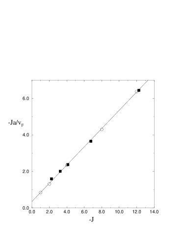
FIG. 5.: Plot of the dimensionless parameter $-Ja/v_{F}$, which characterizes double-exchange ordering in the $J<0$ KLM, against coupling $J$ for numerically determined FM-PM transition points: Open circles are results on classical localized spins using Monte Carlo on systems up to 40 sites from Ref. [8]; filled squares are DMRG results on a 16 site chain for quantum spins 3/2, and a correspondingly normalized coupling, from Ref. [8]. The straight line of best fit gives very good agreement with all points.

FIG. 6.: Phase diagram for the 1D KLM with a ferromagnetic coupling $J<0$. The critical line is from Eq. (85), and uses the line of Fig. 5. Numerically determined transition points are as in Fig. 5. Properties of the localized spins close to criticality and at weak-coupling are as for the $J>0$ KLM. The phase separated region identified in Ref. [8] for the classical spins from $J_{c}=4$ into the paramagnetic phase is not shown. Phase separation is observed in Ref. [8] in the quantum simulation only at stronger couplings, and away from the FM-PM transition closer to half filling.

The effective range $\alpha$ of the double-exchange interaction on the transition line may be determined as in Sec. III. For an exponential cut-off function, we find $\alpha/a=\sqrt{0.7/J}$. As a function of filling, this relation may be used together with the critical line Eq. (85) to plot $\alpha/a$ against $n$ as shown in Fig. 4. The vanishing of the effective range close to half filling is the reason the critical line diverges.

The different filling dependence of $\alpha$ for $J>0$ and $J<0$ is shown in Fig. 4. Different effective ranges $\alpha$ for the double-exchange interaction for different signs of the coupling is due to the different infinite $|J|$ symmetries of the sites containing localized conduction electrons. For a FM coupling, this is a triplet with energy $-|J|/4$, while for Kondo couplings $J>0$ the on-site symmetry is singlet with the lower energy $-3J/4$. The gain in energy for double-exchange per site and per conduction electron in either case is $-|J|/4$. For $J<0$, the system thus gains just as much energy from double-exchange as it does by forming localized triplets, and the triplets have minimal effect for a non-vanishing hopping. The effective range $\alpha$ vanishes smoothly as the number of excess localized spins declines: $\alpha\rightarrow 0$ as $n\rightarrow 1$. For $J>0$ the situation is far more complex. The on-site singlet energy is lower than the gain for double-exchange, and there is a complicated co-existence between the two effects. (This is why the exact solution for the KLM with one conduction electron is complex for $J>0$, whereas it is trivial for $J<0$ [11].) Fig. 4 indicates a saturation $\alpha\approx a$ as $n\rightarrow 1$ for $J>0$, in contrast to the $J<0$ behavior. We leave as an outstanding problem the reason for this: An accurate determination requires a detailed description of localized Kondo singlet formation on a par with the double-exchange ordering and weak-coupling spin-flip scattering which have been the focus here.

V DISCUSSION AND CONCLUSIONS

In this paper, we have described double-exchange FM ordering in the partially-filled 1D KLM, and the destuction of the FM phase by spin-flip disorder scattering. At weak-coupling deep in the disordered PM phase, the scattering determines RKKY-like correlations in the localized spins. Kondo singlet formation has been taken into account indirectly, via an effective range for the double-exchange interaction. The effective range was identified as follows: A length $\alpha\gtrsim{\cal O}(k_{F})^{-1}$ originates in bosonization as the minimum wavelength for density fluctuations which satisfy bosonic commutation relations. Bosonization describes fluctuations beyond $\alpha$, and keeps the conduction electrons finitely delocalized over lengths below $\alpha$. The electrons preserve their spin over this range. We showed in Sec. II that this finite delocalization may be identified with the length for coherent conduction electron hopping, and measures the effective range of the double-exchange FM ordering induced on the localized spins by the electrons (cf. Eq. (31) and Fig. 1). The reason this works is that double-exchange is conceptually a simple interaction. It reflects only the tendency for hopping electrons to preserve their spin, as they move to screen the more numerous localized spins. Double-exchange is characterized by the dimensionless factor $Ja/v_{F}$, with $v_{F}$ the conduction electron Fermi velocity and $a$ the lattice spacing.

We obtained a FM double-exchange interaction term Eq. (31) between the localized spins. The term was derived using a unitary transformation and is non-perturbative. This contrasts with other interactions derived for the localized spins in the KLM, such as the RKKY interaction, which are perturbative. The unitary transformation generates an effective hamiltonian Eq. (41) for the localized spins. The competing affects on the spin ordering are made manifest in the effective hamiltonian. The competing effects are double-exchange ordering at stronger coupling, and spin-flip disorder processes involving nearly free electrons at weak-coupling. The transition from a double-exchange ordered FM phase to a quantum disordered PM phase was then shown in Sec. III to be the quantum order-disorder transition of the transverse-field Ising chain (cf. Eq. (50)). This describes double-exchange ordered regions of localized spins being destroyed as the electrons become weakly-bound, and become free to move and scatter along the chain. As the coupling $J$ is lowered, the transition is signalled by a continuously vanishing spontaneous magnetization Eq. (55), and a breakdown in long-range correlations between the localized spins Eq. (58). The phase diagram is given in Fig. 3. Well below the critical line, no remnants of the ordering remain, and the effective hamiltonian describes dominant correlations in the localized spins at $2k_{F}$ of the conduction band.

Spin disorder occurs through forward and backscattering spin-flip processes between the electrons and the localized spins. We identified interesting properties resulting from an incommensurate modulation of the backscattering momentum transfer with respect to the underlying lattice of localized spins: For incommensurate fillings, the conduction band has a competing periodicity with respect to the spin chain, and the electrons are unable to totally order, or totally disorder the spin chain at criticality. This leaves anomalous regions of double-exchange ordered localized moments close to criticality in the PM phase, as only a quasi-commensurate fraction of the electrons become weakly-bound at the transition. Similarly, there remain anomalous disordered regions close to criticality in the FM phase. The anomalous regions are very dilute, but they dominate the low-energy behavior of the localized spins. The magnetization Eq. (62) is highly singular for a finite range of couplings about the critical line: The magnetization has a continuously variable power law exponent, and the susceptibility is infinite for a finite range of couplings even in the PM phase (cf. Eq. (64)).

We considered in Sec. IV the effect of conduction electron interactions on the FM-PM transition, and found that double-exchange is characterized by the dimensionless factor $Ja\sqrt{v_{F}/v_{\sigma}^{3}}$ for repulsive interactions, where $v_{\sigma}$ is the conduction electron spin velocity. This factor is enhanced (cf. Eq. (84)) over the factor $Ja/v_{F}$ characterizing double-exchange with no interaction between the conduction electrons. This pushes the critical line to lower values of the coupling $J$, and for infinitely strong repulsive interactions FM occupies the entire phase diagram for $J\neq 0$. The reason for this behavior is that for infinite repulsive interactions, the double-exchange ordered regions are prevented from interfering, and the spin-flip disorder processes are ineffective.

Since Kondo singlet formation is taken into account in our description only indirectly, our method extends also to the KLM with a FM $J<0$ coupling, and a FM-PM transition of the same class as $J>0$ was identified. The phase diagram for $J<0$ is given in Fig. 6. The difference between $J>0$ and $J<0$ is in the effective range $\alpha$ of the double-exchange interaction, and is due to the different energies for on-site triplets when $J<0$, to on-site Kondo singlets when $J>0$ (cf. Sec. IV). The effective range $\alpha$, which enters bosonization as a finite but unknown length, was determined at the FM-PM transition by using our critical line Eq. (68), together with numerically determined transition points [4, 5, 6, 7, 8]. We found that $\alpha/a\propto 1/\sqrt{|J|}$, in agreement with a simple characterization of double-exchange at small conduction band fillings (cf. Sec. II), and in agreement with an exact result [11] at vanishing filling. (Recall that the coupling $J$ is measured in units of hopping $t$). The proportionality constants are different for different signs of the coupling, and are fixed by a best fit to available numerically determined FM-PM transition points (Figs. 2 and 5). In Fig. 4 we plotted the corresponding filling dependence of $\alpha$ on the transition line: $\alpha\rightarrow 0$ as $n\rightarrow 1$ for $J<0$, but remains finite for $J>0$. This has a significant effect on the phase diagrams. For $J>0$ (Fig. 3) the critical line remains finite as $n\rightarrow 1$, while for $J<0$ (Fig. 6) the critical line diverges approaching half-filling. (Note that we do not consider the half-filled KLM. Indeed double-exchange FM is absent if the number of conduction electrons equals the number of localized spins.)

The transition we identified is generic to partially-filled spin 1/2 KLMs, at least in 1D. Our use of bosonization prevents us from anything more than speculation on the FM-PM transition in higher dimensional KLMs. We note only that (i) double-exchange is not restricted to 1D [22, 13], and should be considered in any discussion of partially-filled KLMs in higher dimensions. (ii) Numerical work [8] on the KLM with a FM coupling does present a FM-PM transition in higher dimensions, which is very similar to the transition in the 1D case.

We conclude with a simple physical picture, suggested to us by our results, which underlies the generic ground-state transition. At small fillings in the FM phase, spin 1/2 Kondo lattices form a gas of spin polarons, with each electron dressed by a cloud of ordered localized spins. The spatial extent of the polarization cloud is the effective range $\alpha$ for the double-exchange interaction. For $J>0$ the localized spins tend to align opposite to the spin of the conduction electron. For $J<0$ they tend to align parallel to the electron spin. As the coupling is lowered, the polarization clouds gradually extend and begin to interfere. The interference causes spin-flip disorder processes, which eventually destroy the FM order: The spin-flip processes free the electrons from their clouds of polarized localized spins, and this signals the onset of the FM-PM phase transition. At couplings just below the transition in the PM phase, the electrons are nearly free, and move through the system. They scatter from the localized spins as they move, and the spin chain is disordered. At weak-coupling, the localized spins retain dominant correlations at $2k_{F}$ of the conduction electrons, superimposed on an incoherent background. This reflects the momentum transferred from the conduction band to the spin chain in backscattering interactions, together with incoherent forward scattering.

REFERENCES

- [1] See, for example, P. A. Lee, T. M. Rice, J. W. Serene, L. J. Sham, and J. W. Wilkins, Comments Cond. Mat. Phys. 12, 99 (1986).
- [2] J. Zang, H. Röder, A. R. Bishop, and S. A. Trugman, J. Phys.: Condens. Matter 9, L157 (1997).
- [3] G. Honner and M. Gulácsi, Phys. Rev. Lett. 78, 2180, (1997).
- [4] M. Troyer and D. Würtz, Phys. Rev. B 47, 2886 (1993).
- [5] H. Tsunetsugu, M. Sigrist, and K. Ueda, Phys. Rev. B 47, 8345 (1993).
- [6] S. Moukouri and L. G. Caron, Phys. Rev. B 52, R15723 (1995).
- [7] S. Caprara and A. Rosengren, Europhys. Lett. 39, 55 (1997).
- [8] S. Yunoki, J. Hu, A. L. Malvezzi, A. Moreo, N. Furukawa, and E. Dagotto, cond-mat/9706014. See also E. Dagotto et al. cond-mat/9709029.
- [9] S. Doniach, Physica 91B, 231, (1977).
- [10] See, for example, T. Yanagisawa and M. Shimoi, Int. J. Mod. Phys. B 10, 3383 (1996).
- [11] M. Sigrist, H. Tsunetsugu, and K. Ueda, Phys. Rev. Lett. 67, 2211 (1991).
- [12] M. Sigrist, H. Tsunetsugu, K. Ueda, and T. M. Rice, Phys. Rev. B 46, 13838 (1992).
- [13] P. W. Anderson and H. Hasegawa, Phys. Rev. 100, 675 (1955).
- [14] T. Yanagisawa and K Harigaya, Phys. Rev. B 50, 9577 (1994).
- [15] S. Moukouri, L. Chen, and L. G. Caron, Phys. Rev. B 53, R488 (1996).
- [16] See, for example, J. Voit, Rep. Prog. Phys. 57, 977 (1994).
- [17] S. Tomonaga, Prog. Theor. Phys. 5, 544 (1950).
- [18] M. Schick, Phys. Rev. 166, 404 (1968).
- [19] J. E. Hirsch, Phys. Rev. B 30, 5383 (1984).
- [20] V. J. Emery and S. Kivelson, Phys. Rev. B 46, 10812 (1992).
- [21] O. Zachar, S. A. Kivelson, and V. J. Emery, Phys. Rev. Lett. 77, 1342 (1996).
- [22] C. Zener, Phys. Rev. 82, 403 (1951).
- [23] See, for example, V. G. Makhankov, Soliton Phenomenology, Mathematics and Its Applications (Soviet Series) Vol. 33 (Kluwer, Dordrecht, 1989).
- [24] T. Holstein, Ann. Phys. (N.Y) 16, 407 (1961).
- [25] R. Jullien, J. N. Fields, and S. Doniach, Phys. Rev. B 16, 4889 (1977).
- [26] E. Lieb, T. Schultz, and D. Mattis, Ann. Phys. (N.Y.) 16, 407 (1961).
- [27] P. Pfeuty, Phys. Lett 72A, 245 (1979).
- [28] P. Pfeuty, Ann. Phys. (N.Y.) 57, 79 (1970).
- [29] S. P. Strong and A. J. Millis, Phys. Rev. B 50, 9911 (1994).
- [30] I. I. Satija and M. M. Doria, Phys. Rev. B 39, 9757 (1989).
- [31] I. I. Satija, Phys. Rev. B 41, 7235 (1990).
- [32] I. I. Satija, Phys. Rev. B 49, 3391 (1994).
- [33] Daniel S. Fisher, Phys. Rev. Lett. 69, 534 (1992); Phys. Rev. B 51, 6411 (1995).
- [34] R. B. Griffiths, Phys. Rev. Lett. 23, 17 (1969).
- [35] For certain quasi-commensurate fillings, for example , the spontaneous magnetization still grows continuously, but the critical exponent may be reduced to its value 1/8 as in the constant transverse-field Ising chain. See Ref. [28].
- [36] Note that some features of the transition in the random transverse-field Ising chain are, however, loosely similar to those of first order transitions in random classical systems. See Ref. [33].
- [37] See, for example, M. Wagner, Unitary Transformations in Solid State Physics, Modern Problems in Condensed Matter Sciences Vol. 15 (Elsevier, Amsterdam, 1986).
- [38] See, for example, J. Sólyom, Adv. Phys. 28, 201 (1979), and references therein.
- [39] H. J. Schulz, Phys. Rev. Lett. 64, 2831 (1990); Int. J. Mod. Phys. B 5, 57 (1991).