Donnan equilibrium and the osmotic pressure of charged colloidal lattices

Abstract

We consider a system composed of a monodisperse charge-stabilized colloidal suspension in the presence of monovalent salt, separated from the pure electrolyte by a semipermeable membrane, which allows the crossing of solvent, counterions, and salt particles, but prevents the passage of polyions. The colloidal suspension, that is in a crystalline phase, is considered using a spherical Wigner-Seitz cell. After the Donnan equilibrium is achieved, there will be a difference in pressure between the two sides of the membrane. Using the functional density theory, we obtained the expression for the osmotic pressure as a function of the concentration of added salt, the colloidal volume fraction, and the size and charge of the colloidal particles. The results are compared with the experimental measurements for ordered polystyrene lattices of two different particle sizes over a range of ionic strengths and colloidal volume fractions.

PACS numbers: 82.70.Dd; 36.20.$-$r; 64.60.Cn

I Introduction

In recent years, colloidal particles have received an increased attention because they constitute an interesting system from practical, experimental, and theoretical point of view. Large molecules immersed in a solution are important in various systems, from biological to industrial. Due to the large size of the particles, a rich variety of experiments can be easily performed. Optical measurements show that some suspensions, such as the opals [1] and the viruses [2], form regular lattices that can, in principle, exhibit melting and structural phase transitions [3, 4]. The elastic rigidity of these ordered structures leads to unusual viscoelastic properties. The suspension responds to small-amplitude deformations as a linear viscoelastic solid, allowing for the propagation of the low-frequency shear waves [5, 6].

From the purely theoretical point of view, colloids are quite fascinating materials to study. Although thermodynamically identical to the usual atomic fluids and solids, colloids have an additional advantage in that the range of the interactions between the colloidal particles can be “manually” controlled by exploiting their interactions with a surrounding solvent, as well as by actually synthesizing particles which behave in a desired fashion. In general, the interactions between the colloids are dominated by a van der Waals force resulting from the quantum fluctuations of the electron charge density on the surface of a colloidal particle. This attractive interaction can lead to an aggregation of macromolecules and to their precipitation in a gravitational field. In many practical applications, such as design of water-soluble paints, it is essential to device a mechanism which would stabilize the colloidal suspension against precipitation. One such mechanism is to synthesize colloidal particles with some acidic groups on their surfaces, which will be ionized upon contact with water. The sufficiently strong electrostatic repulsion between the equally charged macromolecules will prevent the formation of clusters and stabilize the suspension against the precipitation. It is the aim of this paper to try and shed some light on the behavior of charge-stabilized colloids.

When the volume fraction is not too small, the charged polyions form an ordered structure (bcc or fcc) [7, 8, 9]. The description of the suspension in this case becomes significantly more simple than that of a disordered structure [10, 11, 12], since one can take advantage of the translational symmetry of the lattice. Thus each polyion, with its counterions, is inclosed in a Wigner-Seitz (WS) cell [7, 8, 9]. The thermodynamics of the system is then fully determined by the behavior inside one cell. In this paper we will present a simple theory to calculate the Donnan equilibrium properties of a charged colloidal lattice. The central problem will be to obtain the osmotic pressure of a colloidal crystal in equilibrium with a reservoir of salt. The experimental setup is described in Ref. [13]. It consists of an osmometer, which is made of two cells separated by a semipermeable membrane, which allows for the crossing of solvent, counterions, and the microions of salt, but prevents the passage of polyions. This, in turn, leads to an establishment of a membrane potential and an imbalance in the number of microions on the two sides of the membrane, resulting in an osmotic pressure measured by two capillaries attached to the chambers containing the colloidal suspension and the pure salt solution. This osmotic pressure, measured in mm of H₂O, will be compared to that found on the basis of our theoretical calculations.

II Osmotic pressure

Since the colloidal suspension is organized in a periodic structure, it is sufficient to consider just one isolated polyion in a salt solution inside an appropriate WS cell. To simplify the problem, a further approximation is to replace the polyhedral WS cell by a sphere of the same volume $V=\frac{\displaystyle 4\pi}{\displaystyle 3}R^{3}$, as represented in Fig. 1. Previous calculations, which compare explicitly results derived from the spherical-cell model with those that follow from a periodic system of cubic symmetry, show that this approximation provides a good description of the multibody system at low-volume fractions [7].

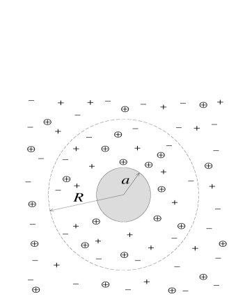
FIG. 1.: Geometry of the spherical Wigner-Seitz cell with radius $R$. The mesoscopic polyion (with total charge $-Ze$ distributed uniformly on its surface) is represented by the shaded sphere of radius $a$. The semipermeable membrane located at $|\mbox{\boldmath$r$}|=R$, represented by the dashed line, separates the polyelectrolyte from the pure solution of salt. The microscopic mobile ions — counterions $(\oplus)$, cations $(+)$ and anions $(-)$ — are free to move in the region $|\mbox{\boldmath$r$}|>a$, and can cross the semipermeable membrane.

Our theoretical picture, exploiting the underlying periodicity of the colloidal suspension [14], consists of a spherical polyion of radius $a$ with a uniform surface charge density,

$$q_{p}(\mbox{\boldmath$r$})=-\frac{\displaystyle Ze}{\displaystyle 4\pi a^{2}}\delta(|\mbox{\boldmath$r$}|-a)\>,\ \ \$$ (1)

residing at the center of a spherical WS cell, where $Z$ is the polyion valence, $e$ is the electronic charge and $\delta$ is the Dirac distribution. Note that we assume that the polyion is negatively charged. The boundary of the WS cell corresponds to the semipermeable membrane. The solvent, usually water, is modeled by a homogeneous continuum of a dielectric constant $\epsilon$. The mobile microions, modeled as point particles of charge $\pm e$, include the counterions and the ions derived from the dissociation of the monovalent salt, cations and anions. Inside the WS cell, these are free to move within the annulus $a<|\mbox{\boldmath$r$}|<R$. The distribution of microions is strongly determined by the electrostatic potential produced by the central polyion. In the region $|\mbox{\boldmath$r$}|>R$ the microions are assumed to be unaffected by the presence of the polyion at $|\mbox{\boldmath$r$}|=0$ and are uniformly distributed [15]. Within the functional density theory, the microions inside the WS cell are treated as an inhomogeneous fluid. At this level of approximation we shall not distinguish between the counterions and the cations of salt, so that the local density of positive particles is $\rho_{+}(\mbox{\boldmath$r$})$. The local density of co-ions (anions) is $\rho_{-}(\mbox{\boldmath$r$})$.

The effective Helmholtz free energy inside the WS cell, ${\cal F}^{\rm in}$, associated with the region of the colloidal suspension, is composed of:

(a) entropic ideal-gas contributions associated with the microion local densities $\rho_{\pm}(\mbox{\boldmath$r$})$,

$$\beta F^{\rm ideal}_{\pm}=\int d^{3}\mbox{\boldmath$r$}\,\rho_{\pm}(\mbox{\boldmath$r$})\left\{\ln\left[\rho_{\pm}(\mbox{\boldmath$r$})\Lambda^{3}\right]-1\right\}\>,\ \ \$$ (2)

where $\beta=(k_{B}T)^{-1}$ is the inverse temperature and $\Lambda=h/(2\pi mk_{B}T)^{1/2}$ is the thermal de Broglie wavelength;

(b) electrostatic energy terms due to the polyion-microions interactions,

$$F^{\rm el}_{p,\pm}=\pm e\int d^{3}\mbox{\boldmath$r$}\,d^{3}\mbox{\boldmath$r$}^{\prime}\,\frac{q_{p}(\mbox{\boldmath$r$})\rho_{\pm}(\mbox{\boldmath$r$}^{\prime})}{\epsilon|\mbox{\boldmath$r$}-\mbox{\boldmath$r$}^{\prime}|}\>;\ \ \$$ (3)

(c) electrostatic energy terms due to the microions-microions interactions,

$$F^{\rm el}_{ij}=e^{2}\int d^{3}\mbox{\boldmath$r$}\,d^{3}\mbox{\boldmath$r$}^{\prime}\,\frac{\rho_{i}(\mbox{\boldmath$r$})\rho_{j}(\mbox{\boldmath$r$}^{\prime})}{\epsilon|\mbox{\boldmath$r$}-\mbox{\boldmath$r$}^{\prime}|}\>,\qquad\mbox{ for }i,j=\pm\>;\ \ \$$ (4)

(d) and finally a (virtual) Lagrange-multiplier term,

$$F^{D}=\mu_{D}\int d^{3}\mbox{\boldmath$r$}\,\left[\rho_{+}(\mbox{\boldmath$r$})-\rho_{-}(\mbox{\boldmath$r$})\right]\>,\ \ \$$ (5)

which enforces the overall charge neutrality within the WS cell,

$$\int\limits_{a<|\mbox{\boldmath$r$}|<R}d^{3}\mbox{\boldmath$r$}\,\left[\rho_{+}(\mbox{\boldmath$r$})-\rho_{-}(\mbox{\boldmath$r$})\right]=Z\>.\ \ \$$ (6)

With the introduction of (5), we can treat the densities of microions, $\rho_{\pm}(\mbox{\boldmath$r$})$, as independent variables. The Lagrange multiplier $\mu_{D}$ is traditionally referred to as the Donnan potential. After the minimization procedure is complete, $\mu_{D}$ shall be eliminated using the charge-neutrality constraint (6). We have, then, the Helmholtz free energy inside the WS cell,

$${\cal F}^{\rm in} = F^{\rm ideal}_{+}+F^{\rm ideal}_{-}+F^{\rm el}_{p,+}+F^{\rm el}_{p,-}$$ (8)

$$+\frac{1}{2}F^{\rm el}_{++}+\frac{1}{2}F^{\rm el}_{--}-F^{\rm el}_{+-}+F^{D}\>.\ \ \$$

In the region outside the WS cell, the salt solution is, once again, charge neutral and the positive and negative ions are uniformly distributed. Due to this symmetry, the overall Coulombic contribution vanishes up to the correlation free energy, which we neglect within our treatment [15]. In the absence of an external field, the densities of positive and negative ions within the electrolyte chamber are uniform and given by

$$\rho_{+}(|\mbox{\boldmath$r$}|>R)=\rho_{-}(|\mbox{\boldmath$r$}|>R)=\rho_{S}\>,\ \ \$$ (9)

where $\rho_{S}$ is the (uniform) salt (cation/anion pairs) concentration of the pure electrolyte in the chamber after the equilibrium has been established. The Helmholtz free energy, $F^{\rm out}$, then reduces to that of an ideal gas,

$$\beta F^{\rm out}=V_{S}\,\rho_{+}\left[\ln\left(\rho_{+}\Lambda^{3}\right)-1\right]+V_{S}\,\rho_{-}\left[\ln\left(\rho_{-}\Lambda^{3}\right)-1\right]\,,\ \ \$$ (10)

where $V_{S}$ is the volume of the chamber containing pure electrolyte.

Assuming that the region outside the WS cell corresponds to the chamber containing the pure-electrolyte solution, the system will achieve the Donnan equilibrium when the electrochemical potentials inside,

$\!\rfloor$

$$\mu_{\pm}^{\rm in}(\mbox{\boldmath$r$})=\frac{\delta{\cal F}^{\rm in}}{\delta\rho_{\pm}(\mbox{\boldmath$r$})}=\frac{1}{\beta}\ln\left[\rho_{\pm}(\mbox{\boldmath$r$})\Lambda^{3}\right]\pm\mu_{D}\pm e\int d^{3}\mbox{\boldmath$r$}^{\prime}\,\frac{q_{p}(\mbox{\boldmath$r$}^{\prime})+e\rho_{+}(\mbox{\boldmath$r$}^{\prime})-e\rho_{-}(\mbox{\boldmath$r$}^{\prime})}{\epsilon|\mbox{\boldmath$r$}-\mbox{\boldmath$r$}^{\prime}|}=\frac{1}{\beta}\ln\left[\rho_{\pm}(\mbox{\boldmath$r$})\Lambda^{3}\right]\pm\mu_{D}\pm e\psi(\mbox{\boldmath$r$})\>,\ \ \$$ (11)

$\lceil\!$

and outside the WS cell,

$$\mu_{\pm}^{\rm out}=\frac{1}{V_{S}}\frac{\partial F^{\rm out}}{\partial\rho_{\pm}}=\frac{1}{\beta}\ln\left(\rho_{\pm}\Lambda^{3}\right)=\frac{1}{\beta}\ln\left(\rho_{S}\Lambda^{3}\right)\>,\ \ \$$ (12)

are equal,

$$\mu_{\pm}^{\rm in}(\mbox{\boldmath$r$})=\mu_{\pm}^{\rm out}\,.\ \ \$$ (13)

These conditions lead to the Boltzmann distribution of the microion densities,

$$\rho_{\pm}(\mbox{\boldmath$r$})=\rho_{S}\exp\left[\mp\beta\mu_{D}\mp e\beta\psi(\mbox{\boldmath$r$})\right]\>.\ \ \$$ (14)

On the other hand, the electrostatic potential $\psi(\mbox{\boldmath$r$})$ and the local charge densities obey the (exact) Poisson equation,

$$-\nabla^{2}\psi(\mbox{\boldmath$r$})=\nabla\cdot\mbox{\boldmath$E$}(\mbox{\boldmath$r$})=\frac{4\pi}{\epsilon}\left[q_{p}(\mbox{\boldmath$r$})+e\rho_{+}(\mbox{\boldmath$r$})-e\rho_{-}(\mbox{\boldmath$r$})\right]\>,\ \ \$$ (15)

where $\mbox{\boldmath$E$}(\mbox{\boldmath$r$})$ is the electric field at the point $r$, which is related to the electrostatic potential by $\mbox{\boldmath$E$}(\mbox{\boldmath$r$})=-\nabla\psi(\mbox{\boldmath$r$})$. Inserting expression (14) into Eq. (15) we find a Poisson-Boltzmann-like equation [16, 8, 7, 5, 17]. The effects of the correlations inside the ionic atmosphere can be included through the use of the local or the weighted-density contribution to the free-energy [7]. This will be a topic for the future.

We now take advantage of the spherical symmetry of the system to eliminate the angular dependence of the equations, that is, we replace $r$ by $r=|\mbox{\boldmath$r$}|$ in Eqs. (14) and (15). The electric field also has a spherical symmetry, so that $\mbox{\boldmath$E$}(\mbox{\boldmath$r$})=E(r)\frac{\displaystyle\mbox{\boldmath$r$}}{\displaystyle r}$. Integrating the Poisson equation (15) over a sphere of radius $r$ and using the divergence theorem, we obtain the equation for the electric field strength $E(r)$,

$$\int\limits_{|\mbox{\boldmath$r$}^{\prime}|<r}d^{3}\mbox{\boldmath$r$}^{\prime}\,\nabla\cdot\mbox{\boldmath$E$}(\mbox{\boldmath$r$}^{\prime}) = \int\limits_{|\mbox{\boldmath$r$}^{\prime}|=r}d\mbox{\boldmath$S$}^{\prime}\cdot\mbox{\boldmath$E$}(\mbox{\boldmath$r$}^{\prime})=4\pi r^{2}E(r)$$ (16)

$$= -\frac{4\pi Ze}{\epsilon}\left[1-\frac{1}{Z}\alpha(r)\right]\>,\ \ \$$ (17)

where

$$\alpha(r)=\int\limits_{|\mbox{\boldmath$r$}^{\prime}|<r}d^{3}\mbox{\boldmath$r$}^{\prime}\,\left[\rho_{+}(\mbox{\boldmath$r$}^{\prime})-\rho_{-}(\mbox{\boldmath$r$}^{\prime})\right]\>.\ \ \$$ (18)

Using the Boltzmann equations (14) for the densities of microions inside the WS cell, we can then write

$$\alpha(r)=4\pi\rho_{S}\left[\exp\left(-\beta\mu_{D}\right)\alpha_{+}(r)-\exp\left(\beta\mu_{D}\right)\alpha_{-}(r)\right]\>,\ \ \$$ (19)

where $\alpha_{\pm}(r)$ are the radial integrals associated with the electrostatic potential $\psi(r)$, that can be written in terms of the electric field strength $E(r)$,

$$\alpha_{\pm}(r) = \int_{a}^{r}dr^{\prime}\,r^{\prime 2}\,\exp\left[\mp e\beta\psi(r^{\prime})\right]$$ (20)

$$= \int_{a}^{r}dr^{\prime}\,r^{\prime 2}\,\exp\left[\pm e\beta\int_{a}^{r^{\prime}}dr^{\prime\prime}\,E(r^{\prime\prime})\right]\>,\ \ \$$ (21)

where we have chosen the gauge in which $\psi(r=a)=0$. The Lagrange multiplier $\mu_{D}$ can now be eliminated using the charge-neutrality constraint over the WS cell (6),

$\!\rfloor$

$$\alpha(R)=4\pi\rho_{S}\left[\exp\left(-\beta\mu_{D}\right)\alpha_{+}(R)-\exp\left(\beta\mu_{D}\right)\alpha_{-}(R)\right]=Z\>,\ \ \$$ (22)

which gives a quadratic equation for $\exp\left(-\beta\mu_{D}\right)$. Solving the associated equation and replacing in (19), we obtain

$$\alpha(r)=\frac{\sqrt{Z^{2}+(8\pi\rho_{S})^{2}\alpha_{+}(R)\alpha_{-}(R)}}{2}\left[\frac{\alpha_{+}(r)}{\alpha_{+}(R)}-\frac{\alpha_{-}(r)}{\alpha_{-}(R)}\right]+\frac{Z}{2}\left[\frac{\alpha_{+}(r)}{\alpha_{+}(R)}+\frac{\alpha_{-}(r)}{\alpha_{-}(R)}\right]\>.\ \ \$$ (23)

To perform the numerical calculations, it is convenient to write the equations in terms of dimensionless variables,

$$\hat{r}=\frac{r}{\lambda}\,,\qquad\hat{E}(\hat{r})=e\beta\lambda E(r)\,,\ \ \$$ (24)

$$\hat{\rho}_{\pm}(\hat{r})=4\pi\lambda^{3}\rho_{\pm}(r)\,,\qquad\hat{\rho}_{S}=4\pi\lambda^{3}\rho_{S}\,,$$ (25)

$$\hat{\alpha}_{\pm}(\hat{r}) = \frac{1}{\lambda^{3}}\alpha_{\pm}(r)=\int_{\hat{a}}^{\hat{r}}d\hat{r}^{\prime}\,\hat{r}^{\prime 2}\,\exp\left[\pm\int_{\hat{a}}^{\hat{r}^{\prime}}d\hat{r}^{\prime\prime}\,\hat{E}(\hat{r}^{\prime\prime})\right]\>,\ \ \$$ (26)

where we have introduced the Bjerrum length,

$$\lambda=\frac{\beta e^{2}}{\epsilon}\>,\ \ \$$ (27)

which measures the strength of the electrostatic interactions in the colloidal suspension.

The equation for the dimensionless electric field strength can be written as

$$\hat{E}(\hat{r})=-\frac{Z}{\hat{r}^{2}}\left[1-\frac{1}{Z}\hat{\alpha}(\hat{r})\right]\>,\ \ \$$ (28)

where $\hat{\alpha}(\hat{r})$ is given by Eq. (23), replacing $\alpha_{\pm}(r)$ by $\hat{\alpha}_{\pm}(\hat{r})$, and $8\pi\rho_{S}$ by $2\hat{\rho}_{S}$. Together with (23), this is an integral equation which determines the reduced electric field $\hat{E}(\hat{r})$. It is gauge invariant, since it does not depend on the choice for $\psi(r=a)$, and already contains the boundary conditions,

$$E(r=a)=-\frac{Ze}{\epsilon a^{2}}\>,\qquad\quad\mbox{and}\qquad\quad E(r=R)=0\>.\ \ \$$ (29)

This equation can be solved numerically by replacing the continuous interval $\hat{a}<\hat{r}<\hat{R}$ by a finite grid and iterating (28) until convergence is found. In the absence of added salt, $\hat{\rho}_{S}=0$, we regain the results of previous calculations [7, 8].

The dimensionless densities of microions inside the WS cell are given by

$$\hat{\rho}_{\pm}(\hat{r}) = \frac{\sqrt{Z^{2}+4\hat{\rho}_{S}^{2}\hat{\alpha}_{+}(\hat{R})\hat{\alpha}_{-}(\hat{R})}\pm Z}{2\hat{\alpha}_{\pm}(\hat{R})}\,\times$$ (31)

$$\times\,\exp\left[\pm\int_{\hat{a}}^{\hat{r}}d\hat{r}^{\prime}\,\hat{E}(\hat{r}^{\prime})\right]\>.\ \ \$$

The pressure inside the cell is $P^{\rm in}=-\frac{\displaystyle\partial\cal{F}^{\rm in}}{\displaystyle\partial V}=-\frac{\displaystyle 1}{\displaystyle 4\pi R^{2}}\frac{\displaystyle\partial\cal{F}^{\rm in}}{\displaystyle\partial R}$, which after some algebra reduces to [16]

$$\beta P^{\rm in}=\rho_{+}(R)+\rho_{-}(R)\>.\ \ \$$ (32)

The physical interpretation of (32) is that at the border of the WS cell the electrostatic forces on the mobile ions vanish, since $E(R)=0$, and the pressure is given by the ideal-gas law. On the other side of the membrane the charge is uniformly distributed and the pressure, up to the electrostatic correlations effects, is that of an ideal-gas,

$$\beta P^{\rm out}=-\beta\frac{\partial{F}^{\rm out}}{\partial V_{S}}=2\rho_{S}\>.\ \ \$$ (33)

Therefore, the osmotic pressure, defined as the difference between the pressures inside and outside the WS cell, is

$$\beta\Delta P = \beta P^{\rm in}-\beta P^{\rm out}=\rho_{+}(R)+\rho_{-}(R)-2\rho_{S}$$ (34)

$$= \frac{1}{4\pi\lambda^{3}}\left[\hat{\rho}_{+}(\hat{R})+\hat{\rho}_{-}(\hat{R})-2\hat{\rho}_{S}\right]\>.\ \ \$$ (35)

III Comparison with experimental results

The derivation in the previous section requires us to know the concentration of salt $\rho_{S}$ once equilibrium across the membrane has been established. Although, in principle, this is possible to measure, it is much simpler, from the point of view of experiment, if the osmotic pressure was calculated as a function of the concentrations of salt present in the two chambers, $n^{0}$ and $\rho_{S}^{0}$, before the ion transport is allowed to take place. Evidently it is these values that are directly controlled by the experimentalist. In this section we will present the results for the osmotic pressure as a function of the original concentration of salt added to the polyelectrolyte in the first chamber, $n^{0}$, and of the initial pure-electrolyte concentration in the second chamber, $\rho_{S}^{0}$, before the ion transport is allowed to take place. In this way our results can be directly compared with the measurements of Benzing and Russel [6].

The initial concentration of salt in the pure-electrolyte chamber, $\rho_{S}^{0}$, will not coincide with the same quantity $\rho_{S}$ measured after the Donnan equilibrium is achieved. A relation between these two concentrations can, however, be determined through a mass-conservation condition as follows. If $n^{0}$ and $n$ are the (macroscopic) average salt concentrations in the colloidal-suspension chamber before and after the Donnan equilibrium is achieved, and $V_{C}$ and $V_{S}$ are the volumes of the colloidal-suspension and the pure-electrolyte chambers, then the mass-conservation condition,

$$n^{0}V_{C}+\rho_{S}^{0}V_{S}=nV_{C}+\rho_{S}V_{S}\>,\ \ \$$ (36)

or

$$n=n^{0}(1+\gamma_{1}\gamma_{2})-\gamma_{1}\rho_{S}\>,\ \ \$$ (37)

gives a relation between the average concentrations of salt in the suspension after and before the equilibrium in terms of the ratios

$$\gamma_{1}=\frac{V_{S}}{V_{C}}\qquad\quad\mbox{ and }\qquad\quad\gamma_{2}=\frac{\rho_{S}^{0}}{n^{0}}\>.\ \ \$$ (38)

Since the microions are just allowed to occupy an effective volume of the WS cell,

$$V_{\rm eff}=\frac{4\pi}{3}(R^{3}-a^{3})=\frac{4\pi\lambda^{3}}{3}\hat{R}^{3}(1-\phi)\>,\ \ \$$ (39)

where $\phi$ is the volume fraction occupied by the polyion,

$$\phi=\left(\frac{a}{R}\right)^{3}\>,\ \ \$$ (40)

it is useful to define an effective salt concentration in the suspension, $n_{S}$, given by

$$n_{S}=\frac{n}{1-\phi}=\frac{n^{0}(1+\gamma_{1}\gamma_{2})-\gamma_{1}\rho_{S}}{1-\phi}\>.\ \ \$$ (41)

This effective salt concentration is also obtained by integrating the density of negative salt particles over the WS cell,

$$n_{S}=\bar{\rho}_{-}=\frac{1}{2}\left(\bar{\rho}_{+}+\bar{\rho}_{-}-\frac{Z}{V_{\rm eff}}\right)\>,\ \ \$$ (42)

where

$$\bar{\rho}_{\pm}=\frac{1}{V_{\rm eff}}\int\limits_{a<|\mbox{\boldmath$r$}|<R}d^{3}\mbox{\boldmath$r$}\,\rho_{\pm}(\mbox{\boldmath$r$})\>.\ \ \$$ (43)

Using the charge-neutrality constraint over the WS cell (6), we have

$$\bar{\rho}_{+}-\bar{\rho}_{-}=\frac{Z}{V_{\rm eff}}\>.\ \ \$$ (44)

On the other hand, integrating the Boltzmann equations (14), we obtain

$$\bar{\rho}_{\pm} = \frac{4\pi\rho_{S}}{V_{\rm eff}}\exp(\mp\beta\mu_{D})\int_{a}^{R}dr^{\prime}\,r^{\prime 2}\,\exp\left[\mp e\beta\psi(r^{\prime})\right]$$ (45)

$$= \frac{4\pi\rho_{S}}{V_{\rm eff}}\exp(\mp\beta\mu_{D})\,\alpha_{\pm}(R)\>,\ \ \$$ (46)

which leads to the product

$$\bar{\rho}_{+}\bar{\rho}_{-}=\left(\frac{4\pi\rho_{S}}{V_{\rm eff}}\right)^{2}\alpha_{+}(R)\alpha_{-}(R)\>.\ \ \$$ (47)

Solving (44) and (47), we find

$$\bar{\rho}_{\pm}=\frac{Z}{2V_{\rm eff}}\left\{\left[1+\left(\frac{8\pi\rho_{S}}{Z}\right)^{2}\alpha_{+}(R)\alpha_{-}(R)\right]^{1/2}\pm 1\right\}\>.\ \ \$$ (48)

Using now Eq. (42), we can relate the density of salt in the pure-electrolyte chamber, $\rho_{S}$, and the effective concentration of salt in the colloidal suspension, $n_{S}$. After the equilibrium is achieved,

$$(4\pi\rho_{S})^{2}\alpha_{+}(R)\alpha_{-}(R)=n_{S}^{2}V_{\rm eff}^{2}+Zn_{S}V_{\rm eff}\>.\ \ \$$ (49)

Substituting Eq. (41) for $n_{S}$, we are left with a quadratic equation for $\rho_{S}$, which can be easily solved to yield

$\!\rfloor$

$$\hat{\rho}_{S}=\frac{\displaystyle\frac{1}{3}\gamma_{1}\hat{R}^{3}(Z+2\nu)-\sqrt{\frac{1}{9}\gamma_{1}^{2}\hat{R}^{6}Z^{2}+4\nu(Z+\nu)\hat{\alpha}_{+}(\hat{R})\hat{\alpha}_{-}(\hat{R})}}{\displaystyle 2\left[\frac{\gamma_{1}^{2}}{9}\hat{R}^{6}-\hat{\alpha}_{+}(\hat{R})\hat{\alpha}_{-}(\hat{R})\right]}\>,\ \ \$$ (50)

$\lceil\!$

where

$$\nu=n_{S}V_{\rm eff}+\frac{\gamma_{1}}{3}\hat{\rho}_{S}\hat{R}^{3}=\frac{4\pi\lambda^{3}}{3}\hat{R}^{3}n^{0}(1+\gamma_{1}\gamma_{2})\>.\ \ \$$ (51)

Inserting $\hat{\rho}_{S}$ into the expression for $\alpha(r)$, the integral Eq. (28) can, once again, be solved iteratively to obtain the electric field and the density profiles for the microions inside the WS cell. The osmotic pressure is calculated as in the previous section, but now is function of the initial densities of salt $n^{0}$ and $\rho_{S}^{0}$.

We are now ready to compare our results for the osmotic pressure with the experimental measurements of Benzing and Russel for monodisperse ordered polystyrene lattices [6]. In their experiments $V_{C}=V_{S}$ and the initial density of salt inside the colloidal suspension was adjusted so that $n^{0}=\rho_{S}^{0}(1-\phi)$ to minimize the ion transport. We then have

$$\gamma_{1}=1,\qquad\quad\mbox{ and }\qquad\quad\gamma_{2}=\frac{1}{1-\phi}\>.\ \ \$$ (52)

The osmotic pressure was measured in terms of the volume fraction $\phi$ for several initial salt concentrations $n^{0}$ for two distinct sizes of latex polyions. The experimental results are reproduced in Figs. 2–3. From Eqs. (35), (50) and (52), we obtain the osmotic pressure for a fixed $Z$ in terms of the volume fraction $\phi$ for different initial concentrations of salt $n^{0}$ inside the colloidal suspension. In order to compare the results of our theoretical calculations with the measurements of Benzing and Russel [6], we need the valence $Z$ of the polyions. We shall use $Z$ as a fitting parameter, determined in such a way as to make the theoretical curve for the lowest electrolyte density passes through one experimental data point. For instance, for the latex A ($a=525$ Å), we chose the experimental point $n^{0}=10^{-7}$ mole/dm³ and $\phi=0.3$, and we found for the polyion valence the value $Z_{A}=923$. Using always the same value of $Z$ and varying $n^{0}$, we obtained the other graphs (see Fig. 2). The same procedure was applied to the latex B ($a=1830$ Å) — see Fig. 3 — where we have used the point $n^{0}=10^{-7}$ mole/dm³ and $\phi=0.2$ and found $Z_{B}=2212$. The general trend, observed both in the experimental measurements as well as in the theoretical calculations, is that the osmotic pressure was decreased by an increase in the particle size or the amount of added salt. Comparing our theoretical predictions with the experiments, one might note that although the curves for the lowest salt density provide an almost perfect fit to the experiment, as the electrolyte density is varied, such a good agreement is lost. One possible reason for this behavior might lie in the surface chemistry of the latex particles, which causes the number of ionized sites $Z$ to be dependent on the strength of electrolyte in such a way as to make $Z$ increase with the added concentration of salt [18].

IV Concluding remarks

We have considered a system composed of a monodisperse charge-stabilized colloidal suspension and monovalent salt separated from the pure electrolyte by a membrane permeable to the microions and solvent, but impermeable to the polyions. Introducing a spherical WS cell, we have studied the crystalline phase within the framework of the density functional theory. We have neither considered correlations between the microscopic free ions, nor the polyion-polyion interaction explicitly. The latter was replaced by an appropriate boundary condition, namely, the charge-neutrality constraint over the WS cell.

In particular, we have determined the osmotic pressure between the two sides of the membrane as a function of the initial concentration of added salt and the size, charge, and concentration of the colloidal particles. Using the valence of the polyion $Z$ as a fitting parameter, we compared our theoretical results with experimental measurements for ordered polystyrene lattices of two different sizes [6], over a range of ionic strengths and colloidal volume fractions. Our results are in agreement with the experimental data, which shows that the osmotic pressure is decreased by an increase in the particle size or the amount of added salt, or by dilution of the colloidal particles in the suspension. Although the experimental data corresponding to the lowest salt concentrations agrees reasonable well with our theoretical predictions, such good agreement is lost for higher electrolyte densities. However, the trend of our results agrees with the fact that the valence $Z$ increases with the salt concentration $\rho_{S}$ [18], which was not taken into account in the calculations.

FIG. 2.: Osmotic pressure $\Delta P$ versus volume fraction $\phi$ for latex A ($a=525$ Å). The symbols indicate experimental measurements from Benzing and Russel [6], for several initial concentrations $n^{0}$ of added electrolyte (NaCl) in the suspension (mole/dm³): $\bullet$, 0; $\circ$, 10^-6; $+$, 10^-5; $\triangle$, 10^-4; $\Box$, 10^-3. The arrow indicates the experimental point used to find the value of $Z_{A}=923$. The solid curves represent our corresponding theoretical predictions for different values of initial concentration $n^{0}$ of added salt in the suspension (mole/dm³): (a) 10^-7; (b) 10^-5; (c) 10^-4; (d) 10^-3. We have not drawn the theoretical curve for $n^{0}=10^{-6}$ mole/dm³, since at this scale it is indistinguishable from the curve for $n^{0}=10^{-7}$ mole/dm³.

FIG. 3.: Osmotic pressure $\Delta P$ versus volume fraction $\phi$ for latex B ($a=1830$ Å). The symbols indicate experimental measurements from Benzing and Russel [6], for several initial concentrations $n^{0}$ of added electrolyte in the suspension, as identified in Fig. 2. The bar indicates the uncertainty in the experimental measurements. The arrow indicates the experimental point used to find the value of $Z_{B}=2212$. The solid curves represent our corresponding theoretical predictions for different values of initial concentration $n^{0}$ of added salt in the suspension (mole/dm³): (a) 10^-7; (b) 10^-6; (c) 10^-5; (d) 10^-4.

After the completion of this work, we became aware of the experimental measurements, performed by Reus et al. [3], for a monodisperse charge-stabilized aqueous suspension of bromopolystyrene particles. They also compared their measurements with the theoretical predictions using the Poisson-Boltzmann equation in a spherical WS cell [3], which is a calculation similar to ours of Section II, requiring the knowledge of the equilibrium concentration, $\rho_{S}$, in the chamber containing pure electrolyte. Although this was explicitly provided by Reus et al., our formulation of Section III allows us to predict the osmotic pressure based on the a priori knowledge of the amount of salt that was being added to the system before the equilibrium is established. This is by far more practical than to wait for the establishment of the equilibrium and only then try to measure the salt concentrations in the two compartments and use this as an input into the Poisson-Boltzmann equation. Furthermore, Reus et al. provided the explicit value of the bare charge $Z$ obtained using conductimetric titration and pH measurements. In Fig. 4 we compare our theoretical predictions with the experimental data of Ref. [3]. A perfect fit is found without any need for adjustable parameter.

FIG. 4.: Osmotic pressure $\Delta P$ versus volume fraction $\phi$ for a monodisperse charge-stabilized aqueous suspension of bromopolystyrene particles of radius $a=510$ Å. The circles represent experimental measurements from Reus et al. [3], obtained for an equilibrium concentration of salt in the pure electrolyte chamber $\rho_{S}=10^{-6}$ mole/dm³. The bar indicates the uncertainty in the experimental measurements. The solid curve is our theoretical result obtained using the experimentally determined valence of the polyion, $Z=7500$. Thus, in this case, there are no fit parameters.

Finally, we should add that Benzing and Russel [6] have also tried to estimate the value of the bare charge $Z$ using the electrophoretic mobility at infinite dilution. This can be directly related to the surface potential of a colloidal particle by the Henry’s law [6]. Given the surface potential, the bare charge of the particle at infinite dilution can be obtained through the direct use of the Debye-Hückel theory. In Table I the bare charges found through this procedure, $Z$(est), are compared with the ones we found by fitting the data, $Z$(fit). We see that the values obtained through the use of Henry’s law fall way below the values needed to fit the data. In view of our perfect agreement with the data of Reus et al. [3], we are lead to the conclusion that there must be something wrong in trying to deduce the bare charge on the basis of electrophoretic mobility at infinite dilution.

TABLE I.: Comparison between the estimates for $Z$ given by Benzing and Russel [6], $Z$(est), and our values obtained through fit, $Z$(fit).

Latex	$a$ (Å)	$Z$(est)	$Z$(fit)
A	$525$	$174$	$923$
B	$1830$	$510$	$2212$

REFERENCES

- [1] J.V. Sanders, Nature 204, 1151 (1964).
- [2] W.M. Stanley, Science 81, 644 (1935).
- [3] V. Reus, L. Belloni, T. Zemb, N. Lutterbach, H. Versmold, J. Phys. II France 7, 603 (1997).
- [4] R. Williams, R.S. Crandall, Phys. Lett. A 48, 225 (1974).
- [5] W.B. Russel, D.W. Benzing, J. Colloid Interface Sci. 83, 163 (1981).
- [6] D.W. Benzing, W.B. Russel, J. Colloid Interface Sci. 83, 178 (1981).
- [7] R.D. Groot, J. Chem. Phys. 95, 9191 (1991).
- [8] S. Alexander, P.M. Chaikin, P. Grant, G.J. Morales, P. Pincus, D. Hone, J. Chem. Phys. 80, 5776 (1984).
- [9] E. Trizac, J.-P. Hansen, J. Phys.: Condens. Matter 8, 9191 (1996).
- [10] Y. Levin, Marcia C. Barbosa, M.N. Tamashiro, Europhys. Lett. 41, 123 (1998).
- [11] B.V.R. Tata, M. Rajalakshmi, A.K. Arora, Phys. Rev. Lett. 69, 3778 (1992).
- [12] J.C. Crocker, D.G. Grier, Phys. Rev. Lett. 73, 352 (1994).
- [13] V.L. Vilker, C.K. Colton, K.A. Smith, J. Colloid Interface Sci. 79, 548 (1981).
- [14] R.M. Fuoss, A. Katchalsky, S. Lifson, Proc. Natl. Acad. Sci. USA 37, 579 (1951).
- [15] This is a physical requirement considering that, in reality, the two compartments are macroscopic in size, but it also follows within our theoretical picture from the overall charge neutrality, and a mean-field assumption that the total charge inside the WS cell is zero and the fluctuations are neglected. This in turn implies that the average electric field in the region is zero and the microions are uniformly distributed. Once again we would like to emphasize that, for the low concentrations of salt which we consider here (less than mole/dm3), the electrostatic correlations effects can be neglected.
- [16] R.A. Marcus, J. Chem. Phys. 23, 1057 (1955).
- [17] M. Dubois, T. Zemb, L. Belloni, A. Delville, P. Levitz, R. Setton, J. Chem. Phys. 96, 2278 (1992).
- [18] K.A. Riske, private communication; K.A. Riske, M.J. Politi, W.F. Reed, M.T. Lamy-Freund, Chem. Phys. Lipids 89, 31 (1997).