Mean-field behavior of the sandpile model below the upper critical dimension

Abstract

We present results of large scale numerical simulations of the Bak, Tang and Wiesenfeld sandpile model. We analyze the critical behavior of the model in Euclidean dimensions $2\leq d\leq 6$. We consider a dissipative generalization of the model and study the avalanche size and duration distributions for different values of the lattice size and dissipation. We find that the scaling exponents in $d=4$ significantly differ from mean-field predictions, thus suggesting an upper critical dimension $d_{c}\geq 5$. Using the relations among the dissipation rate $\epsilon$ and the finite lattice size $L$, we find that a subset of the exponents displays mean-field values below the upper critical dimensions. This behavior is explained in terms of conservation laws.

PACS numbers: 64.60.Lx, 05.40.+j, 05.70.Ln

Since the introduction of the concept of self-organized criticality (SOC) ten years ago [1, 2], an enormous effort has been devoted to the understanding of this irreversible dynamical phenomenon. SOC models oppose the standard picture of critical phenomena, since their dynamics should generate a self-organization of the system into a critical state, without need for the fine tuning of external parameters. The paradigmatic SOC model is the sandpile automaton, in which a slow external driving of sand particles leads to a stationary state with avalanches distributed on all length scales [1]. Despite the apparently simple rules, the model shows a complicated behavior which is not amenable to a complete solution.

In SOC models, the concept of “spontaneous” criticality is quite ambiguous because it has been recognized that criticality appears only if the driving rate is fine tuned to zero [2, 3, 4]. The slow driving assumption implies nonlocality in the dynamical rules of the model [5], which makes a general theory of SOC problematic [6]. Several important theoretical questions are still not resolved, such as the precise definition of universality classes, the value of the upper critical dimension, and the validity of fluctuation-dissipation theorems. These problems are also reflected in the relatively few exact results available in the literature [7, 8]. Furthermore, these issues are also unclear from the numerical point of view, and only in the last years, earlier computational efforts[9, 10] have been followed by more accurate numerical studies [11, 12, 13].

Recently, a general dynamical mean-field (MF) analysis[4] of sandpile models pointed out the similarities between SOC models and phase transitions in systems with absorbing states[14]. Criticality is analyzed in terms of the response function singularities and the MF critical exponents are calculated. This method relates bulk and boundary dissipation and introduces a scaling relation relating dissipation and finite-size effects. Moreover, due to the conservative nature of sandpiles at the critical point, a subset of critical exponent was predicted to display MF values also in low dimensions [4]. This result provides an important test to verify the validity of the MF theory, and can be used as a consistency check in the numerical analysis of several exponents characterizing sandpile models.

Here, we study the critical behavior of the avalanche size and duration distribution in order to provide numerical evidences for the MF behavior of low dimensional sandpiles. We perform an accurate study of critical exponents for conservative [1] and dissipative [15, 16] sandpiles in dimensionality ranging from $d=2$ to $d=6$. This allows us to estimate the upper critical dimension $d_{c}$. In contrast with recent numerical simulations [13], MF behavior is observed only in $d=6$ and we therefore exclude that $d_{c}=4$. In addition we found that some critical exponents assume constantly their MF values in all dimensions $d$, as predicted in Ref. [4].

We consider the $d$-dimensional Bak, Tang and Wiesenfeld (BTW) sandpile model[1] on a hypercubic lattice of size $L$. On each site $i$ of the lattice we define an integer variable $z_{i}$ which is identified with the sand or energy stored in the site. At each time step an energy grain is added on a randomly chosen site ($z_{i}\to z_{i}+1$). When one of the sites reaches or exceed the threshold $z_{c}=2d$ a dynamical process occurs: $z_{i}=z_{i}-2d$ and $z_{j}=z_{j}+1$, where $j$ represents the nearest neighbor sites. Such a “toppling” event can induce nearest neighbor sites to topple on their turn and so on, until all sites are below the critical threshold. This process is called an avalanche. The slow driving condition is implemented by stopping the random energy addition during the avalanche spreading. This means that the driving time scale is infinitely slow with respect to the avalanche characteristic time.

The model is locally conservative; no energy grains are lost during the toppling event. The only dissipation occurs at the boundary, from which energy can leave the system. We also use a nonconservative definition of the model. With probability $p$ the toppling site loose its energy without transferring it to its nearest neighbors. This means that on average a quantity $\epsilon=2dp$ of energy is dissipated in each toppling. In this case periodic boundary conditions can be considered. With both these definitions, the model reaches a stationary state in which the energy introduced by the external random drive is balanced on average by the energy dissipated in the dynamical evolution. In the stationary state, we can define the probability that the addition of a single grain is followed by an avalanche of $s$ relaxation events. In the limit $\epsilon\to 0$, it is possible to show that the system response function is diverging, revealing the presence a critical point [4]. Close to criticality, the avalanche size distribution assumes the scaling form

$$P(s)=s^{-\tau}{\cal G}(s/s_{c})\ ,$$ (1)

where $s_{c}$ is the cutoff in the avalanche size.

In the infinite time scale separation, the cut-off size is a function $s_{c}\sim\epsilon^{-1/\sigma}$ of the bulk or border dissipation. The boundary dissipation follows the scaling form $\epsilon\sim L^{-\mu}$, where $\mu$ is the exponent relating the dissipation rate with the system size. Thus we obtain that in the case of a fully conservative system $s_{c}\sim L^{\mu/\sigma}$. It is useful to introduce also the avalanche characteristic length $\xi$ and the scaling relations $s_{c}\sim\xi^{D}$ and $\xi\sim\epsilon^{-\nu}$, which define the the fractal dimension and the characteristic length divergence exponents, respectively. By noting that $\xi$ and $L$ must rescale in the same way, we immediately obtain the scaling relations:

$$D\sigma=\nu^{-1},~{}~{}~{}\nu=\mu^{-1}.$$ (2)

The MF theory gives $\tau_{MF}=3/2$, $\sigma_{MF}=1/2$ and $D_{MF}=4$[4]. In addition, the theory of Ref. [4] predicts that $\mu=2$ and $\nu=1/2$ in all dimensions because of the inherent conservation law of these models. The values of these two exponents also imply that $<s>\sim L^{2}$ and $<s>\sim\epsilon^{-\gamma}$ with $\gamma=1$ for any $d$ [17]. From these results, we obtain the scaling relation $D\sigma=2$, that also holds for all $d$. These results provide a powerful consistency check in the numerical analysis of several exponents characterizing sandpile models. The value of the exponents $\tau,\sigma$ and $D$ depend on $d$ and will only agree with MF theory values when $d>d_{c}$.

In order to test the above picture we have studied the avalanche size distribution in systems with dimension ranging from $d=2$ to $d=6$ and varying sizes $L$ and dissipation $\epsilon$. In the first simulation set ($\epsilon=0$), system sizes $L\leq 1024$ for $d=2$, $L\leq 762$ for $d=3$, $L\leq 144$ for $d=4$, $L\leq 53$ for $d=5$ and $L\leq 27$ for $d=6$ have been investigated. In the second set the dissipation rates change with the dimension: $\epsilon\geq 10^{-5}$ for $d=2$, $\epsilon\geq 10^{-4}$ for $d=3$ and $\epsilon\geq 10^{-1}$ for $d=4,5$ and $6$ with lattice of the maximum size available. In each case, statistical distributions are obtained averaging over a number ranging from $10^{6}$ to $10^{7}$ nonzero avalanches. For $d\geq 3$, the sizes reached in our simulations are, to our knowledge, the largest which have ever been used. In $d=2$ we did not push the computational effort too far, since this case is studied in the literature also for very large lattice sizes [12]. Particular attention must be paid in performing simulations with dissipation, because if the dissipation is too small, $\xi$ can become larger than $L$ leading to spurious results for the cutoff. It is easy to recognize that diminishing the dissipation rates is similar to increasing the system sizes; in both cases the average avalanche size is increasing.

Our simulations provide two independent estimates of the exponent $\tau$ by extrapolating the power law behavior for different sizes $L$ and finite dissipation rates. The numerical determination of an overall power law behavior determined with a ten percent accuracy is an easy task. On the contrary, to increase the accuracy of an order of magnitude requires a very careful data treatment. We noticed that the individuation of the straight portion of the probability distribution is a very delicate point in the accurate evaluation of the exponent $\tau$. In particular, even innocuous smoothing procedures give rise to impressive systematic bias. In fact, the fit of the exponent $\tau$ suffers from strong systematic errors due to the lower and upper cutoff of the distribution. For this reason, we perform a local slope analysis of the raw data by studying the behavior of the logarithmic derivative of each avalanche distribution. In this way, it is possible to identify a plateau in which the local slope is almost constant. This plateau defines the range of $s$ we can use for a meaningful determination of the exponent $\tau$. Naturally, this range is increasing for larger sizes $L$ and smaller dissipation rates $\epsilon$. Nevertheless, the measurements of $\tau$ presents strong finite size effects especially in $d=2$. In this case the exponent $\tau$ seems to suffer from logarithmic corrections with the size $L$; i.e. $\tau(L)=\tau-const/\log L$. In $d>2$, the numerical evidences show a much faster convergence estimated as $\tau(L)=\tau-constL^{-2}$. In the literature, the asymptotic estimates of $\tau$ are obtained through extrapolation from the previous functional behavior[9, 10, 12, 13]. For greater accuracy we used also a new extrapolation procedure devised in Ref.[12]. This procedure improves the determination of the exponent by using the functional form of the corrections for the direct determination of $\tau$ by comparing different size samples. In table I we report the asymptotic values of the exponent $\tau$ for $2\leq d\leq 5$. The values are in good agreement with previous estimate from ref.s[9, 10, 12]. In addition, it appears from the results of table I that also in $d\geq 4$ the measured value is not definitely converged on the MF result. The values extrapolated in presence of finite dissipation rates $\epsilon$ have a small systematic discrepancy with respect to the values obtained in the usual extrapolation procedure. However this is to be ascribed to the different boundary conditions used in the simulations. It is worth to remark that, as already pointed out by other authors [11], the sole analysis of $\tau$ can be misleading, since this exponent is not very sensible to the variations of the dimension $d$, as well as variations of universality class [11]. The exponent, in fact, suffers a maximum variation of around 10 per cent with respect to its MF value. The simple analysis of this exponent is therefore not always determinant in the discrimination of many of the crucial properties of sandpile models.

In order to provide another independent estimate of the exponents $\tau$, $D$ and $\sigma$, we perform a data collapse analysis, which turns out to be very powerful in this case. Under the finite size scaling assumptions, the distributions $P(s,L)$ and $P(s,\epsilon)$ collapse onto a single curve if we rescale properly the variables. Thus, by defining $P_{q_{x}}=P(s,x)/s^{-\tau}$ and $q_{L}=sL^{-D}$ ($q_{\epsilon}=s\epsilon^{1/\sigma}$) we obtain that all data must collapse onto the universal function:

$$P_{q_{x}}={\cal G}(q_{x}).$$ (3)

The exponent $\tau$ controls the rescaling of the vertical axis, while the exponents $D$ and $\sigma$ define the rescaling of the horizontal axis. Similar universal function can be obtained by using as rescaling variables $L$ or $\epsilon$, thus obtaining $P(s,x)L^{D\tau}={\cal F}(sL^{-D})$ and $P(s,x)\epsilon^{-\tau/\sigma}={\cal H}(s\epsilon^{1/\sigma})$ The same analysis can be also performed on the integrated distribution $P(s*>s)$, that is usually less noisy. In this case the power law behavior is governed by the exponent $\tau-1$. In order to test carefully the numerical data we repeated the data collapse analysis by using all the previous data collapse forms as well as a direct fitting procedure. We show in figure 1 and 2 the data collapse for the conservative and dissipative BTW model in $d=4$. We obtain very precise collapses, which are very sensible to the tuning of the the various exponents. The evaluation of exponents by a direct fit obtains results which are in perfect agreement with the data collapse analysis. In table II we report the values of the various exponents in $2\leq d\leq 5$. From the present analysis, we verify that $\nu^{-1}=D\sigma\simeq 2.0$ independently on the dimension. As expected also the exponent governing the divergence of the average size assumes constantly the value $\gamma\simeq 1$. It is a striking evidence that while the exponents $D$ and $\sigma$ vary from $d=2$ to $d=5$ more than $30$ percent with a clear trend to the MF values, their product fluctuates of just a few percent. This definitely shows that the dynamics of sandpile maintains MF features also in low dimensions as shown in ref.[4]. Furthermore, the constant value of $\nu^{-1}=D\sigma$ provides an additional consistency check for reliability of our results.

Looking at table II, we see a strong indication that MF behavior has not yet set in $d=4$. In fact, contrary to some recent numerical results [13], we obtain that $D\simeq 3.5$ and that $\sigma^{-1}\simeq 1.7$. These values, obtained by data collapse, are undoubtedly far from the MF ones. They are also fully compatible with the exponent $\tau$ as measured independently from the extrapolation procedure. In fact, $\gamma,\sigma$ and $\tau$ have to satisfy the scaling relations $\sigma\gamma=2-\tau$ [4], which is fully consistent with the measured values. For these reasons, we are confident in excluding that $d=4$ is the upper critical dimension of the sandpile model.

In order to provide a further check to the previous results we also analyzed the avalanche duration distributions. The results that will appear in a forthcoming paper[18], confirms the scenario presented in this letter. Here, we only report the results concerning $d=4$, which are important being discriminating for the upper critical dimension. By using the data collapse described previously we measured the dynamical critical exponents $t_{c}\sim L^{z}$ and $t_{c}\sim\epsilon^{-\Delta}$ defining the divergence of the characteristic time $t_{c}$ with respect to the system size and dissipation rate, respectively. In $d=4$ we obtain $z=1.8\pm 0.1$ and $\Delta=0.90\pm 0.05$, that also in this case are different from the MF values $z_{MF}=2$ and $\Delta_{MF}=1$. This again supports the claim that $d_{c}>4$.

The value of the upper critical dimension is a long standing theoretical question in the study of sandpile models. Several theoretical estimates (none of them rigorous) give $d_{c}=4$[6], that has been obtained also from recent numerical simulations [13]. In contrast, other numerical studies [16] and the analogies with dynamical percolation led several authors to conjecture $d_{c}=6$. ¿From the analysis of our data, that have been obtained using the largest lattice sizes ever used, we can definitely say that $d_{c}>4$. In $d=5$ we note discrepancies between the values we measure and MF predictions. However, because of the relatively small sizes reached in this case, we can not exclude that deviations from the MF behavior are due to finite size effects. In $d=6$ we obtain the MF values, but the error bars do not permit a reliable discussion of the results.

The main part of the numerical simulations have been run on the Kalix parallel computer [19] (a Beowulf project at Cagliari Physics Department). We thank G. Mula for leading the effort toward organizing this computer facility. The Center for Polymer Studies is supported by NSF.

d	$2$	$3$	$4$	$5$
$\tau_{\infty}^{L}$	$1.30\pm 0.01$	$1.33\pm 0.01$	$1.45\pm 0.01$	$1.51\pm 0.01$
$\tau_{\infty}^{\epsilon}$	$1.25\pm 0.03$	$1.31\pm 0.01$	$1.43\pm 0.01$	$1.49\pm 0.01$

TABLE I.: Exponent $\tau^{L}$ and $\tau^{\epsilon}$ obtained from different sizes and dissipation rates extrapolation, respectively. The systematic difference is given by the different boundary conditions used in the numerical simulations.

d	$\gamma$	$D$	$1/\sigma$	$\nu=(D\sigma)^{-1}$
2	$0.998\pm 0.001$	$2.7\pm 0.1$	$1.30\pm 0.05$	$0.48\pm 0.03$
3	$0.998\pm 0.001$	$3.0\pm 0.1$	$1.50\pm 0.05$	$0.50\pm 0.02$
4	$0.978\pm 0.003$	$3.5\pm 0.1$	$1.72\pm 0.05$	$0.49\pm 0.02$
5	$0.990\pm 0.003$	$3.8\pm 0.1$	$1.88\pm 0.05$	$0.50\pm 0.02$

TABLE II.: Values of the critical exponents in different dimensions. The results obtained with data collapse analysis and direct fitting procedure are the same and the errors we report is the one estimated by the fitting procedure.

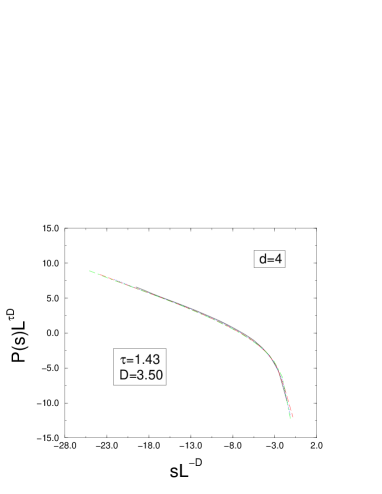
FIG. 1.: Data collapse analysis of the avalanche size distribution of the BTW model in $d=4$ with $\epsilon\equiv 0$ and for lattice sizes $L=48,80,112$ and $144$. The plot is on a double logarithmic scale.

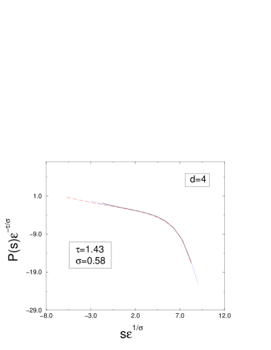
FIG. 2.: Data collapse analysis of the avalanche size distribution of the BTW model in $d=4$ with $L=144$ and for dissipation rates $\epsilon>10^{-1}$.The plot is on a double logarithmic scale.

REFERENCES

- [1] P. Bak, C. Tang and K. Wiesenfeld, Phys. Rev. Lett. 59, 381 (1987); Phys. Rev. A 38, 364 (1988).
- [2] For a review see: G. Grinstein, in Scale Invariance, Interfaces and Non-Equilibrium Dynamics, edited by A. McKane et al., NATO Advanced Study Institute, Series B: Physics Vol. 344 (Plenum, New York, 1995).
- [3] D. Sornette, A. Johansen and I. Dornic, J. Phys. I (France) 5 325 (1995).
- [4] A. Vespignani and S. Zapperi, Phys. Rev. Lett. 78, 4793 (1997); Phys. Rev. E XXXX (1998).
- [5] Sandpile models are driven by adding a single energy grain on a randomly chosen site, when no active sites are present. In this way, avalanches are instantaneous with respect to the driving timescale. Non-locality is thus implicitly enforced in computer simulations, where the evolution of a single site depends on the state of the entire system.
- [6] Theoretical approaches generally focus on the critical avalanche behavior and the scaling with respect to the external driving is not considered. Y. C. Zhang, Phys. Rev. Lett. 63, 470 (1989); A.Díaz-Guilera, Europhys.Lett. 26, 177 (1994); A. Vespignani, S. Zapperi and L. Pietronero, Phys. Rev. E 51, 1711 (1995); S. Zapperi, K. B. Lauritsen, and H. E. Stanley, Phys. Rev. Lett. 75, 4071 (1995).
- [7] D. Dhar, Phys. Rev. Lett.64, 1613 (1990).
- [8] V. B. Priezzhev, J. Stat. Phys. 74, 955 (1994).
- [9] P. Grassberger and S. S. Manna, J. Phys. (France) 51, 1077 (1990).
- [10] S. S. Manna, J. Stat. Phys. 59, 509 (1990); Physica A 179, 249 (1991).
- [11] A. Ben-Hur and O.Biham, Phys. Rev. E 53, R1317 (1996).
- [12] S. Lübeck and K.D. Usadel, Phys. Rev. E 55, 4095 (1997); S. Lübeck, Phys. Rev. E 56, 1590 (1997).
- [13] S. Lübeck and K.D. Usadel, Phys. Rev. E 56, 5138 (1997).
- [14] R.Dickman, A.Vespignani and S.Zapperi, Phys. Rev. E xx, xxx (1998); For an introductory review on systems with absorbing states see R. Dickman in Nonequilibrium statistical mechanics in one dimension, V.Privman ed., (Cambridge Press, 1996).
- [15] S.S. Manna, L.B. Kiss and J. Kertesz, J. Stat. Phys. 61, 923 (1990).
- [16] K. Christensen and Z. Olami, Phys. Rev. E 48, 3361 (1993).
- [17] The relation has been already obtained from numerical simulations [9, 10] and proved analytically in d=2 [7].
- [18] A. Chessa, E. Marinari, A. Vespignani and S. Zapperi, unpublished.
- [19] For information see the web-site: http://kalix.unica.it/