Nonequilibrium transport for crossed Luttinger liquids

Abstract

Transport through two one-dimensional interacting metals (Luttinger liquids) coupled together at a single point is analyzed. The dominant coupling mechanism is shown to be of electrostatic nature. Describing the voltage sources by boundary conditions then allows for the full solution of the transport problem. For weak Coulomb interactions, transport is unperturbed by the coupling. In contrast, for strong interactions, unusual nonlinear conductance laws characteristic for the correlated system can be observed.

The physics of one-dimensional (1D) conductors has received much attention lately, chiefly due to fabrication advances and the discovery of novel 1D materials such as carbon nanotubes [1]. From the theoretical point of view, these systems are of interest since Coulomb interactions invalidate the ubiquitous Fermi liquid description. The resulting state is often of Luttinger liquid (LL) [2, 3] type characterized by, e.g., spin-charge separation, suppression of the tunneling density of states, and interaction-dependent power laws in the transport behavior. However, so far the unambiguous experimental observation of LL behavior has been difficult to achieve.

In this paper, we study two correlated 1D metals coupled in a point-like manner (“crossed Luttinger liquids”). For the standard two-chain problem, where two Luttinger liquids are connected all along the conductors, the coupling normally destroys the LL phase [4]. In the case of a point-like coupling, however, the LL characteristics can survive and lead to the unusual transport features reported below. The most promising candidates for their experimental observation are carbon nanotubes. At not exceedingly low temperatures, metallic single-wall nanotubes exhibit LL behavior (with an additional flavor index) [5]. In a remarkable recent experiment, Tans et al. [6] were able to attach leads to a single nanotube. So far, transport measurements have been dominated by Coulomb charging effects due to rather large contact resistances between the leads and the nanotube, thereby masking any possible deviation from Fermi liquid theory. In the near future this problem might be overcome, and non-Fermi liquid laws should indeed emerge. Other realizations of crossed Luttinger liquids could be based on, e.g., 1D quantum wires in semiconductor heterostructures [7], or edge states in a fractional quantum Hall bar [8].

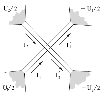
FIG. 1.: Two Luttinger liquids coupled together at one point ($x=0$) and connected to external reservoirs held at constant voltages $\pm U_{1}/2$ and $\pm U_{2}/2$. In the absence of single-particle tunneling, the currents obey $I_{i}=I_{i}^{\prime}$.

The geometry of our system is shown in Fig. 1. We shall consider two spinless Luttinger liquids characterized by the same interaction constant $g$ [9]. Here the noninteracting value is $g=1$, and externally screened Coulomb interactions imply $0<g<1$ [2, 3]. For the nanotube experiment of Ref.[6], one has an externally unscreened $e^{2}/|x-x^{\prime}|$ interaction potential and therefore very strong correlations. Strictly speaking, this interaction leads to $g\to 0$ in an infinite system, but the finite length of the nanotube in Ref.[6] implies $g\approx 0.2$. A natural and quite simple description of Luttinger liquids is offered by the standard bosonization method [3]. External reservoirs (voltage sources) can be incorporated by imposing boundary conditions [10] for the phase fields employed in the bosonization scheme. This approach offers a general and powerful route to studying multi-terminal Landauer-Büttiker geometries [11] for strongly correlated electrons. The crossed Luttinger liquids depicted in Fig. 1 may be the simplest example for such a problem.

We start by expressing the right- and left-moving ($p=\pm$) component of the electron operator $\psi_{pi}(x)$ in conductor $i=1$ or 2 in terms of the dual bosonic phase fields $\theta_{i}(x)$ and $\phi_{i}(x)$ obeying the algebra

$$[\phi_{i}(x),\theta_{j}(y)]_{-}=-(i/2)\delta_{ij}\,{\rm sgn}(x-y)\;.$$ (1)

The bosonization formula then reads [3]

$$\psi_{pi}(x)=\frac{\eta_{pi}}{\sqrt{2\pi a}}\exp[-ipk_{F}x-ip\sqrt{\pi g}\,\theta_{i}(x)-i\sqrt{\pi/g}\,\phi_{i}(x)]\;,$$ (2)

where the same average density $k_{F}/\pi$ is assumed for both conductors. The short-distance cutoff (lattice spacing) in Eq. (2) is taken as $a=1/k_{F}$. To ensure anticommutation relations among different branches $(p,i)$, we use (real) Majorana fermions $\eta_{pi}$ fulfilling $[\eta_{pi},\eta_{p^{\prime}i^{\prime}}]_{+}=2\delta_{pp^{\prime}}\delta_{ii^{\prime}}$. In the following, only products of Majorana fermions will appear. A valid choice for these products employs the standard Pauli matrices [5],

$$\eta_{p1}\eta_{p2}=i\sigma_{x}\;,\quad\eta_{p1}\eta_{-p,2}=-ip\sigma_{y}\;,$$ (3)

$$\eta_{p1}\eta_{-p1}=ip\sigma_{z}\;,\quad\eta_{p2}\eta_{-p2}=-ip\sigma_{z}\;.$$ (4)

Assuming that the conductors do not contain impurities, the Hamiltonian of the uncoupled system is

$$H_{0}=\frac{1}{2}\int dx\sum_{i=1,2}\left\{(\partial_{x}\phi_{i})^{2}+(\partial_{x}\theta_{i})^{2}\right\}\;,$$ (5)

where we have put $\hbar=1$ and the sound velocity $v=v_{F}/g=1$. Adiabatically connected voltage sources can then be taken into account by Sommerfeld-like boundary conditions. Applying the voltage $U_{1}$ along conductor 1, and $U_{2}$ along conductor 2, see Fig. 1, they read [10]

$$\langle\rho_{p=\pm,i}(x\to\mp\infty)\rangle=\pm\frac{eU_{i}}{4\pi g}\;,$$ (6)

where $\rho_{\pm,i}$ is the density of right/left-moving particles injected into conductor $i$. Outgoing particles are assumed to enter the reservoirs without reflection.

Let us now consider a point-like coupling of both 1D conductors at, say, $x=0$. For example, in a nanotube setup, two nanotubes could be stacked on top of each other. Such a contact causes (at least) two different coupling mechanisms [12].

First, there arises a (density-density) electrostatic interaction of the form $V_{1}=\lambda_{1}\rho_{1}(0)\rho_{2}(0)$. Using Eqs. (2) and (3), and omitting the mean density $k_{F}/\pi$ which is supposedly neutralized by positive background charges, the bosonized representation of the density operator is

$$\rho_{i}(x)=\sqrt{\frac{g}{\pi}}\,\partial_{x}\theta_{i}(x)\mp\frac{\sigma_{z}}{\pi a}\sin[2k_{F}x+\sqrt{4\pi g}\,\theta_{i}(x)]\;,$$ (7)

where the first (“slow”) term is due to the sum of right- and left-moving densities $\rho_{Ri}+\rho_{Li}$, and the second (“fast”) term arises from mixing right- and left-movers. The $\mp$ signs correspond to $i=1,2$, respectively. One checks easily that most contributions to $V_{1}$ are irrelevant for $g\leq 1$, i.e., they have scaling dimension $\eta>1$. Keeping the fast component in Eq. (7) yields the only important term,

$$V_{1}=-\frac{\lambda_{1}}{(\pi a)^{2}}\sin[\sqrt{4\pi g}\,\theta_{1}(0)]\sin[\sqrt{4\pi g}\,\theta_{2}(0)]\;,$$ (8)

with scaling dimension $\eta_{1}=2g$. Clearly, this coupling becomes relevant for sufficiently strong interactions, $g<1/2$. In contrast, a static potential scatterer in one of the conductors would be relevant already for $g<1$ [13]. In our case, electrons in conductor 1 experience the fluctuating potential scattering $V_{1}$ due to electrons in conductor 2, implying a doubled scaling dimension.

The second potentially important process is single-particle hopping from one conductor into the other. It is helpful to distinguish processes that do (do not) preserve the $p=R,L=\pm$ index, yielding the two perturbations $V_{2}=\lambda_{2}\sum_{p}\psi^{\dagger}_{p1}(0)\psi_{p2}(0)+$ H.c. (preserving the $p$ index) and $V_{3}=\lambda_{3}\sum_{p}\psi^{\dagger}_{p1}(0)\psi_{-p2}(0)+$ H.c. (not preserving the $p$ index). They have the bosonized form

$$V_{2} = -\frac{2\lambda_{2}}{\pi a}\sigma_{x}\cos\{\sqrt{\pi g}\,[\theta_{1}(0)-\theta_{2}(0)]\}$$ (10)

$$\quad\times\sin\{\sqrt{\pi/g}\,[\phi_{1}(0)-\phi_{2}(0)]\}$$

$$V_{3} = \frac{2\lambda_{3}}{\pi a}\sigma_{y}\sin\{\sqrt{\pi g}\,[\theta_{1}(0)+\theta_{2}(0)]\}$$ (12)

$$\quad\times\cos\{\sqrt{\pi/g}\,[\phi_{1}(0)-\phi_{2}(0)]\}\;.$$

For the standard two-chain problem, a (bulk) coupling term formally identical to Eq. (10) has been discussed in Ref.[14]. Both $V_{2}$ and $V_{3}$ have scaling dimension $\eta_{2}=\eta_{3}=(g+1/g)/2>1$, from which one might naively conclude that they are irrelevant [15]. However, this conclusion is premature because $V_{2}$ and $V_{3}$ have conformal spin $S=1$ [16]. For an operator with non-zero conformal spin, the standard criterion for relevance $\eta<1$ does not apply, since relevant perturbations may be generated in higher orders of the renormalization group (RG). This phenomenon indeed occurs in the standard two-chain problem [17], where the (bulk) coupling term corresponding to Eq. (10) generates relevant particle-hole and/or particle-particle excitation operators. Similarly, we find that $V_{2}$ and $V_{3}$ together generate the electrostatic coupling $V_{1}$ given in Eq. (8), but no other relevant terms. Omitting irrelevant operators, the resulting RG equations take the closed form

$$\frac{d\lambda}{d\ell} = [1-2g]\,\lambda+[g-1/g]\,t^{2}\;,$$ (13)

$$\frac{dt}{d\ell} = [1-(g+1/g)/2]\,t\;,$$ (14)

where $\lambda_{2}=\lambda_{3}\equiv t$ is the hopping amplitude and $\lambda_{1}\equiv\lambda$ the electrostatic coupling. The standard flow parameter is defined by $d\ell=-d\ln\omega_{c}$, where $\omega_{c}$ is a high-frequency cutoff that is reduced under the RG transformation.

Let us first discuss the case $g=1$. The electrostatic coupling is irrelevant, i.e., we may effectively put $\lambda=0$, but the hopping term stays marginal. By refermionizing the Hamiltonian $H_{0}+V_{2}+V_{3}$, and employing the boundary conditions (6), one arrives at the familiar results for uncorrelated electrons in the geometry of Fig. 1, see Ref. [11]. We therefore recover the usual Landauer-Büttiker formalism. Second, for $g<1$, the hopping amplitude $t(\ell)$ always scales to zero as $\ell\to\infty$, and the effects of single-particle tunneling can be captured by a renormalization of the bare electrostatic coupling $\lambda$, see Eq. (13). We shall assume henceforth that this renormalization has been carried out, and only the electrostatic interaction $V_{1}$ will be kept. In that case, the currents flowing through conductor $i=1$ or 2 satisfy $I_{i}=I_{i}^{\prime}$, see Fig. 1, and can be computed from the bosonized current operator [3]

$$I_{i}=e\sqrt{g/\pi}\,\partial_{t}\theta_{i}(x=0,t)\;.$$ (15)

For weak interactions, $1/2<g<1$, the electrostatic coupling $\lambda(\ell)$ also flows to zero as $\ell\to\infty$. In that case, at low energy scales, crossed Luttinger liquids are basically insensitive to the coupling considered here. At asymptotically low energy scales, the currents are then $I_{i}=(e^{2}/h)\,U_{i}$. The finite-temperature or low-voltage corrections due to the irrelevant operators $V_{i}$ can be computed by perturbation theory in the respective coupling strengths $\lambda_{i}$. Since the fluctuating potential scattering is irrelevant for $1/2<g<1$, the corrections due to $V_{2,3}$ are governed by the standard exponent $\alpha=(g+g^{-1}-2)/4$ for tunneling into a bulk LL [2, 3]. This is in contrast to a static potential scatterer, where tunneling into the end of a LL matters at low energy scales [13].

Directly at $g=1/2$, the operator $V_{1}$ is marginal, and straightforward refermionization yields

$$I_{i}=\frac{e^{2}}{h}\,\frac{1}{1+(\lambda/2\pi a)^{2}}\,U_{i}\;.$$ (16)

Each conductor exhibits a response only to the voltage applied to itself, with the conductance now explicitly depending on the electrostatic coupling strength $\lambda$.

For sufficiently strong interactions, $g<1/2$, the electrostatic coupling $\lambda(\ell)$ flows to strong coupling. To proceed, we switch to the linear combinations

$$\vartheta_{\pm}(x) = \{\theta_{1}(x)\pm\theta_{2}(x)\}/\sqrt{2}\;,$$ (17)

$$\varphi_{\pm}(x) = \{\phi_{1}(x)\pm\phi_{2}(x)\}/\sqrt{2}\;,$$ (18)

which again obey the algebra (1). Remarkably, the Hamiltonian $H_{0}+V_{1}$ decouples into the sum $H_{+}+H_{-}$ with

$$H_{\pm} = \frac{1}{2}\int dx\left\{(\partial_{x}\varphi_{\pm})^{2}+(\partial_{x}\vartheta_{\pm})^{2}\right\}$$ (20)

$$\quad\pm\frac{\lambda}{2(\pi a)^{2}}\cos\left[\sqrt{8\pi g}\,\vartheta_{\pm}(0)\right]\;,$$

and the boundary conditions (6) determining the density $\bar{\rho}_{p,r}$ of $p=\pm$ movers injected into channel $r=\pm$ take the form

$$\langle\bar{\rho}_{p,r}(x\to-p\infty)\rangle=\frac{p}{\sqrt{2}}\frac{e(U_{1}+rU_{2})}{4\pi g}\;.$$ (21)

Therefore we are left with two completely decoupled systems $r=\pm$, each of which is formally identical to the problem of an elastic potential scatterer embedded into a spinless LL [13]. However, this LL now has the doubled interaction strength parameter $\bar{g}=2g$. The boundary conditions (21) specify the effective voltages $\bar{U}_{r}=(U_{1}+rU_{2})/\sqrt{2}$ applied to channel $r=\pm$. In analogy to Eq. (15), currents in channel $r=\pm$ are defined by $\bar{I}_{r}=e\sqrt{g/\pi}\,\partial_{t}\vartheta_{r}(0)$, and from Eq. (17), we then find the currents $I_{i}=(\bar{I}_{+}\pm\bar{I}_{-})/\sqrt{2}$ flowing in conductor $i=1,2$.

The Hamiltonian (20) has been discussed in detail before, see, e.g., Refs.[13, 18, 19, 20, 21]. For arbitrary $\bar{g}$, the exact solution of the transport problem has been given in Ref.[19]. This solution exploits the integrability of Eq. (20) and employs the thermodynamic Bethe ansatz. Simpler exact solutions are possible by means of refermionization techniques for $\bar{g}=1$ [see Eq. (16)] and $\bar{g}=1/2$. The case $g=1/2$ thus corresponds to an uncorrelated situation in the new basis (17), and $g=1/4$ is the Toulouse point [20]. Progress can also be made by expanding in $|\epsilon|\ll 1$ for $\bar{g}=1-\epsilon$ [18] or $\bar{g}=1/2-\epsilon$ [21].

Employing the exact results of, e.g., Ref.[19], at zero temperature we find the asymptotic low-voltage behavior

$$I_{i} = \frac{e^{2}}{h}\frac{\lambda_{B}}{e}\,\Bigl{\{}\,{\rm sgn}(U_{1}+U_{2})\,[e|U_{1}+U_{2}|/\lambda_{B}]^{1/g-1}$$ (23)

$$\quad\pm\;{\rm sgn}(U_{1}-U_{2})\;[e|U_{1}-U_{2}|/\lambda_{B}]^{1/g-1}\Bigr{\}}\;,$$

where the $\pm$ sign corresponds to $i=1,2$, respectively. The energy scale $\lambda_{B}$ generated by the bare electrostatic coupling $\lambda$ is given by

$$\lambda_{B}=(c_{g}/a)\,(\lambda/a)^{1/[1-2g]}\;,$$ (24)

where $c_{g}$ is a numerical constant of order unity [19]. The result (23) holds under the condition

$$e|U_{1}\pm U_{2}|\ll\lambda_{B}\;.$$ (25)

If both voltages approach zero, the linear conductance vanishes in both 1D conductors. We thus find a pronounced zero-bias anomaly, with characteristic interaction-dependent power laws for small voltages.

Let us now discuss the full current-voltage characteristics. A particularly simple solution emerges at the Toulouse point $g=1/4$ by refermionization [20] of Eq. (20) under the boundary conditions (21). At zero temperature, the result is

$$\bar{I}_{\pm}=(e^{2}/h)\,[U_{\pm}-V_{\pm}]\;,$$ (26)

where $V_{\pm}$ is the four-terminal voltage [10] subject to the self-consistency equation

$$eV_{\pm}=2\lambda_{B}\tan^{-1}\{[2eU_{\pm}-(3/2)eV_{\pm}]/\lambda_{B}\}\;,$$ (27)

where $\lambda_{B}=\lambda^{2}/4(\pi a)^{3}$ in accordance with Eq. (24). Under the condition (25), the exact result (26) reproduces Eq. (23) again. In the absence of a coupling, $\lambda_{B}=0$, one finds the correct unperturbed currents $I_{i}=(e^{2}/h)U_{i}$.

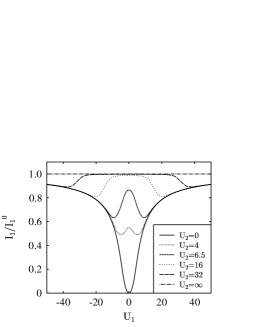
FIG. 2.: Transport current $I_{1}$ normalized to the unperturbed value $I_{1}^{0}=(e^{2}/h)\,U_{1}$ for $g=1/4,\lambda_{B}/e=1,T=0$, and several values of the cross voltage $U_{2}$.

The transport current $I_{1}$ is plotted as a function of $U_{1}$ in Fig. 2. Contrary to what is found in the uncorrelated system [11], the current $I_{1}$ is extremely sensitive to the applied cross voltage $U_{2}$. For $U_{2}=0$, transport becomes fully suppressed for $U_{1}\to 0$, with $g$-dependent nonlinear low-voltage corrections given by Eq. (23). Increasing $U_{2}$ for some fixed $U_{1}$ then leads to an increase in the current $I_{1}$. Eventually, the linear conductance behavior is restored for very large cross voltage. In fact, for $e|U_{1}\pm U_{2}|\gg\lambda_{B}$, one always recovers the unperturbed currents $I_{i}=(e^{2}/h)\,U_{i}$. The generic correlation effects are most important under the conditions (25).

Remarkably, there is a suppression of the current if $U_{1}=\pm U_{2}$, which is observed as a “dip” in the normalized current displayed in Fig. 2. This effect can be rationalized in terms of a partial dynamical pinning of charge density waves in conductor 1 due to commensurate charge density waves in conductor 2. As can be checked from Eq. (26), while the nonlinear conductance $G_{11}\equiv\partial I_{1}/\partial U_{1}$ stays positive, one can have a negative value for $G_{12}\equiv\partial I_{1}/\partial U_{2}$. In fact, the latter (off-diagonal) conductance is within the bounds $-e^{2}/2h\leq G_{12}\leq e^{2}/2h$ [we note that $G_{12}=0$ for $g\geq 1/2$], while the diagonal conductance fulfills $0\leq G_{11}\leq e^{2}/h$. The pronounced and nonlinear sensitivity of the current $I_{1}$ to the applied cross voltage $U_{2}$ is a distinct fingerprint for Luttinger liquid behavior. Parenthetically, anomalous power laws can also be found in the temperature dependence of the current.

To conclude, we have examined nonlinear transport through two Luttinger liquids coupled together at one point. The only relevant coupling is of electrostatic origin and leads to distinct correlation effects for strong Coulomb interactions, $g<1/2$. The theoretical findings reported here could be of use for the experimental identification of non-Fermi-liquid behavior in carbon nanotubes and other one-dimensional materials.

We thank A.O. Gogolin, H. Grabert, and C.A. Stafford for useful discussions. This work was supported by the Deutsche Forschungsgemeinschaft (Bonn).

REFERENCES

- [1] S. Iijima, Nature 354, 56 (1991); A. Thess et al., Science 273, 483 (1996).
- [2] J. Voit, Rep. Prog. Phys. 57, 977 (1995).
- [3] A.O. Gogolin, A.A. Nersesyan, and A.M. Tsvelik, Bosonization and Strongly Correlated Systems (Cambridge University Press, 1998).
- [4] See, e.g., M. Fabrizio, Phys. Rev. B 48, 15 838 (1993).
- [5] R. Egger and A.O. Gogolin, Phys. Rev. Lett. 79, 5082 (1997).
- [6] S.J. Tans, M.H. Devoret, H. Dai, A. Thess, R.E. Smalley, L.J. Geerligs, and C. Dekker, Nature 386, 474 (1997).
- [7] A.O. Gogolin, Ann. Phys. (Paris) 19, 411 (1994).
- [8] Tunneling from three chiral Luttinger liquids onto a dot is treated by C. Nayak, M.P.A. Fisher, A.W.W. Ludwig, and H.-H. Lin, preprint cond-mat/9710305.
- [9] The same effects as discussed here for spinless electrons are also found for spin- electrons or in carbon nanotubes. The minor modifications required in these two cases and the extension to different parameters for both conductors will be presented elsewhere.
- [10] R. Egger and H. Grabert, Phys. Rev. Lett. 77, 538 (1996).
- [11] S. Datta, Electronic Transport in Mesoscopic Systems, Chapter 2 (Cambridge University Press, 1995).
- [12] If the conductors are brought into mechanical contact, local deformations might cause impurity scattering in one or both conductors. For simplicity, we assume that no such impurity scattering processes are present.
- [13] C.L. Kane and M.P.A. Fisher, Phys. Rev. B 46, 15 233 (1992).
- [14] F.V. Kusmartsev, A. Luther, and A.A. Nersesyan, JETP Lett. 55, 724 (1992).
- [15] For a bulk coupling such as in Refs.[4, 14], a perturbation is relevant already for .
- [16] If the operators and are taken in a strictly local sense, the concept of non-zero conformal spin does not apply and both operators are simply irrelevant. In practice, however, they might act over some finite (but small) distance around . Thereby one generates the second-order contribution in Eq. (13).
- [17] V.M. Yakovenko, JETP Lett. 56, 510 (1992).
- [18] D. Yue, L.I. Glazman, and K.A. Matveev, Phys. Rev. B 49, 1966 (1994).
- [19] P. Fendley, A.W.W. Ludwig, and H. Saleur, Phys. Rev. B 52, 8934 (1995).
- [20] F. Guinea, Phys. Rev. B 32, 7518 (1985); C. de C. Chamon, D.E. Freed, and X. Wen, ibid. 53, 4033 (1996).
- [21] U. Weiss, R. Egger, and M. Sassetti, Phys. Rev. B 52, 16 707 (1995); U. Weiss, Solid State Comm. 100, 281 (1996).