Van der Waals interaction between flux lines in High-$T_{c}$ Superconductors

Abstract

In anisotropic or layered superconductors thermal fluctuations as well as impurities induce a van der Waals (vdW) attraction between flux lines, as has recently been shown by Blatter and Geshkenbein in the thermal case [Phys. Rev. Lett. 77, 4958 (1996)] and by Mukherji and Nattermann in the disorder dominated case [Phys. Rev. Lett. 79, 139 (1997)]. This attraction together with the entropic or disorder induced repulsion has interesting consequences for the low field phase diagram. We present two derivations of the vdW attraction, one of which is based on an intuitive picture, the other one following from a systematic expansion of the free energy of two interacting flux lines. Both the thermal and the disorder dominated case are considered. In the thermal case in the absence of disorder, we use scaling arguments as well as a functional renormalization of the vortex-vortex interaction energy to calculate the effective Gibbs free energy on the scale of the mean flux line distance. We discuss the resulting low field phase diagram and make quantitative predictions for pure BiSCCO (Bi₂Sr₂CaCu₂O₈). In the case with impurities, the Gibbs free energy is calculated on the basis of scaling arguments, allowing for a semi-quantitative discussion of the low-field, low-temperature phase diagram in the presence of impurities.

1 Introduction

Conventional type–II superconductors show in addition to the flux repulsing Meissner state a second superconducting (Abrikosov) phase in which the magnetic induction ${\bf B}$ enters the material in the form of quantized flux lines (FLs) which form a triangular lattice. Each FL carries a unit flux quantum $\Phi_{0}=hc/2e$. The Abrikosov lattice is characterized by a non–zero shear modulus $c_{66}$, which vanishes at the upper and lower critical field, $H_{c_{2}}$ and $H_{c_{1}}$, where continuous transitions to the normal and the Meissner state, respectively, occur. In his mean–field solution Abrikosov treats FLs as stiff rods. Close to the lower critical field $H_{c_{1}}$, their interaction becomes exponentially weak and hence the FL density $\ell^{-2}=B/\Phi_{0}$ vanishes as $|\ln\tilde{h}|^{-2}$ where $\tilde{h}=(H-H_{c_{1}})/H_{c_{1}}$ denotes the reduced field strength tink .

Thermal fluctuations roughen the FLs resulting in a possible melting of the Abrikosov lattice close to $H_{c_{1}}$ and $H_{c_{2}}$, respectively, because of the softening of $c_{66}$. This applies in particular to high–$T_{c}$ materials with their elevated transition temperatures and their pronounced layer structures blatrev . At present, it is not clear whether the transition to the normal phase at high field happens in these materials via one or two transitions. However, melting of the FL lattice has clearly been observed experimentally gammel .

At low fields a first order melting transition to a liquid phase and a change in the critical behavior of $B$ has been predicted some time ago by NelsonNelson . Quantitatively the influence of thermal fluctuations is described by a thermal length scale $L_{T}=\Phi_{0}^{2}/(16\pi^{2}T)\approx 2\,{\rm cm}\,{\rm K}/T$ fish . $L_{T}$ has a simple physical meaning: an isolated flux line segment of length $L_{T}$ shows a thermal mean square displacement of the order of the London penetration length $\lambda$. Besides a shift of $H_{c_{1}}$, large scale thermal fluctuations lead close to $H_{c_{1}}$ to an entropic repulsion $\sim(\lambda^{2}/L_{T}\ell)^{2}$ between FLs which dominates over the bare interaction for small $\tilde{h}$ and hence $B\sim\tilde{h}$ Nelson . Here and below, all FL interactions are measured in units of $\varepsilon_{\circ}=(\Phi_{0}/4\pi\lambda)^{2}=L_{T}T/{\lambda}^{2}$.

More recently, Blatter and Geshkenbein BlatterGeshkenbein found that in anisotropic or layered superconductors short scale fluctuations give rise also to an attractive van der Waals (vdW) interaction brandt . For FLs separated by a distance $R$ the strength of this interaction is of the order $-\lambda^{6}/(dL_{T}R^{4})$ for $\lambda<R<d/\varepsilon$ and of the order $-\lambda^{6}/(\varepsilon L_{T}R^{5})$ for $d/\varepsilon<R<\lambda/\varepsilon$. $\varepsilon^{2}=m/M\ll 1$ denotes the anisotropy of the material with $m$ and $M$ the effective masses parallel and perpendicular to the $ab$ plane, and $d$ the interlayer spacing. $\lambda$ and $\lambda/\varepsilon$ are then the screening lengths parallel and perpendicular to the layers, respectively.

The competition among the bare, the entropic and the vdW interactions leads to an interesting phase diagram at low $B$ values. In particular, Blatter and Geshkenbein BlatterGeshkenbein find at low $T$ a first order transition between the Meissner and the Abrikosov phase.

So far fluctuation effects have been discussed for a clean superconductor. It is well known, however, that in type–II superconductors FLs must be pinned in order to prevent dissipation from their motion under the influence of an external current. Therefore, besides the thermal fluctuations one has to take into account the effect of disorder. Randomly distributed pinning centers lead indeed to a destruction of the Abrikosov lattice larkin , but as has been recently shown, for not too strong disorder FLs may form a (Bragg–) glass phase which is characterized by quasi long–range order of the FL lattice bragg . For low $B$ this phase undergoes a melting transition to a pinned liquid state. Inside this phase, disorder induced effects are expected to dominate over those of thermal fluctuations for sufficiently low $T$. The influence of the disorder fluctuation induced forces between the FLs and the consequences for the low $B$ phase diagram – which deviates substantially from that found in Ref. BlatterGeshkenbein for pure systems – have been considered in NattermannMukherji .

In this paper, we address several issues. We start with a review of the interactions between FLs and the derivation of the properties of an isolated FL in section 2. Correlation functions, both in the thermal and in the disordered case, are calculated. These are needed for the calculation of the van der Waals interaction in section 3. There, we first develop an intuitive picture to derive the vdW energy driven by thermal fluctuations and by disorder. In the presence of strong disorder, detailed level statistics of the random impurity distribution are necessary. In the second part of this section, a thorough derivation of the van der Waals interaction by a systematic expansion of the free energy of two fluctuating FLs BlatterGeshkenbein ; NattermannMukherji is presented.

The consequences for the low field phase diagram of anisotropic high-$T_{c}$ superconductors are considered in section 4. In the thermal case, a functional renormalization group is used to calculate the effective Gibbs free energy on the scale of the mean distance $\ell$ between FLs. In particular, the bare interaction between flux lines, which is given by the superposition of the bare repulsion and the vdW attraction, is renormalized by integrating out thermal fluctuations on scales between $\lambda$ and $\ell$. The results of this calculation are compared to an expression for the Gibbs free energy based on scaling arguments. In this latter approach, the contribution from the vdW interaction can be estimated only up a to numerical factor determining its amplitude; this factor will be quantified using the results from the renormalization procedure. In the case with disorder, we give an expression for the Gibbs free energy that is based on scaling arguments, and which allows for a semi-quantitative discussion for the low-field, low-temperature phase diagram in the presence of impurities.

2 Single chain properties

In this section we discuss properties of an isolated flux line (FL). Starting with a vortex lattice picture with the general form of the interaction between the FLs, we consider the limit of a very dilute lattice where a single chain approximation is good enough. A single FL in the dilute limit is well described by a dispersive stiffness constant $\varepsilon_{l}(k_{z})$, the origin and different limiting properties of which are discussed. Deriving the Hamiltonian for a FL in an isotropic material, we generalize it for a FL in the presence of impurities with its full dispersive stiffness constant. Finally, we discuss the properties of several correlation functions in the presence of impurities. These correlation functions will be used in the derivation of the van der Waals interaction in section 3.

2.1 Interactions and elastic constants

In reality the flux lines are not straight; they are distorted from their equilibrium positions. The displacement with respect to the equilibrium position ${\bf r}_{i}\equiv({\bf a}_{i},z)$, where $i$ denotes a site on the planar lattice, is represented by a two dimensional vector ${\bf u}_{i}(z)$ blatrev . In the low field limit, where the London theory is applicable, the interaction energy between $N$ vortices is in general given by

$${\cal F}=\frac{\varepsilon_{\circ}}{2}\sum_{i,j=1}^{N}\int d{s}_{i\alpha}\ d{s}_{j\beta}\ V^{\rm int}_{\alpha\beta}({\bf s}_{i}-{\bf s}_{j}),$$ (1)

where ${\bf s}_{i}={\bf r}_{i}+{\bf u}_{i}(z)$ is the position vector of the distorted vortex segment. $(\alpha\beta)\in(x,y,z)$ indicate different components. In (1) the terms with $i=j$ have been included. These terms correspond to the interaction between the segments of the same vortex line and therefore contribute to the self energy of the line. In isotropic materials the interaction is exponentially damped and is of the form ${e^{-r/\lambda}}/{r}$ with a short distance cutoff at the coherence length $r=\xi$. The high temperature oxide superconductors are essentially layered with the conducting CuO planes parallel to the $ab$ plane. A large anisotropy between the $c$ axis and the $ab$ plane due to this layered structure leads to many unusual properties compared to the isotropic materials.

The tensorial London potential between the vortices is conventionally expressed through its Fourier transform defined as $V^{\rm int}_{\alpha\beta}({\bf r})=4\pi\lambda^{2}\int d^{3}k/(2\pi)^{3}\,e^{i{\bf kr}}{\tilde{V}}^{\rm int}_{\alpha\beta}({\bf k})$ brandt3 . In our case, however, it turns out to be more convenient to express it in terms of its partial Fourier transform with respect to the $z$-direction only, as defined by

$$V_{\alpha\beta}^{\rm int}({\bf R},k_{z})=\frac{1}{4\pi\lambda^{2}}\int dz\;e^{-ik_{z}z}\,V_{\alpha\beta}({\bf R},z),$$ (2)

where ${\bf r}=({\bf R},z)$. This choice has the advantage of an explicit dependence on the distance ${\bf R}$ between FLs. Choosing ${\bf R}=(R,0)$ and $R\gtrsim\lambda$, the only contributions to the tensorial London potential that do not vanish by symmetry are

$$V_{zz}^{\rm int}({\bf R},k_{z})=-\frac{1}{2\pi\lambda^{2}}\;K_{0}\left(\sqrt{1+\lambda^{2}k_{z}^{2}}\,R/\lambda\right)$$ (3)

and

$$V_{xx}^{\rm int}({\bf R},k_{z})=-V_{yy}^{\rm int}({\bf R},k_{z})$$ (4)

$$\qquad=-\frac{1}{2\pi R}\frac{\varepsilon}{\lambda\sqrt{1+\lambda^{2}k_{z}^{2}}}\,K_{1}\left(\varepsilon\sqrt{1+\lambda^{2}k_{z}^{2}}\,R/\lambda\right).$$

$K_{n}(x)$ is the modified Bessel function of the second kind of $n^{\rm th}$ order. In the extreme anisotropy limit $\varepsilon\rightarrow 0$, this latter equation (4) simplifies to

$$V_{xx}^{\rm int}({\bf R},k_{z})=-\frac{1}{2\pi\,R^{2}}\,\frac{1}{1+\lambda^{2}k_{z}^{2}}.$$ (5)

In (3) to (5), a short distance cutoff at the coherence length $\xi$ is implied. In (4) and (5) subdominant terms of order $e^{-R/\lambda}$ have been neglected.

Different elastic moduli of the vortex lattice can be obtained from (1) by expanding in small displacement ${\bf u}$. For very small field $H\lesssim H_{c_{1}}$, the shear and compression moduli $c_{66}$ and $c_{11}(k)$ decay exponentially with the lattice spacing $\ell$ and can be neglected in a very dilute limit. The tilt modulus $c_{44}(k)$ is only weakly dispersive in isotropic materials brandt4 . In anisotropic materials, though, it has a much stronger dispersivity brandt1 ; blatrev which results, in the single FL limit, in a strongly dispersive elastic stiffness constant $\varepsilon_{l}(k_{z})=\ell^{2}c^{c}_{44}(k_{z})$ consisting of two parts,

$$\varepsilon_{l}(k_{z})\approx\frac{\varepsilon^{2}\varepsilon_{\circ}}{2}\ln\left(\frac{\kappa_{c}^{2}}{1+\lambda^{2}k_{z}^{2}}\right)+\frac{\varepsilon_{\circ}}{2\lambda^{2}k_{z}^{2}}\ln(1+k_{z}^{2}\lambda^{2}),$$ (6)

where $\kappa_{c}=\kappa/\varepsilon$ with the Ginzburg-Landau parameter $\kappa=\lambda/\xi$. $c^{c}_{44}(k_{z})$ is the part of the tilt modulus that originates from the self-energy of the vortices. The first part in (6) represents the Josephson coupling between the layers and is absent in the limit $\varepsilon\rightarrow 0$. The second part describes the contribution from the electromagnetic coupling, which remains finite in this limit. In the extreme short wavelength regime $\lambda k_{z}>1/\varepsilon$ the contribution due to the Josephson coupling dominates over the electromagnetic part and the line stiffness is given by the first term in (6). In the intermediate regime $1/\lambda<k_{z}<1/\varepsilon\lambda$, the electromagnetic interaction dominates, and the elastic constant is given by the second term in (6), hence the stiffness is highly dispersive in this regime. In the long wavelength limit, the line stiffness reaches a constant,

$$\varepsilon_{l}(k_{z})\approx\frac{\varepsilon_{\circ}}{2}\,(1+\varepsilon^{2}\ln\kappa_{c}^{2})\qquad\mbox{for }\lambda k_{z}\ll 1.$$ (7)

In order to obtain an estimate for the contributions from the Josephson and the electromagnetic coupling to the stiffness constant at small length scales we use $k_{z}=\pi/d$, where the layer spacing $d$ is the lowest relevant length scale. Using the parameters $\lambda=2000\,$Å, $\xi=20\,$Å, $d=15\,$Å and $\varepsilon=1/300$ blatrev , suitable for BiSCCO (Bi₂Sr₂CaCu₂O₈), we find that the contributions from the electromagnetic and the Josephson couplings are about equal in magnitude at this wavelength, while for lower $k_{z}$, the electromagnetic part dominates. Hence, for BiSCCO the Josephson coupling may be entirely neglected. For materials with a larger value of $\varepsilon$, on the other hand, $k_{z}=\pi/d$ belongs to the extreme short wavelength limit ($\lambda k_{z}>1/\varepsilon$) where the weakly dispersive Josephson coupling dominates.

2.2 Hamiltonian for a single Flux line

The line stiffness $\varepsilon_{l}(k_{z})$ obtained above can be used to describe FLs as elastic strings with a strongly dispersive elastic constant. In practice it is difficult to predict the properties of the FL at all wavelengths. Often in the following we therefore aim at large or small wavelength features depending on our interest in distortions on scales larger or smaller compared to $\lambda$. In the extreme long wavelength case where FLs are elastic strings with a dispersionless stiffness constant, the underlying lattice structure can be ignored. In the opposite limit the layered structure and the anisotropy become important blatrev . Depending on the ratio $\tau_{c}=2\xi_{c}^{2}/d^{2}$, where $\xi_{c}=\varepsilon\xi$ is the coherence length in the direction parallel to the $c$ axis with $\varepsilon$ denoting the anisotropy parameter, one can distinguish two cases, the continuous anisotropic limit and the extreme decoupled discrete limit. For $\tau_{c}\gg 1$ the coherence length is large enough to neglect the discrete layered structure. In that case the continuous anisotropic Ginzburg-Landau description is applicable. $\tau_{c}\ll 1$ is the decoupled limit where the Lawrence-Doniach model lawrence is more appropriate. In the latter case, instead of the continuous description, the vortex is often viewed as a stack of pancake vortices residing in layers but interconnected by Josephson strings between two successive CuO planes, as sketched in Fig. 1. The effect of the thermal energy or of random impurities is to displace the pancakes from their aligned position. Due to the dispersion these local displacements and their correlations will be different from the long wavelength distortions. It is however important to point out that the continuous anisotropic Ginzburg-Landau theory often provides a good description of the layered structure brandt2 unless specific thermodynamic properties, where the 2d structure is more important than the 3d bulk material, are investigated.

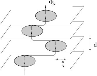
Figure 1: A single vortex line, carrying the flux $\Phi_{0}$, in a strongly layered superconductor. The flux line consists of an array of pancake vortices threading the individual superconducting layers which are separated by a distance $d$; the pancakes are interconnected by Josephson strings.

Taking into account the dispersivity of the stiffness constant of the FL, the Hamiltonian for a single FL in the presence of random impurities can be defined as

$${\cal H}(\{{\bf u}\})=\sum_{k}\ \frac{\varepsilon_{l}(k)}{2}\,k^{2}\,\tilde{{\bf u}}_{k}\tilde{{\bf u}}_{-k}+\int_{0}^{L}dz\,\varepsilon_{\rm pin}({\bf u}(z),z).$$ (8)

Here only the bending energy part has been expressed in momentum space with the Fourier transform of ${\bf u}(z)$ defined as

$${\tilde{\bf u}}_{k}=\frac{1}{\sqrt{L}}\int_{0}^{L}dz\ e^{ikz}{\bf u}(z).$$ (9)

Here and below, $k$ denotes the $k_{z}$-component of the full wave vector ${\bf k}$.

The random pinning potential is assumed to be Gaussian distributed with $\overline{\varepsilon_{\rm pin}(\bf u)}=0$ (a nonzero mean value $\overline{\varepsilon_{\rm pin}}$ simply shifts the Hamiltonian by a constant and is hence inconsequential) and

$$\overline{\varepsilon_{\rm pin}({\bf u},z)\varepsilon_{\rm pin}({\bf 0},0)}\;=\;\frac{T^{3}_{\rm dis}}{\varepsilon_{\circ}{\xi^{2}}}\;\delta(z)\tilde{k}({\bf u}/\xi)$$ (10)

with $\tilde{k}(x)=1$ for $x\ll 1$ and $\tilde{k}(x)\approx(1/x^{2})\ln x$ for $x\gg 1$, respectively blatrev . The overbar denotes the average over the disorder distribution. The displacement caused by the quenched disorder is strongly suppressed due to thermal smoothening for $T>T_{\rm dis}$. The characteristic energy $T_{\rm dis}$ can be related to the local shift in the critical temperature $T_{c}$ which is induced by an oxygen impurity density $n_{i}$ by

$$\frac{T_{\rm dis}^{3}}{(\varepsilon_{\circ}\xi)^{3}}=0.4\left(\frac{n_{i}}{T_{c}}\frac{dT_{c}}{dn_{i}}\right)^{2}\frac{1}{\xi^{3}n_{i}}\frac{1}{(1-t)^{1/2}},$$ (11)

where $t=T/T_{c}$ fish ; blatrev . This result holds in the case of non-optimal doping where $dT_{c}/dn_{i}\neq 0$; if this derivative vanishes, $T_{\rm dis}$ can be similarly related to the second derivative $d^{2}T_{c}/dn_{i}^{2}$ blatrev .

Statistical mechanics of a single FL in a random potential shows that the disorder is always relevant for $d\leq 2$. This is reflected through an enhanced averaged FL wandering on large scales $L>L_{\rm dis}$

$$\overline{\langle\,[\,{\bf u}(L)-{\bf u}(0)\,]^{2}\,\rangle}\sim\lambda(L/L_{\rm dis})^{\zeta}$$ (12)

with $\zeta>1/2$ for $d\leq 5$ kinzel . Here and in the following the angular bracket indicates thermal average. Several exact treatments at $d=2$ lead to $\zeta=2/3$. Disorder is marginally relevant at $d=3$. Numerical simulations and recent analytical calculations show $\zeta=5/8$ tang ; lassig . In the presence of disorder vortex segments of length $L_{\rm dis}$ are independently pinned. At $T=0$, this can be seen by minimizing the energy consisting of elastic and pinning contributions. Here the pinning energy is estimated within perturbation theory. This provides

$$L_{\rm dis}=\varepsilon_{\circ}\lambda^{2}\kappa^{1/\zeta-2}/T_{\rm dis}.$$ (13)

For $T<T_{\rm dis}$, the thermal fluctuations can be ignored and the above estimate of $L_{\rm dis}$ is still valid. For $T>T_{\rm dis}$, on the other hand,

$$L_{\rm dis}(T)=\frac{\varepsilon_{\circ}\xi^{2}}{T}\exp\left[\left(T/T_{\rm dis}\right)^{3}\right]$$ (14)

shows an exponential growth with the temperature as a consequence of the marginal relevance of the disorder at 3 space dimension NelsonDoussal . In the pure thermal case $\zeta=1/2$, and $L_{\rm dis}$ is replaced by fish

$$L_{T}=\varepsilon_{\circ}\lambda^{2}/T\;.$$ (15)

2.3 Correlation functions

With the ideas sketched above we now study several correlation functions in the presence of quenched impurities. Whereas in a pure system $\langle{\bf u}_{k}\rangle=0$ and hence $\langle{\bf u}_{k}{\bf u}_{-k}\rangle$ is the appropriate correlation function, in a random system one has to distinguish between the connected correlation function

$$C_{T}(k)={\overline{\langle{\bf u}_{k}{\bf u}_{-k}\rangle}}-{\overline{\langle{\bf u}_{k}\rangle\langle{\bf u}_{-k}\rangle}}$$ (16)

and the disconnected correlation function

$$C_{\rm dis}(k)={\overline{\langle{\bf u}_{k}\rangle\langle{\bf u}_{-k}\rangle}}.$$ (17)

We first study $C_{\rm dis}(k)$ and near the end of this section we show that the disorder does not affect $C_{T}(k)$ obtained in the pure case.

2.3.1 Short wavelength limit of $C_{\rm dis}(k)$

We first consider the short wavelength behavior of $C_{\rm dis}(k)$. In this limit the problem essentially simplifies to obtaining the typical displacement of a single pancake. A perturbative technique and an Imry-Ma type argument are applied to estimate the single pancake displacement.

As mentioned above in section 2.1, for highly anisotropic superconductors with very small values of $\varepsilon\ll 1$ (such as BiSCCO), the highest relevant wave vector $\pi/d$ is smaller than $1/\lambda\varepsilon$, with the consequence that in the short wavelength limit $\lambda k\gg 1$ it is sufficient to consider the dispersive elastic constant $\varepsilon_{l}(k)=(\varepsilon_{\circ}/\lambda^{2}k^{2})\ln(\lambda k)$. This term represents the contribution from the electromagnetic coupling in the full expression (6) for the line stiffness. A closer look at the elastic energy term in (8) with the dispersive elastic constant reveals that, apart from a logarithmic factor, the pancakes on different layers are essentially uncoupled. Thus rewriting the correlation function in real space

$${\overline{\langle{\bf u}_{k}\rangle\langle{\bf u}_{-k}\rangle}}=\frac{1}{L}\int dz\ dz^{\prime}e^{-ik(z-z^{\prime})}\overline{\langle{\bf u}(z)\rangle\langle{\bf u}(z^{\prime})\rangle},$$ (18)

we utilize the above assumption of independent pancake displacement, i.e.

$$\overline{\langle{\bf u}(z)\rangle\langle{\bf u}(z^{\prime})\rangle}=u_{\rm pv}^{2}f(z-z^{\prime}),$$ (19)

where

$$f(z)=\left\{\begin{array}[]{cl}1&\mbox{ for }|z|<d/2\\ \rule{0.0pt}{12.91663pt}0&\mbox{ for }d/2<|z|\ll\lambda.\end{array}\right.$$ (21)

This leads to

$$C_{\rm dis}(k)\approx{\overline{\langle u_{\rm pv}^{2}\rangle}}\,d\qquad\mbox{for}\quad 1\ll\lambda k\lesssim\pi\lambda/d.$$ (22)

The mean square displacement of a pancake in the presence of quenched impurities can be obtained from the Hamiltonian (8) which is, in the short wavelength limit, a superposition of the following two parts: (i) a parabolic elastic potential, $E_{\rm el}(u)\approx(u^{2}d/2)\,k^{2}\varepsilon_{l}(k)|_{k=\pi/d}$, which in the case considered here (where the electromagnetic coupling dominates) reads

$$E_{\rm el}(u)=\frac{1}{2}\frac{\varepsilon_{\circ}d}{\kappa^{2}}\ln(\pi\lambda/d)\frac{u^{2}}{\xi^{2}},$$ (23)

and (ii) a contribution from the disorder, averaged over the pancake height $d$,

$$\varepsilon_{\rm pin}({\bf u})\equiv\int_{0}^{d}dz\ \varepsilon_{\rm pin}({\bf r}+{\bf u}(z),z),$$ (24)

where ${\bf r}$ is the equilibrium position of the pancake.

It is useful to re-express this Hamiltonian in dimensionless variables $t=z/d$ and $\hat{\bf u}={\bf u}/\xi$. In terms of these dimensionless variables,

$$\frac{{\cal H}}{T} \approx \frac{\varepsilon_{\circ}d}{T\kappa^{2}}\ln(\pi\lambda/d)\,\times$$

$$\left\{\frac{\hat{\bf u}^{2}}{2}+\Delta^{1/2}(\pi\lambda/d)\int_{0}^{1}\!\!\!dt\ \tilde{\varepsilon}_{\rm pin}(\hat{\bf u},t)\right\},$$

where ${\tilde{\varepsilon}}_{\rm pin}(\hat{\bf u},t)$ is the pinning potential scaled to have a variance equal to unity, and we have defined

$$\Delta(x)=\Delta_{0}\,\frac{x}{\ln^{2}(1+x^{2})},\qquad\Delta_{0}=\left(\frac{T_{\rm dis}\kappa^{2}}{\varepsilon_{\circ}\lambda}\right)^{3}.$$ (26)

From (2.3.1) one concludes that in general, at finite temperature and finite disorder strength,

$${\overline{\langle u^{2}_{\rm pv}\rangle}}=\xi^{2}\Phi\left(\Delta(\pi\lambda/d),\;\frac{Td}{\xi^{2}\varepsilon_{l}(\pi/d)}\right),$$ (27)

where and $\Phi$ is a function of dimensionless variables for the disorder and the temperature.

In the absence of disorder ($\Delta_{0}=0$) fluctuations are driven by thermal energy and we have

$$\frac{\langle u^{2}_{\rm pv}\rangle_{\rm th}}{\xi^{2}}=\frac{2T}{\varepsilon_{\circ}d}\,\frac{\kappa^{2}}{\ln(\pi\lambda/d)}.$$ (28)

At $T=0$ and finite disorder $(T_{\rm dis}>0)$, the FL fluctuates to take advantage of the impurities, and the ground state displacement in this case is

$${\overline{u_{\rm pv}^{2}}}/{\xi^{2}}=F(\Delta(\pi\lambda/d))\equiv\Phi(\Delta(\pi\lambda/d),0).$$ (29)

For very low temperatures $T\ll T_{\rm dis}$, we can approximate the mean square displacement as

$$\overline{\langle{\bf u}_{\rm pv}^{2}\rangle}\approx\overline{{\bf u}_{\rm pv}^{2}}=\xi^{2}F(\Delta(\pi\lambda/d)).$$ (30)

In order to determine the explicit functional form of $F(\Delta)$, we take a recourse to a perturbative approach valid for small displacements $u\ll\xi$. In order to go beyond the perturbative regime, an Imry-Ma type scaling argument and the result from numerical simulations are discussed. In general we expect a power law form of

$$F(\Delta)\sim\Delta^{\eta}$$ (31)

and we attempt to get the value of $\eta$.

In the perturbative scheme we proceed with the reduced Hamiltonian (2.3.1) for a single pancake vortex. Expansion of the pinning energy in small displacement $\hat{\bf u}$

$$\tilde{\varepsilon}_{\rm pin}(\hat{\bf u},t)=\tilde{\varepsilon}_{\rm pin}(0,t)+\hat{\bf u}\cdot\nabla\tilde{\varepsilon}_{\rm pin}(\hat{\bf u},t)\big{|}_{\hat{\bf u}=0}+\ldots$$ (32)

and minimization of the total energy with respect to the displacement leads to the force equation

$$\hat{\bf u}=-\Delta^{1/2}(\pi\lambda/d)\int_{0}^{1}dt\,\nabla\tilde{\varepsilon}_{\rm pin}(\hat{\bf u},t)\big{|}_{\hat{\bf u}=0}\;.$$ (33)

Averaging over the dimensionless distribution $\tilde{\varepsilon}_{\rm pin}(\hat{\bf u},t)$ directly leads to the disorder induced short length scale displacement

$$\overline{u_{\rm pv}^{2}}\simeq\xi^{2}\Delta(\pi\lambda/d).$$ (34)

Thus, within the perturbative approach $\eta=1$.

Due to the narrow range of applicability of the perturbation technique, a more general nonperturbative scheme is needed for $\Delta(\pi\lambda/d)\gg 1$. This can be done by an Imry-Ma or variational approach engel , which briefly proceeds as follows. Consider the dimensionless part (in curly brackets) of the single pancake Hamiltonian (2.3.1). The displacement of a single pancake by an amount $\hat{\bf u}$ is associated with the elastic energy cost $\hat{\bf u}^{2}/2$. This energy cost has to be compared with the possible gain in pinning energy corresponding to the adjustment of the pancake position to a minimum of the random potential within the area $\pi\hat{\bf u}^{2}$. This energy is obtained from the second term in (2.3.1) and is of order $\Delta^{1/2}(\pi\lambda/d)$, where we have used that $\tilde{\varepsilon}(\hat{\bf u},t)$ has been scaled to unity, i.e.

$$\overline{\int_{0}^{1}dt\,\tilde{\varepsilon}_{\rm pin}(\hat{\bf u},t)\int_{0}^{1}dt^{\prime}\,\tilde{\varepsilon}_{\rm pin}(\hat{\bf u}^{\prime},t^{\prime})}\;=\;1.$$ (35)

Balancing the two energies we find

$$\overline{u_{\rm pv}^{2}}\sim\xi^{2}\,\Delta^{1/2}(\pi\lambda/d),$$ (36)

corresponding to the exponent $\eta=1/2$.

In the derivation above we have neglected the fact that the gain in pinning energy is not independent of $\hat{\bf u}$. With $\tilde{\varepsilon}(\hat{\bf u},t)$ obeying a Gaussian distribution, it is in fact proportional to $\ln^{1/2}(\hat{\bf u}^{2}/2\sqrt{\pi})$ koshlev . Taking account of this dependency leads to a confluent logarithmic term of the form $F(\Delta)\sim\Delta^{1/2}\ln^{-1/2}(\Delta)$. Nevertheless, we will only use the leading scaling behavior of $F(\Delta)$ in the rest of the paper.

A numerical estimate for BiSCCO with the parameters as used before and $T_{\rm dis}=45\,$K yields $\Delta(\pi\lambda/d)\approx 300$, hence the Imry-Ma result should apply, predicting a typical displacement $\overline{u_{\rm pv}^{2}}/\xi^{2}$ of order 20.

Finally, we mention the result from a numerical study. We have simulated the energy on a 2-d lattice by superposing the elastic energy quadratic in the position ${\bf r}$ on the lattice and a random, Gaussian distributed energy $V(r)$ engel . A log-log plot of the mean square position of the minimum energy site, obtained after a large number of sample averaging, versus the width of the distribution, shows roughly a straight line with a slope that corresponds to an exponent $\eta\approx 4/9$. While this may not reflect the correct asymptotic scaling behavior, it gives a good representation of the scaling in the regime of physically accessible values for $\Delta$, and is consistent with the confluent logarithmic term mentioned above.

In conclusion, we find in the short wavelength and low temperature limit

$$C_{\rm dis}(k)={\overline{u_{\rm pv}^{2}}}\,d\qquad\mbox{for}\quad 1\ll\lambda k\lesssim\pi\lambda/d,$$ (37)

where ${\overline{u_{\rm pv}^{2}}}\approx\xi^{2}F(\Delta(\pi\lambda/d))$ and $F(\Delta)\sim\Delta^{\eta}$ with $\eta=1$ for $\Delta\ll 1$ and $\eta\approx 1/2$ for $\Delta\gg 1$.

2.3.2 Long wavelength limit of $C_{\rm dis}$

In the long wavelength limit $\lambda k\ll 1$, we are aided by the known scaling form of the mean square displacement (12) and the value of $\zeta$ from numerical simulations at $d=3$. We proceed with an Imry-Ma argument as described above, with the replacement of $\pi\lambda/d$ by $\lambda k$. For $\lambda k\ll 1$ we have

$$\Delta(\lambda k\ll 1)\simeq\Delta_{0}/(\lambda k)^{3}.$$ (38)

Therefore using

$$\langle u^{2}\rangle=\int_{1/L}\frac{dk}{2\pi}\ C_{\rm dis}(k)=\xi^{2}\int_{1/L}\frac{dk}{2\pi k}\ F(\Delta(\lambda k))$$ (39)

together with (12), we find $F(\Delta(\lambda k))\sim[\Delta(\lambda k)]^{2\zeta/3}$. This leads to $L_{\rm dis}$ in agreement with (13). The above treatment is valid for very low temperature $T\ll T_{\rm dis}$. At higher temperatures the crossover length scale grows exponentially as given by Eq. (14).

2.3.3 Thermal fluctuations $C_{T}$

The other quantity of interest is the disorder averaged second cumulant of thermal fluctuation $C_{T}(k)$ as defined in (17). In the pure system the single vortex fluctuation amplitude is $\langle{\bf u}_{k}{\bf u}_{-k}\rangle=T/\varepsilon_{l}(k)k^{2}$. In the presence of disorder, $C_{T}(k)$ remains unaltered, i.e.

$$C_{T}(k)=\frac{T}{\varepsilon_{l}(k)k^{2}}.$$ (40)

This can be readily seen from the discretised single vortex Hamiltonian in a random potential by adding a source term $T\sum_{i}\lambda_{i}u_{i}$. Derivatives of the partition function with respect to $\lambda_{i}$ lead to various correlations. The above result follows by rewriting the Hamiltonian with a new variable $u_{k}-T\lambda_{k}/\varepsilon_{l}k^{2}$ in terms of which the random potential is assumed to have the same distribution schulz .

3 Van der Waals attraction

In the first part of this section we discuss the origin of the van der Waals (vdW) attraction considering a simple physical picture of distortion of pancakes and subsequent formation of pancake-anti pancake dipole. This simple approach correctly accounts for the vdW attraction in the pure system. Using the same picture, we also discuss the vdW attraction in the presence of impurities in the medium – a problem more complicated than the pure case due to the averaging over the impurity distribution which has to account for the presence of metastable states. In the second part (section 3.2), we derive the vdW attraction using the statistical mechanics of interacting flux lines. The power law behavior of the vdW interaction as a function of the FL distance $R$ differs for the Josephson coupled and uncoupled cases due to the very nature of the interaction.

For a stack of only electromagnetically coupled pancake vortices the interaction between two pancake vortices in the same layer separated by a distance $R>\xi$ is given by $V(R)=2d\varepsilon_{\circ}\ln(R/\xi)$. Pancakes on different layers attract each other with a strength reduced by a factor $d/\lambda$. Josephson coupling between the layers leads to an additional contribution to the free energy that depends on the phase difference of the superconducting order parameter on two successive layers. A comparison of the Josephson and the electromagnetic interaction energy blatrev shows that for separations $R<d/\varepsilon$ the latter is much stronger, whereas the Josephson interaction dominates in the regime $R>d/\varepsilon$. Therefore the interaction between two Josephson coupled pancakes in the same layer is given by

$$V(R)=\left\{\begin{array}[]{ll}2d\varepsilon_{\circ}\ln\displaystyle\frac{R}{\xi},&\xi\lesssim R\lesssim d/\varepsilon\\ \rule{0.0pt}{21.52771pt}2d\varepsilon_{\circ}\left(\displaystyle\frac{\varepsilon R}{d}-\frac{d}{4\varepsilon R}\right),&d/\varepsilon\lesssim R\lesssim\lambda/\varepsilon.\end{array}\right.$$

For two straight stacks of pancakes placed at a distance $R\gg\lambda$, the mutual attraction from different layers and repulsion from the same layer compensate each other leaving a residual interaction $\sim\exp(-R/\lambda)$ as it is in the Abrikosov lattice.

3.1 An intuitive picture

A FL with a single pancake distorted due to thermal energy or disorder can be visualized as a straight FL with a dipole constructed out of the displaced pancake and an anti-pancake at the vacant position left behind by the displaced pancake. The dipole thus formed induces another dipole on the neighboring vortex by virtue of the interaction between the pancakes of different vortices and a finite restoring force of the same stack. These fluctuation induced dipoles interacting with the long range interaction originating from (3) lead to a long range interaction between vortices very similar to the quantum fluctuation induced attraction in atomic system. In analogy with the latter system these fluctuation induced attraction are called van der Waals interaction.

If two pancakes in the same layer of stacks $1$ and $2$ are displaced by an amount $u_{1}$ and $u_{2}$, respectively, the dipole-dipole interaction energy between them is given by

$$U_{12}=\frac{2\varepsilon_{\circ}d}{R^{2}}[{\bf u}_{1}\cdot{\bf u}_{2}-2({\bf u}_{1}\cdot{\bf\hat{n}})({\bf u}_{2}\cdot{\bf\hat{n}})].$$ (41)

Here $\hat{\bf n}$ denotes the unit vector along the line connecting the two vortices. The force exerted on the pancake of stack 2 due to a dipole on stack 1 (in the same layer) is

$${\bf f}_{12}=-\nabla_{\!{\bf u}_{2}}U_{12}=-\frac{2\varepsilon_{\circ}d}{R^{2}}[{\bf u}_{1}-2({\bf u}_{1}\cdot{\bf\hat{n}}){\bf\hat{n}}].$$ (42)

The displaced pancake on stack 2 on the other hand experiences an elastic force due to all the other pancakes in different layers. The restoring force ${\bf f}_{22}=-\nabla_{{\bf u}_{2}}E_{\rm el}({\bf u}_{2})$, where $E_{\rm el}({\bf u}_{2})$ is the parabolic elastic potential (23) acting on the pancake vortex, is

$${\bf f}_{22}=-\varepsilon_{\circ}\frac{d}{\lambda^{2}}\ln\left(\pi\lambda/d\right){\bf u}_{2}.$$ (43)

In the absence of impurities, the position of pancake 2 is (in equilibrium) exactly determined by the force balance ${\bf f}_{12}+{\bf f}_{22}=0$, which leads to ${\bf u}_{2}=-(2\lambda^{2}/R^{2}\ln(\pi\lambda/d))\times[{\bf u}_{1}-2({\bf u}_{1}\cdot{\bf\hat{n}}){\bf\hat{n}}]$. Substituting this result back into (41) gives the van der Waals interaction

$$V_{\rm vdw}\simeq-\frac{4\varepsilon_{\circ}}{\ln({\pi\lambda}/d)}\,\frac{\lambda^{2}}{R^{4}}\;\overline{\langle{{\bf u}_{1}^{2}}\rangle}.$$ (44)

Below, we will first evaluate this expression in the case of thermal fluctuations only, and then reconsider the force balance argument in the presence of impurities. For weak disorder, we will find that this argument is still valid because the random forces are much weaker than the restoring force (43), while it fails in the strong disorder regime. There, however, we will show that a different argument, using level statistics, leads to an expression for the vdW energy that is basically identical to (44). Hence, this latter expression fully applies both in the thermal and in the disorder dominated regime, justifying the thermal and disorder average over $u_{1}^{2}$ which has been anticipated here.

3.1.1 Pure thermal case

For the thermal case in pure systems, we find the vdW attraction by plugging the result (28) for thermally driven fluctuations into Eq. (44), which leads to

$$V_{\rm vdw}^{\rm th}\simeq-\frac{4\varepsilon_{\circ}}{\ln^{2}(\pi\lambda/d)}\frac{T}{d\varepsilon_{\circ}}\left(\frac{\lambda}{R}\right)^{4}.$$ (45)

This, apart from a numerical factor, is in agreement with the vdW attraction for pure superconductors derived in BlatterGeshkenbein .

3.1.2 Disorder case at $T=0$

In the case of disorder-induced fluctuations, a more subtle treatment is necessary. First, let us distinguish between the weak and the strong disorder limit, defined by $\Delta\equiv\Delta(\pi\lambda/d)\ll 1$ and $\Delta\gg 1$, respectively. For convenience, we define the total pinning energy $\varepsilon_{\rm pin}^{{}_{(i)}}({\bf u}_{i})$ acting on pancake vortex $i$ as in (24).

In the weak disorder regime ($\Delta\ll 1$), the pancake position is determined by the force equation (33), leading to ensemble fluctuations $\overline{u_{\rm pv}^{2}}\simeq\xi^{2}\Delta$ (34) which are hence much smaller than the disorder correlation length $\xi$. Furthermore, the restoring forces exerted by the elastic coupling to the other pancakes in the same vortex (43) are much stronger than the random forces $\nabla\varepsilon_{\rm pin}^{{}_{(i)}}({\bf u}_{i})$. This can be seen by estimating the ratio between the second derivative of the random energy and the elastic constant $\varepsilon_{\circ}d\ln(\pi\lambda/d)/\lambda^{2}$ in a way analogous to (35), resulting in

$$\left(\frac{\lambda^{2}}{d\varepsilon_{\circ}\ln(\pi\lambda/d)}\right)^{2}\overline{\left[\nabla^{2}\varepsilon_{\rm pin}^{{}_{(i)}}\right]^{2}}\simeq\Delta\ll 1.$$ (46)

Hence, the force balance argument leading to the estimate (44) fully applies in this regime. The van der Waals energy is obtained by substituting the perturbative result $\overline{u_{1}^{2}}\simeq\xi^{2}\Delta$ for the correlation function into (44), yielding

$$V_{\rm vdw}^{\rm dis}(R)\simeq-\varepsilon_{\circ}\frac{\Delta}{\kappa^{2}\,\ln(\pi\lambda/d)}\left(\frac{\lambda}{R}\right)^{4}\qquad\mbox{for~{}}\Delta\ll 1.$$ (47)

In the opposite limit of strong disorder ($\Delta\gg 1$), the fluctuations are of order $\overline{u_{\rm pv}^{2}}\simeq\xi^{2}\Delta^{1/2}$ as derived from the Imry-Ma argument (36). In this limit, a force equation of the type used above is not sufficient to determine the response of the pancake position to dipole-dipole forces due to the presence of a large number of metastable states. Instead, we have to consider the global energy minimum. In particular, in the absence of the dipole-dipole interaction $U_{12}$ (41) the equilibrium position of each pancake is determined by the position of the global minimum of the superposition

$$E_{el}({\bf u}_{i})+\varepsilon_{\rm pin}^{{}_{(i)}}({\bf u}_{i}),$$ (48)

with $E_{el}({\bf u}_{i})$ as defined in (23). This minimum will be located at a typical distance of order $\xi\Delta^{1/4}$ from the vortex center at ${\bf u}_{i}=0$. Adding now the dipole-dipole energy $U_{12}$ to (48), we look for the positional change $\delta{\bf u}_{2}$ of pancake 2 induced by the interaction with pancake 1, keeping ${\bf u}_{1}$ fixed. The change $\delta{\bf u}_{2}$ will lead to a modified dipole-dipole interaction $U_{12}\rightarrow U_{12}+\delta U_{12}$, from which the vdW interaction can be derived as $V_{\rm vdw}^{\rm dis}=\overline{\delta U_{12}}/d$, where the overline again denotes averaging over the disorder.

For the single pancake in stack 2 we are focusing on, two different scenarios can emerge. First, for large $U_{12}$, the original position ${\bf u}_{2}$ may become metastable if the energy landscape is tilted strongly enough (note that $U_{12}$ is linear in ${\bf u}_{2}$) in order that another, formerly local, minimum becomes the new global minimum; this scenario is illustrated in Fig. 2. If, on the other hand, $U_{12}$ is so weak that the global minimum remains at the same pinning center, one can again apply perturbation theory to find an estimate for $\delta{\bf u}_{2}$.

First, let us have a closer look at the weak $U_{12}$ case. Being in the strong disorder limit ($\Delta\gg 1$), the estimate (46) shows that the restoring forces originating from the pinning center are now much larger than the elastic forces. Hence, an additional force ${\bf f}$ applied to pancake 2 will lead to a response ${\bf u}_{2}\rightarrow{\bf u}_{2}+\delta{\bf u}_{2}$ with $f_{\alpha}\approx-\partial_{\alpha}\partial_{\beta}\varepsilon_{\rm pin}^{{}_{(2)}}({\bf u}_{2})\cdot\delta u_{2,\beta}$, neglecting the elastic forces. Substituting the dipole-dipole force (42) for ${\bf f}$, we find a typical displacement $\delta u_{2}\simeq(\lambda/R)^{2}[1/\Delta^{1/2}\ln(\pi\lambda/d)][\overline{u_{1}^{2}}]^{1/2}$ which is much smaller than $\xi$ for $R\gtrsim\lambda$, and hence a typical energy change $\overline{\delta U_{12}^{\rm weak}}$ of order

$$\overline{\delta U_{12}^{\rm weak}}\simeq\frac{\varepsilon_{\circ}d}{R^{2}}\;\overline{u_{1}\cdot\delta u_{2}}\simeq-\varepsilon_{\circ}d\frac{\lambda^{2}}{R^{4}}\frac{\Delta^{-1/2}}{\ln(\pi\lambda/d)}\;\overline{{\bf u}_{1}^{2}}.$$ (49)

We have neglected orientational dependences here, focusing on amplitudes. Notice that the factor $\Delta^{-1/2}$ compensates for the disorder scaling of the fluctuation square $\overline{{\bf u}_{1}^{2}}\approx\xi^{2}\Delta^{1/2}$. Hence, if there were no pancakes in the stack whose optimal position changes under the influence of $U_{12}$ (below we will find that this assumption is actually wrong), this would lead to a weak, disorder independent van der Waals interaction.

Figure 2: In the upper half, a one dimensional cut through a typical energy landscape, as given by (48), is shown; the bare elastic energy is shown as a dotted line. The two deepest minima happen to be located on opposite directions from the origin, in a typical distance of order $\overline{u_{2}^{2}}\,^{1/2}\simeq\xi\Delta^{1/4}$. In the lower half, a linear energy contribution $U_{12}(u_{2})$ is added, sketched as a dashed-dotted line. Note that the center of the new parabola $E_{el}(u_{2})+U_{12}(u_{2})$ has been shifted to the left hand site. The addition of $U_{12}$ changes the order of the minima, hence this scenario corresponds to the ’strong $U_{12}$’ case; the deepest minima are marked by small circles.

The second possible scenario emerges when $U_{12}$ is strong enough to induce a change of the order of the deepest energy minima for the pancake in stack 2. In this case, it will induce a shift $\delta u_{2}$ of order $\xi\Delta^{1/4}\gg\xi$, since the new minimum may be located anywhere in a distance $(\overline{{\bf u}_{2}^{2}})^{1/2}$ from the center. Hence,

$$\overline{\delta U_{12}^{\rm strong}}\approx-\overline{U_{12}},$$ (50)

where $\overline{U_{12}}$ is taken to be a typical dipole-dipole energy at the distance $R$,

$$\overline{U_{12}\rule{0.0pt}{6.45831pt}}\equiv U_{12}\left(|{\bf u}_{2}|\approx\xi\Delta^{1/4}\right)\;\approx\;\frac{2\varepsilon_{\circ}d}{R^{2}}\xi^{2}\Delta^{1/2}.$$ (51)

So far, we have focused on a single pair of pancake vortices in the same layer. Now, a vortex line consists of a whole stack of pancake vortices. In a certain fraction $\eta_{\Delta}$ of these, the strong $U_{12}$ scenario will apply, where the dipole-dipole interaction induces a positional change $\delta{\bf u}_{2}\gg\xi$; the rest will stay within its old minimal energy position, giving only a marginal contribution to the vdW interaction. By estimating this fraction $\eta_{\Delta}$ via level statistics of the Gaussian random distribution, we can derive an estimate for the strength of the vdW energy as

$$V_{\rm vdw}^{\rm dis}=\frac{1}{d}\left(\eta_{\Delta}\overline{\delta U_{12}^{\rm strong}}+(1-\eta_{\Delta})\overline{\delta U_{12}^{\rm weak}}\right)\,.$$ (52)

Below, we will find that the second term in (52), emerging from those pancakes with $\delta u_{2}\ll\xi$, can be neglected.

We will now calculate the fraction $\eta_{\Delta}$ of ’active’ pancakes in the stack. First, consider once again the situation in the absence of dipole-dipole forces, where the two pancakes take their optimal positions ${\bf u}_{1}$ and ${\bf u}_{2}$. The dipole-dipole interaction will induce a force $-(2\varepsilon_{\circ}d/R^{2})\,{\bf b}$ on pancake ${\bf u}_{2}$, with ${\bf b}={\bf u}_{1}-2({\bf\hat{n}}\cdot{\bf u}_{1})\hat{\bf n}$ (note that ${\bf b}^{2}={\bf u}_{1}^{2}$). Let us divide the area of size $\xi^{2}\Delta^{1/2}$ which is accessible to ${\bf u}_{2}$ in two half circles, the dividing line being perpendicular to ${\bf b}$. In half of the cases, the deepest minimum will be located (before the addition of the dipole-dipole force) in the half space where the energy landscape is shifted upwards, as shown in Fig. 2. These pancakes can probably profit from $U_{12}$ by taking a new optimal position in the other half space. With the disorder correlation length given by $\xi$, the energy landscape that is accessible to the pancake can be represented by

$$N\simeq\Delta^{1/2}$$ (53)

effectively independent disorder realizations. We can hence represent the energy (48) in each half circle by a set of $N/2$ Gaussian random numbers $\varepsilon_{m}^{i}$ ($i=1,2$ for the two sets, $m=1,\ldots,N/2$), each measuring the minimum of the total energy in a cell of size $\xi^{2}$.

In Appendix A, the probability density $p_{12}(\delta\varepsilon)$ for the difference $\delta\varepsilon=\varepsilon_{\rm min}^{1}-\varepsilon_{\rm min}^{2}$ between the smallest values of the two sets, respectively, is derived; cf. Eq. (104). Given this probability density, the fraction of ’active’ pancakes can be estimated as

$$\eta_{\Delta}\approx\int_{0}^{\overline{U_{12}}}d(\delta\varepsilon)\;p_{12}(\delta\varepsilon)\;.$$ (54)

This integral gives the probability that the energy difference between the deepest minima of the two sets is positive and smaller than the typical energy gain $\overline{U_{12}}$.

For small enough values $\overline{U_{12}}$, corresponding to distances $R$ between the two vortices larger than some distance $R_{c}$ which we quantify below, we can approximate the probability density $p_{12}(\delta\varepsilon)$ in the integrand of Eq. (54) by its value at $\delta\varepsilon=0$,

$$\eta_{\Delta}\;\approx\;p_{12}(0)\,\overline{U_{12}}\;\approx\;\frac{\ln^{1/2}(N/2)}{\sqrt{2\pi}}\,\frac{\overline{U_{12}}}{\bar{\varepsilon}},$$ (55)

where we have used (105), and $\bar{\varepsilon}$ is defined as

$$\bar{\varepsilon}=\varepsilon_{\circ}d\,\frac{\ln(\pi\lambda/d)}{\kappa^{2}}\,\Delta^{1/2}.$$ (56)

Now, plugging the results from Eqs. (55) and (50) into (52), we find

$$V_{\rm vdw}^{\rm dis}(R\gtrsim R_{c})\simeq-\varepsilon_{\circ}\,\frac{4}{\sqrt{2\pi}}\,\frac{\Delta^{1/2}\,\ln^{1/2}(\Delta^{1/2})}{\kappa^{2}\,\ln(\pi\lambda/d)}\,\left(\frac{\lambda}{R}\right)^{4}$$

$$\mbox{for~{}}\Delta\gg 1.\quad\rule{0.0pt}{12.91663pt}$$ (57)

It is easy to check that the second contribution in (52) is smaller than the first one by a factor of $\Delta^{1/2}$ and can hence be neglected. Re-substituting a factor of $\xi^{2}\Delta^{1/2}$ by $\overline{{\bf u}_{1}^{2}}$ in (57), we have finally arrived at an expression for the van der Waals energy which is identical to (44) up to a factor of ${\cal O}(1)$ and a subdominant logarithmic contribution in the disorder strength $\Delta$. It is consistent with the result from the systematic derivation obtained in section 3.2, again up to a numerical factor and the $\ln(\Delta^{1/2})$ term.

Finally, we note that for distances $R$ smaller than $R_{c}$, $\eta_{\Delta}\rightarrow 1$, leading, via (51), to the saturation value

$$V_{\rm vdw}^{\rm dis}(R\lesssim R_{c})\simeq-\varepsilon_{\circ}\frac{\Delta^{1/2}}{\kappa^{2}}\,\left(\frac{\lambda}{R}\right)^{2}.$$ (58)

At distances $R<R_{c}$, the vdW attraction is however dominated by the direct repulsion. The expressions (57) and (58) match at $R\approx R_{c}$, where the crossover distance is given by

$$R_{c}^{2}\simeq\frac{4\ln^{1/2}\left(\Delta/4\pi\right)}{\ln(\pi\lambda/d)}\,\lambda^{2}.$$ (59)

$R_{c}$ has a simple meaning: For $R\approx R_{c}$, the typical dipole-dipole energy $\overline{U_{12}}$ is of the same order as the typical energy difference between the two deepest minima from the two sets. Since the prefactor on the right hand side of (59) depends only logarithmically on $\Delta$ and $\lambda/d$, $R_{c}$ will be of order $\lambda$, so that expression (57) correctly predicts the vdW interaction for all relevant values $R\gtrsim\lambda$.

With the parameters for the different length scales characteristic for BiSCCO as cited above, together with the disorder strength $\Delta=\Delta(\pi\lambda/d)\approx 300$, $N=\sqrt{\Delta}$ is as low as $\approx 20$. With this value for $\Delta$, we find $R_{c}\approx\tilde{c}\lambda$ with $\tilde{c}\approx 1.1$.

3.2 Statistical mechanical approach

The vdW attraction can be derived using a more formal statistical mechanical approach where we consider the free energy of two FLs fluctuating due to thermal energy and impurities. In the absence of disorder we obtain the vdW attraction due to the temperature induced fluctuations of the lines.

Our starting point is the free energy in (1) that contains a self energy part ${\cal F}_{0}$ and a mutual interaction part ${\cal F}_{\rm int}$ consisting of terms with $i\neq j$. To proceed further it is convenient to write the mutual interaction explicitly in terms of components:

$${\cal F}_{\rm int}=\frac{\Phi_{0}^{2}}{4\pi}\int dk\,dz_{1}dz_{2}\,e^{ik(z_{1}-z_{2})}\times$$ (60)

$$\qquad\quad\Big{[}\,V_{zz}^{\rm int}({\bf R}+{\bf u}_{1}(z_{1})-{\bf u}_{2}(z_{2}),k)+$$

$$\qquad\qquad t_{1\alpha}(z_{1})t_{2\beta}(z_{2})\,V_{\alpha\beta}^{\rm int}({\bf R}+{\bf u}_{1}(z_{1})-{\bf u}_{2}(z_{2}),k)\,\Big{]}$$

where we have used $d{\bf s}_{\mu}=({\bf t}(z),1)\,dz$ with ${\bf t}(z)=\partial_{z}{\bf u}(z)$. Here and below, each integral over $k$ implies a factor of $1/2\pi$. We split ${\cal F}_{\rm int}$ into a longitudinal part ${\cal F}_{\parallel}$ with the term $V_{zz}$ and a transverse part ${\cal F}_{\perp}$ with the term proportional to $t_{1\alpha}(z_{1})t_{2\beta}(z_{2})$. The partition function which is a path integral corresponding to the weighted sum over all possible displacements is

$$Z(R)=\int{\cal D}[{\bf u}_{1}(z)]\;{\cal D}[{\bf u}_{2}(z)]\;\exp[-{\cal F}(R)/T].$$ (61)

In the presence of impurities, the disorder averaged free energy can be written as

$$F(R)=-T\,{\overline{\ln Z(R)}}=-T\,{\overline{\ln\langle\exp[-{\cal F}_{\rm int}(R)/T]\rangle_{0}}},$$ (62)

where the average $\langle...\rangle_{0}$ is taken with respect to the self energy part ${\cal F}_{0}$. The effective interaction between the FLs follows immediately from the cumulant expansion

$$LV_{\rm eff}(R)\approx{\overline{\langle{\cal F}_{\rm int}\rangle}}-{\overline{[\langle{\cal F}_{\rm int}^{2}\rangle_{0}-\langle{\cal F}_{\rm int}\rangle_{0}^{2}]}}/2T$$ (63)

Our aim at this point is to look for a long range vdW type attraction in $V_{\rm eff}$.

3.2.1 First cumulant

It is expected that the fluctuation induced vdW attraction should originate from the second cumulant. We first show that no such contribution arises from the first order term in (63).

Starting with the longitudinal part

$${\cal F}_{\parallel} = \frac{\Phi_{0}^{2}}{4\pi}\int dk\,dz_{1}\,dz_{2}\;e^{ik(z_{1}-z_{2})}\times$$ (64)

$$\qquad\;V_{zz}^{\rm int}({\bf R}+{\bf u}_{1}(z_{1})-{\bf u}_{2}(z_{2}),k)$$

a straightforward approach is to expand the interaction term $V_{zz}^{\rm int}({\bf R}+{\bf u}_{1}(z_{1})-{\bf u}_{2}(z_{2}),k)$ in ${\bf u}$. The O(1) term

$$\frac{\Phi_{0}^{2}}{4\pi}\int dz_{2}\;V_{zz}^{\rm int}({\bf R},k=0)$$ (65)

with $V_{zz}^{\rm int}({\bf R},k)$ as given by (3), leads to a short range potential decaying exponentially for $R>\lambda$. The higher order terms lead to higher order derivatives in ${\bf R}$, as can be seen by inspecting the O($u^{2}$) term

$$\frac{\Phi_{0}^{2}}{4\pi}\int\!\!dkdz_{1}dz_{2}\sum_{\alpha\beta}\frac{\partial}{\partial R_{\alpha}}\frac{\partial}{\partial R_{\beta}}\,V_{zz}^{\rm int}({\bf R},k)\;e^{ik(z_{1}-z_{2})}\times$$

$$\qquad\overline{\big{\langle}(u_{1\alpha}(z_{1})-u_{2\alpha}(z_{2}))(u_{1\beta}(z_{1})-u_{2\beta}(z_{2}))\big{\rangle}},$$ (66)

and hence again are of short range in nature.

The $O(1)$ term from a similar expansion of the exponential of the transverse part

$$\frac{\Phi_{0}^{2}}{4\pi}\int dk\,dz_{1}\,dz_{2}\ {\overline{\langle t_{1\alpha}(z_{1})t_{2\beta}(z_{2})\rangle}}\,V^{\rm int}_{\alpha\beta}({\bf R},k)\,e^{ik(z_{1}-z_{2})}$$ (67)

requires averaging over the impurity distribution for the flux line displacements. We approximate the averaging as ${\overline{\langle{t}_{1\alpha}(z_{1}){t}_{2\beta}(z_{2})\rangle}}\approx{\overline{\langle{t}_{1\alpha}(z_{1})\rangle}}\ \ {\overline{\langle{t}_{2\beta}(z_{2})\rangle}}$. Such a decomposition makes sense only when the flux lines are far apart so that the preferable impurity sites of line $1$ do not affect the configuration of the line $2$. With this approximation it is now evident that the transverse part vanishes since ${\overline{\langle{t}_{1\alpha}\rangle}}=0$. The $O(u)$ term contribution vanishes for the same reason. $O(u^{2})$ terms require evaluation of several correlation functions. As an example we pick up one term and show that it vanishes due to the symmetry of the integral. In the same way, it can be shown that also the other terms vanish. Let us consider the term

$$2\frac{\phi_{0}^{2}}{4\pi}\int dk\,dz_{1}\,dz_{2}\;\frac{\partial^{2}}{\partial R_{x}^{2}}V^{\rm int}_{\alpha\beta}({\bf R},k)\;e^{ik(z_{1}-z_{2})}\times$$

$${\overline{\langle{t}_{1\alpha}(z_{1}){t}_{2\beta}(z_{2}){u}_{1x}(z_{1}){u}_{2x}(z_{2})\rangle}}.$$ (68)

As before we assume that the averaging over the impurity distribution for FL $1$ and $2$ is uncorrelated in nature. The above correlation function is therefore equivalent to

$${\overline{\langle t_{1\alpha}(z_{1})u_{1x}(z_{1})\rangle}}\;\,{\overline{\langle t_{2\beta}(z_{2})u_{2x}(z_{2})\rangle}}$$ (69)

$$=-\int d\{k_{i}\}k_{1}k_{3}\;\big{(}C_{T}^{\alpha x}(k_{1},k_{2})+C_{\rm dis}^{\alpha x}(k_{1},k_{2})\big{)}\times$$

$$\big{(}C_{T}^{\beta x}(k_{3},k_{4})+C_{\rm dis}^{\beta x}(k_{3},k_{4})\big{)}e^{i(k_{1}+k_{2})z_{1}}e^{i(k_{3}+k_{4})z_{2}},$$

where we have used $C_{\rm dis}^{\alpha\beta}(k_{1},k_{2})={\overline{\langle{u}_{1\alpha}(k_{1})\rangle\langle{u}_{1\beta}(k_{2})\rangle}}$ and $C_{T}^{\alpha\beta}(k_{1},k_{2})={\overline{\langle{u}_{1\alpha}(k_{1}){u}_{1\beta}(k_{2})\rangle}}-{\overline{\langle{u}_{1\alpha}(k_{1})\rangle\langle{u}_{1\beta}(k_{2})\rangle}}$ in a straightforward generalization of the corresponding quantities (16) and (17) defined in section 2. Due to translational invariance, both $C_{\rm dis}^{\alpha\beta}(k_{1},k_{2})$ and $C_{T}^{\alpha\beta}(k_{1},k_{2})$ are diagonal in their arguments, i.e., they include a factor of $\delta(k_{1}+k_{2})$. Using this property of the correlation functions, the integration over $z_{1}$, $z_{2}$ and $k$ in (3.2.1) leads to

$$-2\frac{\Phi_{0}^{2}}{4\pi}\int dk_{1}dk_{3}\;\,k_{1}k_{3}\,\frac{\partial^{2}}{\partial R_{x}^{2}}V_{\alpha\beta}^{\rm int}({\bf R},k=0)\,\times$$

$$\big{(}C_{T}^{\alpha x}(k_{1})+C_{\rm dis}^{\alpha x}(k_{1})\big{)}\big{(}C_{T}^{\beta x}(k_{3})+C_{\rm dis}^{\beta x}(k_{3})\big{)},$$ (70)

where we have switched back to the notation as in (16) and (17). Now, both $C_{\rm dis}(k)$ and $C_{T}(k)$ are symmetric in $k$, which leads to an integrand odd in $k_{1}$ and $k_{3}$. The integration regime given by $k_{1},$ $k_{3}=-\pi/d\ldots\pi/d$, the integral hence vanishes by symmetry.

3.2.2 Second cumulant

Next we go over to the second term in (63). The pure longitudinal part ${\cal F}_{\parallel}^{2}$ again leads to only a short range interaction which has the same effect as before of renormalizing the short range potential between the flux lines. The cross term of the longitudinal and the transverse parts contains ${\overline{\langle{t}_{1\alpha}{t}_{2\beta}\rangle}}$ and therefore vanishes after disorder averaging if the flux lines are assumed to be far apart. We are left with the contribution from the pure transverse part ${\overline{[\langle{\cal F}_{\perp}^{2}\rangle_{0}-\langle{\cal F}_{\perp}\rangle_{0}^{2}]}}/2T$, which has to be analyzed in a more detail. Indeed, as we will show the contribution to the vdW attraction per unit length can be found as

$$V_{\rm vdw}=-\frac{1}{2TL}{\overline{[\langle{\cal F}_{\perp}^{2}\rangle_{0}-\langle{\cal F}_{\perp}\rangle_{0}^{2}]}}\;.$$ (71)

To lowest order in the displacements, ${\cal F}_{\perp}$ reads

$${\cal F}_{\perp}=\frac{\Phi_{0}^{2}}{4\pi}\int dk\;k^{2}\;u_{1\alpha}(-k)u_{2\beta}(k)\,V^{\rm int}_{\alpha\beta}({\bf R},k)\;,$$ (72)

with $V^{\rm int}_{\alpha\beta}({\bf R},k)$ as defined in (4) or (5) for $\varepsilon>0$ or $\varepsilon\rightarrow 0$, respectively.

For the evaluation of (71), it is now necessary to evaluate the correlation function

$$C(k) = \overline{\langle u_{1\alpha}(-k)u_{2\beta}(k)u_{1\gamma}(-k^{\prime})u_{2\delta}(k^{\prime})\rangle}$$ (73)

$$-\overline{\langle u_{1\alpha}(-k)u_{2\beta}(k)\rangle\langle u_{1\gamma}(-k^{\prime})u_{2\delta}(k^{\prime})\rangle}.$$

Using the above decomposition for disorder averaging, this can be rewritten as

$$C(k) = C_{T}^{\alpha\gamma}(-k,-k^{\prime})C_{T}^{\beta\delta}(k,k^{\prime})+C_{\rm dis}^{\alpha\gamma}(-k,-k^{\prime})\times$$ (74)

$$C_{T}^{\beta\delta}(k,k^{\prime})+C_{\rm dis}^{\beta\delta}(k,k^{\prime})C_{T}^{\alpha\gamma}(-k,-k^{\prime}).$$

The first term in (74) involving only $C_{T}$ leads to the vdW attraction found in the pure system. This follows from the fact discussed in section 2 that the disorder does not affect $C_{T}$. Substituting this term in (71), we find

$$V_{\rm vdw}^{\rm th} = \sum_{\alpha\beta\gamma\delta}\int dk\,dk^{\prime}\;k^{2}\,k^{\prime 2}\;V^{\rm int}_{\alpha\beta}({\bf R},k)\;V^{\rm int}_{\gamma\delta}({\bf R},k^{\prime})\times$$ (75)

$$\quad\qquad C_{T}^{\alpha\gamma}(-k,-k^{\prime})\,C_{T}^{\beta\delta}(k,k^{\prime})$$

Using the fact that $C_{T}^{\alpha\gamma}$ and $V^{\rm int}_{\alpha\beta}$ are diagonal in components, and substituting $V_{\alpha\beta}^{\rm int}$ from (5), we find in the extremely decoupled limit

$$V^{\rm th}_{\rm vdw} = \frac{1}{2T}\frac{\Phi_{0}^{4}}{(4\pi)^{2}}\frac{1}{(2\pi R^{2})^{2}}\int dk\frac{k^{4}}{(1+\lambda^{2}k^{2})^{2}}\left(\frac{T}{k^{2}\varepsilon_{l}(k)}\right)^{2}$$ (76)

$$\simeq -\frac{\varepsilon_{\circ}}{\ln^{2}(\pi\lambda/d)}\frac{T}{d\varepsilon_{\circ}}\left(\frac{\lambda}{R}\right)^{4}$$

In the last step, we have approximated the integrand by its value at the upper integration limit $\pi/d$ where the contribution to the integral is the largest.

In the continuous anisotropic case one has to consider the more general form of the potential in (4). $K_{1}(x)$ has the asymptotic properties $K_{1}(x\ll 1)\simeq 1/x$ and $K_{1}(x\gg 1)\sim e^{-x}/\sqrt{x}$. Due to the exponential decay of $K_{1}(x)$ for large arguments, the vdW attraction is exponentially suppressed for $R>\lambda/\varepsilon$. For smaller $R$, without much loss we may set the upper limit of the integral to $1/\varepsilon R$ and use $K_{1}(x)\sim 1/x$ in the integrand. Again the contribution is maximum at the upper limit. Thus we find the thermal vdW attraction in the continuous anisotropic case

$$V^{\rm th}_{\rm vdw}\simeq-\frac{\varepsilon_{\circ}}{\ln^{2}(\pi\lambda/\varepsilon R)}\frac{T}{\varepsilon\lambda\varepsilon_{\circ}}\left(\frac{\lambda}{R}\right)^{5}\quad\mbox{for~{}}\frac{d}{\varepsilon}<R<\frac{\lambda}{\varepsilon}.$$ (77)

For $R<d/\varepsilon$, $K_{1}(x)\simeq 1/x$ in the whole integration range, so that (76) applies in this regime.

As expected, the vdW attraction in a pure system vanishes as $T\rightarrow 0$. Expressions (76) and (77) for the thermally induced vdW attraction have been obtained previously in Ref. BlatterGeshkenbein .

Using the fact that the correlation functions are diagonal in components, the most general form of the vdW attraction in the presence of the disorder and at $T\neq 0$ is

$$V^{\rm dis}_{\rm vdw} = -\frac{1}{4T}\frac{\Phi_{0}^{4}}{(4\pi)^{2}}\int_{0}^{\pi/d}dk\,k^{4}\;[\,V_{xx}^{\rm int}({\bf R},k)\,]^{2}\times$$ (78)

$$\qquad\qquad(C_{T}^{2}(k)+2C_{T}(k)C_{\rm dis}(k)).$$

In order to see purely the effect of the disorder, one has to study the the term with $C_{\rm dis}$ in this equation. In section (2.3), we have derived expressions for $C_{\rm dis}(k)$ both in the limit $\lambda k\ll 1$ and $\lambda k\gg 1$; the exact behavior at $\lambda k$ of order unity is however unclear. Nevertheless, provided the roughness exponent $\zeta<1$, one finds that the dominant contribution to the $k$-integral comes from large wave vectors $k\lesssim\pi/d$. Hence, the vdW attraction can be derived by substituting the expression for $C_{\rm dis}$ from (37), and proceeding as in the thermal case. It is found to have the same $R$-dependence as in the thermal case both in the extreme decoupled and in the continuous case, respectively. We give the result in form of an ad-hoc interpolation formula which subsumes both limits $R\ll d/\varepsilon$ and $R\gg d/\varepsilon$,

$$V_{\rm vdw}^{\rm dis}\simeq-\frac{\varepsilon_{\circ}}{\kappa^{2}}\left(\Delta_{0}\frac{\lambda}{d}\right)^{\eta}\left(\frac{\lambda}{R}\right)^{4}\frac{d}{d+\varepsilon R}\left(\ln\frac{\pi\lambda}{d+\varepsilon R}\right)^{-1-2\eta},$$ (79)

with $\Delta_{0}$ and $\eta$ as defined in (26) and (31), respectively. Like in the thermal case, (79) holds only for $R<\lambda/\varepsilon$; for larger $R$, the vdW attraction is exponentially suppressed. Note that in the decoupled limit $\varepsilon\rightarrow 0$, the result from the intuitive approach (57) is reproduced up to numerical factors.

Finally, we note that higher order terms in the displacement ${\bf u}$ in the expansion of the interaction potential in (60) introduce derivatives of $V_{\alpha\beta}^{\rm int}$ by components of ${\bf R}$ in (71). The ${\cal O}({\bf u}^{2})$ term, for example, yields a finite contribution at $T=0$ and finite disorder, but vanishes $\sim R^{-6}$ or $R^{-7}$, respectively, and can hence be neglected.

4 Phase Diagram

In the low-field limit, where the magnetic induction $B$ is of order a few Gauss, the attractive van der Waals interaction between vortex lines has consequences for the phase diagram of anisotropic superconductors. With the external magnetic field $H$ fixed, one has to analyze the Gibbs free energy density

$$G(\ell;H,T,T_{\rm dis})=F(\ell;T,T_{\rm dis})-\frac{\varepsilon_{\circ}\ln\kappa}{\ell^{2}}\,\tilde{h}$$ (80)

which has to be minimized with respect to the mean FL distance $\ell$. $\tilde{h}=(H-H_{c_{1}}^{0})/H_{c_{1}}^{0}$ is the reduced magnetic field, $H_{c_{1}}^{0}=4\pi\varepsilon_{\circ}\ln\kappa/\Phi_{0}$ being the unrenormalized lower critical field, and $F(\ell;T,T_{\rm dis})$ is the free energy density. $\ell$ is related to the magnetic flux via $B=\Phi_{0}/\ell^{2}$.

In section 4.1, we will restrict ourselves to the pure thermal case $T>0$ with vanishing disorder $(T_{\rm dis}=0)$. We will give a short overview over approaches applied previously to the determination of the effective Gibbs free energy density, and review a scaling approach in the first subsection 4.1.1. In the following subsections, we will go beyond scaling arguments and apply functional renormalization to the FL interaction potential. This will enable us to make quantitative predictions for the phase diagram.

Finally, we will briefly consider the case with disorder in section 4.2, restricting ourselves again to a scaling approach.

4.1 Pure case $T_{\rm dis}=0$.

In the absence of the vdW interaction, the free energy density $F(\ell,T)$ can be represented by the superposition of the bare interaction energy $z\varepsilon_{\circ}K_{0}(\ell/\lambda)/\ell^{2}$ and an entropic contribution $\sim(T/\ell^{2})/\ell^{2}$. Here, $z$ is the lattice coordination number ($z=6$ for a triangular lattice). The entropic term describes the reduction of the vortex line entropy due to its confinement within the cage set up by its neighbors Nelson . It can be viewed as a renormalization of the bare interaction, taking into account (thermal) fluctuations on length scales between $\lambda$ and $\ell$. While this renormalization of a short range, purely repulsive function can be handled within a one parameter renormalization group calculation NelsonSeung , it is not simply possible to account for the attractive tail of the van der Waals interaction within this approach.

In recent studies, different methods have been applied to account for the van der Waals interaction in the Gibbs free energy density. In the original work BlatterGeshkenbein , the bare vdW energy, evaluated at the mean FL distance $\ell$, was added to the free energy. This means that only contributions from the vdW energy on the length scale $\ell$ are taken into account, which leads to a gross underestimation of its influence because of its rapid decay for $R>\lambda$. In NattermannMukherji , on the other hand, only the much more important contribution on the scale $R_{\rm min}$ has been taken into account, where $R_{\rm min}$ is the position of the global minimum of the bare potential (81), see below. This method, which makes use of simple scaling arguments, will be reviewed in the following section. An explicit integration of the fluctuations can be performed using a functional renormalization group (RG) calculation. The description of this procedure and its results is the main focus of this section. The results from the RG will be used to check whether the scaling arguments lead to a valid description of the effective free energy, and to quantify numerical factors that cannot be specified within this approach.

The list of alternative methods is completed by an approach that makes use of the mapping of the vortex line problem onto $2d$-Bosons bg2 , and a variational procedure. This latter approach will be considered in a forthcoming publication Schwartz .

4.1.1 Scaling approach

The superposition of the bare repulsion and the attractive vdW interaction between flux lines,

$$V_{0}(R)\;\equiv\;2\varepsilon_{\circ}K_{0}(R/\lambda)+V_{\rm vdw}(R),$$ (81)

results in a minimum of their interaction energy at a distance $R_{\rm min}\approx\alpha\lambda$ $(\ll\ell)$ (the typical form of the bare interaction potential is shown in the inset of Fig. 3).

The position of the minimum can be conveniently quantified by considering the function $v_{n}(x)=K_{0}(x)-a_{\rm vdw}/x^{n}$, where $n$=4 or 5. In Fig. 3, $v_{4}(x)$ is shown for some values of $a_{\rm vdw}$. For a huge amplitude range $10^{-10}<a_{\rm vdw}<1$, we find from a numerical fit that the minimum position $\alpha_{n}$ of $v_{n}(x)$ is well described by the functional form $\alpha_{n}\simeq\tilde{x}_{n}+1.95\ln^{0.87}(1/a_{\rm vdw})$ with $\tilde{x}_{4}=8.5$ and $\tilde{x}_{5}$=12.2. From the prefactors of the thermal vdW interaction as given in (76) and (77), using the parameters for BiSCCO, we read off that the dimensionless vdW amplitude $a_{\rm vdw}$ takes values of order $2\cdot 10^{-5}\,T/$K for $n=4$ and $10^{-4}\,T/$K for $n=5$. Using the latter value, this corresponds to the minimum position ranging from $\alpha\approx 19$ at $T=100\,$K to $\alpha\approx 26$ at $T=1\,$K. Also, the width of the minimum only weakly depends on temperature, being of the order of $\beta\lambda$ with $\beta\approx 10$. Like $\alpha$, $\beta$ becomes larger for smaller $T$.

Figure 3: For some values of the vdW amplitude $a_{\rm vdw}$, the (dimensionless) bare interaction potential $v_{4}(x)=K_{0}(x)-a_{\rm vdw}/x^{4}$ is shown, with a smooth cutoff of the algebraic part between $x=1$ and $x=5$. The exact form of the cutoff will be specified below, see Eqs. (93) and (94). The inset shows a magnified view for two smaller amplitudes $a_{\rm vdw}$.

Due to the strong distance dependence of the vdW attraction, its main contribution comes from those configurations where the line pair is at a distance $R_{\rm min}$. In the estimate of this contribution developed below, we will account for both the thermal and the disorder dominated case, which are characterized by the length scales $L_{T}$ and $L_{\rm dis}$, respectively.

We estimate the average vdW interaction by considering the configurations of a single line in the absence of any FL interaction. With $u\!\approx\!\lambda(L/L_{{\rm T},{\rm dis}})^{\zeta}$ for the displacement of a single FL (with the roughness exponent $\zeta$ as discussed in section 2.2), we find from $u\approx\ell$ for the mean distance $L_{\parallel}$ between two line segments reaching a minimum $L_{\parallel}\approx L_{\rm T,dis}(\ell/\lambda)^{1/\zeta}$. The length $L_{s}$ of the segment over which the line stays in the minimum follows from the same argument as $L_{s}\approx L_{\rm T,dis}\ \beta^{1/\zeta}$. Thus, the contribution from the vdW attraction to the Gibbs free energy density (80) is of the order NattermannMukherji

$$\frac{1}{\ell^{2}}V_{\rm vdw}(R_{\rm min})\frac{L_{s}}{L_{\parallel}}\approx V_{\rm vdw}(R_{\rm min})\left(\frac{\lambda}{\ell}\right)^{2+1/\zeta}\frac{\beta^{1/\zeta}}{\lambda^{2}},$$ (82)

which is much larger than the vdW interaction at the mean distance $\ell$. For thermal fluctuations $(\zeta=1/2)$ the mean vdW attraction has therefore the same $\ell$ dependence as the entropic repulsion. In this case, the result can also be obtained by mapping the problem onto $2d$- Bosons bg2 .

The Gibbs free energy density $G(x;H,T,T_{\rm dis}=0)$ can hence be written in the following form NattermannMukherji

$$G(x;H,T,0)\approx\frac{\varepsilon_{\circ}}{\lambda^{2}x^{2}}\left\{zK_{0}(x)+\frac{\gamma_{T}-\delta_{T}}{x^{2}}-\tilde{h}\ln{\kappa}\right\}$$ (83)

which has to be minimized with respect to $x=\ell/\lambda$. Expression (83) has to be considered as an interpolation between the regimes dominated by the bare interaction at high $B$ and the different fluctuation induced interactions at low $B$, respectively. The strength of the entropic repulsion is given by BlatterGeshkenbein

$$\gamma_{T}\approx 9.08\left(T/\varepsilon_{\circ}\lambda\right)^{2},$$ (84)

and the prefactor of the term following from the thermally induced vdW interaction is

$$\delta_{T}\approx\left\{\begin{array}[]{cl}\displaystyle c_{T}\,\frac{\beta^{2}}{\alpha^{4}}\,\frac{T}{\varepsilon_{\circ}d\,\ln^{2}(\pi\lambda/d)}&\mbox{ for}\quad R_{\rm min}<d/\varepsilon\\ \displaystyle c^{\prime}_{T}\,\frac{\beta^{2}}{\alpha^{5}}\,\frac{T}{\varepsilon\varepsilon_{\circ}\lambda\,\ln^{2}(\pi/\varepsilon\alpha)}&\mbox{ for}\quad R_{\rm min}>d/\varepsilon.\end{array}\right.$$ (85)

The coefficients $c_{T}$ or $c^{\prime}_{T}$ cannot be determined within this scaling approach. This requires taking into account contributions from the vdW interaction from all distances, according to their statistical weight, instead of singling out a the contributions from a typical distance $R_{\rm min}$. We will quantify the coefficient $c_{T}$ within the functional RG calculation presented in the next section.

4.1.2 Functional Renormalization

The problem that could not be handled by the approaches discussed above is to properly account for the contributions from the vdW interaction to the free energy on all length scales between $\lambda$ and $\ell$. This issue will be addressed now by a functional renormalization group calculation. In particular, we will use a procedure that is an extension of Wilson’s approximate recursion relation Wilson71 , and that has been well established in the context of the wetting transition wetting .

We will only give a short sketch of the procedure here; a comprehensive review can be found, e.g., in DombGreen . The starting point is the reduced Hamiltonian ${\cal H}\{{\bf r}\}\equiv H\{{\bf r}\}/T$ defined by

$${\cal H}\{{\bf r}\}=\int dz\left[\frac{\varepsilon_{\circ}}{8T}\left(\frac{\partial{\bf r}(z)}{\partial z}\right)^{2}+\frac{V_{0}({\bf r}(z))}{T}\right]$$ (86)

which describes a single line in $1+d^{\prime}$ dimensions, interacting with a stiff, straight line centered at ${\bf r}=0$ via the potential $V_{0}({\bf r})$. $d^{\prime}$ is the number of components of ${\bf r}$; in our case, $d^{\prime}=2$. An ultraviolet cutoff $\pi/\Lambda$, corresponding to the shortest relevant length scale (parallel to the FL), is implied. This problem is equivalent to the problem of two fluctuating FLs interacting with each other, where ${\bf r}(z)\equiv{\bf s}_{1}(z)-{\bf s}_{2}(z)$ is their difference coordinate. Accordingly, the line stiffness $\varepsilon_{\circ}/4$ is equal to the single vortex line stiffness $\varepsilon_{l}(k)\simeq\varepsilon_{\circ}/2$ divided by 2, where we have approximated the full, dispersive line stiffness (6) by its form in the long wavelength limit $\lambda k\ll 1$ as given by (7), neglecting the contribution $\sim\varepsilon^{2}\ll 1$.

In an RG step, the fast fluctuations ${\bf r}_{>}$ with wave vectors between $\Lambda/b$ and $\Lambda$ are integrated out in an approximate manner, yielding a renormalized interaction potential $V^{\prime}({\bf r}_{<})$. $b>1$ is the rescaling factor, and ${\bf r}_{<}$ consists only of Fourier modes with wave vectors in the range $0\ldots\Lambda/b$. Then, one brings back the Hamiltonian to its original form by rescaling $z\rightarrow z^{\prime}=z/b$ and ${\bf r}(z^{\prime})\equiv{\bf r}_{<}(z=bz^{\prime})/b^{\zeta}$, where $\zeta$ is the roughness exponent, as defined in (12). For purely thermal fluctuations which we consider here, $\zeta=1/2$. For the interaction potential, this implies the rescaling

$$V^{(1)}[{\bf r}(z^{\prime})]=b\,V^{\prime}[b^{\zeta}{\bf r}(z^{\prime})].$$ (87)

This procedure is iterated until all fluctuations on scales smaller than $\ell$ are integrated out. We denote the renormalized and rescaled potential after the $N^{\rm th}$ iteration step with $V^{(N)}(r)$.

For $d^{\prime}=2$ dimensions, the full nonlinear recursion relation is given by

$$V^{(N+1)}({\bf r})=-\tilde{v}\,b\,\ln\int\frac{d^{2}r^{\prime}}{2\pi\tilde{a}^{2}}\exp\left(-\frac{{\bf r}^{\prime 2}}{2\tilde{a}^{2}}-K({\bf r},{\bf r}^{\prime})\right),$$ (88)

where the kernel is defined as

$$K({\bf r},{\bf r}^{\prime})=\frac{1}{2\tilde{v}}\left[V^{(N)}(b^{\zeta}{\bf r}-{\bf r}^{\prime})+V^{(N)}(b^{\zeta}{\bf r}+{\bf r}^{\prime})\right].$$ (89)

The length scale $\tilde{a}$, defined by $\tilde{a}^{2}\equiv\langle{\bf r}_{>}^{2}\rangle$, reads

$$\tilde{a}^{2}(b)=\frac{8T}{\varepsilon_{\circ}}\int_{\Lambda/b}^{\Lambda}\frac{d\omega}{2\pi}\,\frac{1}{\omega^{2}}=\frac{4T\,(b-1)}{\pi\varepsilon_{\circ}\Lambda}\equiv a^{2}(b-1),$$ (90)

and the energy scale $\tilde{v}$ is given by

$$\tilde{v}(b)=(1-b^{-1})\,v\qquad\mbox{with}\quad v=T\Lambda/\pi.$$ (91)

$a$ and $v$ have been defined such that they do not depend on the rescaling factor $b$, so it is convenient to choose them as natural scales for length and energy, respectively. The relation of these scales $a$ and $v$ to the physically relevant scales $\lambda$ and $\varepsilon_{\circ}=L_{T}T/\lambda^{2}$ takes the following form: For the length scale we find $a^{2}=(4/\pi^{2})\,\lambda^{2}$. Here, we have identified the short scale cutoff $\pi/\Lambda$ from (86) with $L_{T}$ (cf. Eq. 15), the segment length on which the FL makes typical perpendicular excursions of order $\lambda$, because we want to integrate out fluctuations of ${\bf u}$ on scales $\gtrsim\lambda$. The resulting relation connecting $a$ and $\lambda$ does not depend on $T$. In the following, we will simply set $\lambda=a$. For the energy scale we find $v=T^{2}/\varepsilon_{\circ}\lambda^{2}$ which does depend on temperature.

Note that at low temperatures, $L_{T}$, the smallest length scale parallel to the FLs in the bare Hamiltonian (86) – which we treat, by virtue of this choice of $\Lambda$, as an effective Hamiltonian on the (perpendicular) scale $\lambda$ –, is quite large: for $T=1\,$K it is as large as $2\,$cm. The applicability of the RG is however restricted to samples whose height $L$ is much larger than $L_{T}$ – or, for a given sample, to temperatures $T$ such that $L_{T}\ll L$. For smaller systems – or smaller temperatures – fluctuations of the FLs are smaller than $\lambda$, so it is a good approximation to treat them as straight lines in the dilute limit $\ell>\lambda$ we are interested in. With $L\ll L_{T}$, we are hence in the disentangled flux liquid phase where practically no collisions between FLs occur Nelson . This means that also the contribution from the entropic repulsion is absent, hence $\gamma_{T}=0$ in (83). Consequently, it is a good approximation in this limit to replace the free energy density $F(\ell;T)$ in the Gibbs free energy (80) by the bare FL interaction,

$$G(\ell;H,T)\simeq\frac{1}{\ell^{2}}\left[\frac{z}{2}\,V_{0}(\ell)-\varepsilon_{\circ}\tilde{h}\ln\kappa\right],\qquad(L_{T}\gg L)$$ (92)

where $V_{0}$ is defined as in (81). In the following, we assume that $L_{T}\ll L$. When discussing the phase diagram, we will come back to the opposite case and use expression (92) for the Gibbs free energy density in the low temperature limit where $L_{T}\gg L$.

The renormalization procedure sketched above has been carried out numerically. Restricting ourselves first to the extremely decoupled limit $\varepsilon\rightarrow 0$, we define the bare interaction (81) ${\cal V}^{(0)}(R)\equiv V_{0}(R)/v$ as

$${\cal V}^{(0)}(R)=v_{0}\left(K_{0}(R/\lambda)-a_{\rm vdw}f(R/\lambda)\frac{\lambda^{4}}{R^{4}}\right),$$ (93)

where $v_{0}=2\varepsilon_{0}/v=2\,(\varepsilon_{\circ}\lambda/T)^{2}$, and the strength of the thermal vdW attraction (76) is determined by $a_{\rm vdw}=T/(2d\varepsilon_{\circ}\ln^{2}(\pi\lambda/d))$. $f(x)$ is a function that smoothly cuts off the power law tail at $R\approx\lambda$, which we have defined as

$$f(x)=\left\{\begin{array}[]{ll}0,&x\leq x_{1}\\ \frac{1}{4}\left[1+\sin\left(\pi\frac{x-(x_{1}+x_{2})/2}{x_{2}-x_{1}}\right)\right]^{2},&x_{1}<x<x_{2}\\ 1,&x\geq x_{2}\end{array}\right.$$ (94)

with $x_{1}=1$ and $x_{2}=5$. The choice of the cutoff function, as well as the actual values of $x_{1}$ and $x_{2}$, is to some extent arbitrary; $x_{1}=1$ is however an obvious choice, and $x_{2}$ has to be chosen such that the cutoff is not too sharp and, on the other hand, does not influence the form of the potential in the vicinity of the minimum for those values of $a_{\rm vdw}$ that are physically meaningful (cf. the discussion in section 4.1.1). We have carefully checked that the RG results are stable with respect to a variation of $x_{2}$.

The potential (93), with $v_{0}=1$, is shown in Fig. 3. For BiSCCO, one finds (from the discussion in section 4.1.1) a typical value $a_{\rm vdw}\approx 2\cdot 10^{-3}$ at $T=100$ K. With this van der Waals amplitude, the bare potential $V_{0}(R)$ has a shallow minimum at $R_{\rm min}\approx 18\lambda$; cf. the inset of Fig. 3.

As a consistency check for the procedure, we have compared the functional renormalization of a purely repulsive, short-ranged potential under the action of the recursion relation (88) with a known RG flow, namely the renormalization of a delta-like, repulsive interaction of two elastic polymers by thermal fluctuations. In this model, the amplitude $\gamma$ of the delta-like potential vanishes asymptotically like $\gamma^{R}(l)\sim 1/l$ NelsonSeung . Here, $l$ is the continuous renormalization parameter which is connected to our $N$ via $e^{l}=b^{\zeta N}$. To make contact to this model, we have iterated the recursion relation for the potential (93) with $a_{\rm vdw}=0$, so that the bare potential is short ranged and purely repulsive, and checked that the amplitude of the renormalized potential $V^{(N)}(R)$ does indeed scale like $V^{(N)}(0)\sim 1/N$ (the corresponding data for $V^{(N)}(R)$ are not shown here; they look however similar to those in the inset of Fig. 4, see below).

Now, we have iteratively applied the recursion relation (88) to the potential (93) for different values of the van der Waals amplitude $a_{\rm vdw}$ and global amplitude $v_{0}$. One has some freedom in choosing the rescaling factor $b$. Larger values for $b$ require less steps $N$ to reach the same total rescaling factor $l=N\zeta\ln b$ and hence lead to less numerical roundoff errors, at the price of a lower resolution in $l$.

Figure 4: Functional renormalization of the potential (93) with $v_{0}=10$, van der Waals amplitude $a_{\rm vdw}=3$ and a rescaling factor $b=1.1$. Only every 8^th step $N$ is shown. In the main figure, space and energy have been scaled back to original space by plotting $b^{-N}{\cal V}^{(N)}(b^{\zeta N}R)$. The bare potential with $N=0$ corresponds to the curve with the deepest minimum; for higher $N$, the position of the minimum is shifted to larger values of $R$, and the minimum becomes more shallow, while the amplitude in the origin decreases. In the inset, ${\cal V}^{(N)}(R)$ as defined by (88) is shown. Here, the rightmost curve is the bare potential.

Figure 5: The same plot as in the inset of Fig. 4, now with $a_{\rm vdw}=5.7$. The potential ${\cal V}^{(N)}(R)$ is asymptotically mapped onto a purely attractive potential. Again, the rightmost curve corresponds to the bare potential.

We illustrate the procedure with data based on a bare potential with fixed $v_{0}=10$, $b=1.1$ and varying $a_{\rm vdw}$. The evolution of the potential $V^{(N)}(R)$ under the action of the recursion relation (88) is illustrated in Figs. 4 and 5 for two different values for $a_{\rm vdw}$. With these values, the bare potential $V_{0}(R)$ belongs to two different generic cases: For $a_{\rm vdw}<a^{*}_{\rm vdw}$, where $a^{*}_{\rm vdw}$ is a critical value that depends on $v_{0}$ and, very weakly, on $b$, ${\cal V}^{(N)}$ is asymptotically mapped onto a purely repulsive short range potential, see Fig. 4. For $a_{\rm vdw}>a^{*}_{\rm vdw}$, on the other hand, ${\cal V}^{(N)}$ is mapped onto a purely attractive potential, as shown in Fig. 5.

4.1.3 Gibbs free energy density

Now, let us come back to our starting point: The calculation of the effective Gibbs free energy density (80) which we rewrite as

$$G(\ell;\mu,T)=(V^{\rm eff}(\ell)+\mu)/\ell^{2},$$ (95)

where $\mu=-\varepsilon_{\circ}\tilde{h}\ln\kappa$ plays the role of a chemical potential. $G(\ell;\mu,T)$ has to be minimized as a function of $\ell$ for fixed $\mu$. The effective potential is given by

$$V^{\rm eff}(\ell)\equiv b^{-N}V^{(N)}(\lambda),$$ (96)

where $N$ is determined from $\ell=\lambda b^{\zeta N}$. With this $N$, the renormalized $V^{(N)}$ includes thermal fluctuations on scales between $\lambda$ and the mean flux line distance $\ell$. It is evaluated at the (rescaled) position $\lambda$, corresponding to $\ell$ in unrescaled coordinates.

The effective potential is plotted in Fig. 6 for some values of $a_{\rm vdw}$. For $a_{\rm vdw}>a^{*}_{\rm vdw}$, where $a^{*}_{\rm vdw}\approx 5.33$ with the other parameters $v_{0}$ and $b$ set to the values given above, $V^{\rm eff}(\ell)$ has a global minimum at some finite value $\ell_{\rm min}$. For $\ell\gg\ell_{\rm min}$, it decays $\sim-1/\ell^{2}$. This confirms the prediction from (82) that the contribution from the vdW interaction to the free energy density scales like $-1/\ell^{4}$ in the thermal case.

Figure 6: Effective potential potential $V^{\rm eff}(\ell)$ (96) for rescaling factor $b=1.1$, potential amplitude $v_{0}=10$ and several values for the van der Waals amplitude $a_{\rm vdw}$ in the vicinity of $a^{*}_{\rm vdw}$. The inset shows a double logarithmic plot of a purely repulsive $V^{\rm eff}(\ell)$ with $a_{\rm vdw}=5.0<a^{*}_{\rm vdw}$. For comparison, a (dashed) line proportional to $1/\ell^{2}$ has been added.

For $a_{\rm vdw}<a^{*}_{\rm vdw}$, on the other hand, $V^{\rm eff}(\ell)$ is purely repulsive and decays $\sim 1/\ell^{2}$ for large $\ell$ (cf. the inset of Fig. 6), revealing that the entropic contribution $\sim T/\ell^{2}$ to the Gibbs free energy dominates over the vdW attraction.

$G(\ell;\mu,T)$ is now minimized as a function of $\ell$ for fixed chemical potential $\mu$. The corresponding data for $G$ as a function of $\ell$ are shown in Fig. 7 for two typical values of $a_{\rm vdw}$ smaller and larger than $a^{*}_{\rm vdw}$, respectively. For $a_{\rm vdw}<a^{*}_{\rm vdw}$, the minimum position $\ell_{0}$ is continuously shifted to larger values when $\mu\rightarrow 0$ from below. This corresponds to a second order phase transition at $\mu=0$, with $B=\Phi_{0}/\ell^{2}_{0}$ vanishing continuously for $H\searrow H_{c_{1}}^{0}$. Analysis of $\ell_{0}$ as a function of $\mu$ reveals $B\sim\mu\,\ln(1/\mu)$, hence reproducing the result from the renormalization group treatment in NelsonSeung .

For $a_{\rm vdw}>a^{*}_{\rm vdw}$, the position of the minimum remains at a finite position determined by the form of $V^{\rm eff}(\ell)$ when $\mu$ approaches 0 from below. This minimum disappears at $\mu=\mu^{*}>0$; for $0<\mu<\mu^{*}$, $G$ has two minima, one at a finite length $\ell$ and the other one at infinity. This scenario describes a first order phase transition with $B$ dropping to zero from a finite value $B_{v}$ when $H\searrow H_{c_{1}}^{r}\equiv H_{c_{1}}^{0}-4\pi\mu^{*}/\Phi_{0}$.

Figure 7: Main figure: Gibbs free energy density $G(\ell;\mu,T)$ (95) as a function of the mean flux line spacing $\ell$ for different values $\mu$, based on functional RG data starting from a bare potential (93) with $a_{\rm vdw}=5.6>a^{*}_{\rm vdw}$, $v_{0}=10$ and $b=1.1$. The effective potential $V^{\rm eff}(\ell)$ for this vdW amplitude is shown in Fig. 6. Only data from the regime $0<\mu\lesssim\mu^{*}$ where $G$ has two minima are shown. The top curve corresponds to the largest value of $\mu$. Inset: The same plot, now for data from a bare potential with $a_{\rm vdw}=5.0<a^{*}_{\rm vdw}$. The different curves have been individually scaled for the plot. From left to right, the absolute value of $\mu$ becomes smaller.

Now, we compare the results from the functional RG calculation with the effective Gibbs free energy density derived by scaling arguments in section 4.1.1. As stated above, the scaling behavior for large $\ell$ given by expression (83) is confirmed by the RG results both in the case where the entropic repulsion dominates ($\delta_{T}<\gamma_{T}$, corresponding to $a_{\rm vdw}<a^{*}_{\rm vdw}$) and in the opposite case where the vdW attraction gives the larger contribution. At the temperature $T^{*}$ where $\gamma_{T^{*}}=\delta_{T^{*}}$, one has $a_{\rm vdw}=a^{*}_{\rm vdw}$. This notion allows for a straightforward calculation of the coefficient $c_{T}$, which determines the amplitude of the vdW contribution to the free energy. Using the definitions for $v_{0}$ and $a_{\rm vdw}$ as given after Eq. (93), together with (84) and (85) in the limit $R_{\rm min}<d/\varepsilon$, this leads to

$$c_{T}\approx 9\,\frac{\alpha^{4}}{\beta^{2}}\,\frac{1}{v_{0}\,a^{*}_{\rm vdw}}.$$ (97)

We have determined $a^{*}_{\rm vdw}$ numerically for a large range of values for $v_{0}=10^{4}\ldots 10^{7}$. Here and below, we will report results from functional RG calculations using a rescaling factor $b=1.5$. It turns out that the right hand side of (97) is indeed basically constant if one defines the size of the minimum width to be half the minimum position, $\beta\equiv\alpha/2$ (which is quite an obvious choice after inspection of the form of the bare potential for different vdW amplitudes), and uses $\alpha=R_{\rm min}/\lambda$ with $R_{\rm min}$ denoting the true minimum position for a given value of $a^{*}_{\rm vdw}$ (for the given range of $v_{0}$, $\alpha$ varies between 12 and 19). In this way, we obtain $c_{T}=3.9\pm 0.3$. The data for the critical amplitudes of the vdW interaction $a^{*}_{\rm vdw}$, as well as the values for $c_{T}$ calculated from these data, are shown in Fig. 8 as a function of $v_{0}$.

Accordingly, we have determined the prefactor $c^{\prime}_{T}$ in the case of finite anisotropy $\varepsilon>0$ where $R_{\rm min}>d/\varepsilon$, corresponding to the lower term in (85). We find a value of $c^{\prime}_{T}=1.9\pm 0.2$.

Figure 8: ’Critical’ van der Waals amplitude $a^{*}_{\rm vdw}$ as a function of $v_{0}=2(\varepsilon_{\circ}\lambda/T)^{2}$. The product $v_{0}a^{*}_{\rm vdw}$ is not a constant; instead, $a^{*}_{\rm vdw}\sim v_{0}^{-0.83}$ in the range shown in this figure. The values for $c_{T}$ calculated from these data are shown in the inset. The straight line corresponds to $c_{T}=3.9$.

Now, we will discuss the consequences for the low field phase diagram of layered superconductors. We restrict ourselves here to an analysis based on the form (76) of the thermal vdW interaction which decays with the fourth power of $R$ and, consequently, to the upper definition of $\delta_{T}$ in (85). We have also calculated the phase diagram accordingly using expression (77) for the vdW energy which is valid for $R>d/\varepsilon$. Since the qualitative features are the same and even the numerical values are very close to each other in the two different cases, we only demonstrate the data for the first case.

We have used the parameters for BiSCCO as given above (which implies $a_{\rm vdw}\approx 2\cdot 10^{-5}\,T$/K), and have determined the position $\ell_{0}$ of the minimum of the Gibbs free energy $G(\ell;\mu=0,T)$ which has been calculated from the functional RG as described above. In Fig. 9, the resulting data for the magnetic induction $B_{v}=\Phi_{0}/\ell_{0}^{2}\approx 500\,$G$/(\ell_{0}/\lambda)^{2}$ blatrev are shown; the corresponding line is labeled $B_{v}^{{}_{\rm(RG)}}$.

For comparison, we have determined the same field $B_{v}$ by minimizing the Gibbs free energy (83) as derived from the scaling argument, using (84) and (85) for the parameters $\gamma_{T}$ and $\delta_{T}$, with $c_{T}=3.9$. These data are shown in the same figure, denoted as $B_{v}^{\rm(sc)}$. While the resulting values are of the same order of magnitude as those obtained from the RG, $B_{v}^{{}_{\rm(RG)}}$, there is considerable quantitative disagreement. Hence, although the scaling approach to the Gibbs free energy density $G(\ell;\mu,T)$ leads to the correct asymptotic scaling of the various contributions, and even yields estimates for $B_{v}$ in the correct order of magnitude, it seems to fail for the exact determination of the minimum of the Gibbs free energy. Evidently, also the functional RG approach is not exact: The derivation of (88) contains some severe approximations, and different choices of the rescaling factor $b$ lead to slightly different numerical results. Nevertheless, the RG represents the most natural and adequate method for the calculation of the effective Gibbs free energy.

Figure 9: Low field phase diagram for a layered superconductor; physical parameters typical for BiSCCO have been used. At low temperatures the Meissner-Ochsenfeld phase becomes unstable towards a flux liquid by a first order transition where $B$ jumps to $B_{v}^{{}_{\rm(RG)}}$, which has been determined from the functional RG data for the effective interaction energy. For comparison, the same line $B_{v}^{\rm(sc)}$ as determined from the Gibbs free energy (83) that was derived from scaling arguments are shown as a dotted line. For very low temperatures, instead of $B_{v}^{{}_{\rm(RG)}}$ the (dashed) line $B_{v}^{(bare)}$ will correctly describe the jump in the magnetic induction. Finally, $B_{m}$ (dashed-dotted line) denotes a first order melting transition between the liquid and a solid phase at higher magnetic fields $B$.

As discussed above (in section 4.1.2), the RG approach makes sense only for temperatures such that $L_{T}$ is smaller than the sample height $L$. For lower temperatures, corresponding to the disentangled flux liquid phase, the bare interaction enters the Gibbs free energy, cf. Eq. (92). The jump in the magnetic induction that results from this expression is shown in Fig. 9, labeled $B_{v}^{\rm(bare)}$. In contrast to the RG result $B_{v}^{{}_{\rm(RG)}}$ (which grows for $T\rightarrow 0$), $B_{v}^{\rm(bare)}$ drops to 0 in this limit. The exact temperature beyond which the RG result applies will depend on the sample height $L$, and in a large temperature range around this value, the real line $B_{v}$ will lie somewhere between $B_{v}^{{}_{\rm(RG)}}$ and $B_{v}^{\rm(bare)}$.

The last line we have included in the phase diagram is the lower (first order) melting line $B_{m}(T)$. This line separates the flux liquid phase for $B<B_{m}$ from a solid phase for $B>B_{m}$, where the FLs are organized in an Abrikosov lattice. For layered superconductors, where the electromagnetic interactions dominates over the Josephson coupling, this line is given by

$$B_{m}(T)=\frac{\Phi_{0}}{4\lambda^{2}}\,\ln^{-2}\left[\frac{4\pi\,c_{L}^{2}}{(3\pi)^{1/4}}\,\frac{\varepsilon_{\circ}\lambda}{T}\right]$$ (98)

where $c_{L}\approx 0.3$ is the Lindemann number BlatterMelting . Note that $B_{m}>B_{v}^{{}_{\rm(RG)}}$ for a large temperature range; only for very low temperatures, the two lines cross. For samples with finite height $L$, however, for these low temperatures $B_{v}$ will cross over to the line $B_{v}^{\rm(bare)}<B_{m}$, so that it is likely that $B_{v}<B_{m}$ in the whole temperature range.

Finally, we want to compare our phase diagram with that proposed by Blatter and Geshkenbein BlatterGeshkenbein ; bg2 . While both proposals basically agree, including the finding that $B_{v}$ is of order $1\,$G for low temperatures, there are some differences. In particular, these authors find a bubble-like shape of the instability region which is bounded by two lines $B_{v}$ and $B_{e}$, where both $B_{v}$ and $B_{e}$ are finite for some temperature range. In terms of the Gibbs free energy, this corresponds to the simultaneous existence of two minima at finite values $\ell$, which we don’t find in the effective potential as derived from the functional RG procedure, as can be seen for example in Fig. 7.

4.2 Phase diagram in the presence of disorder

While the functional RG presented in the preceding sections only works for the thermal case, the scaling approach to the Gibbs free energy density $G(\ell;H,T,T_{\rm dis})$ from section 4.1.1 can easily be extended to the case with disorder. The contribution from the disorder induced vdW attraction can be estimated in the same way as that from the thermally induced vdW attraction, which leads to Eq. (82), where the value $\zeta=5/8$ for the roughness exponent has to be used instead of the thermal value 1/2. In contrast to the thermal case, where the entropic repulsion and the effective vdW attraction have the same dependence on the mean distance $\ell$, the resulting contribution from the disorder induced vdW attraction decays faster than the (disorder induced) steric repulsion.

The resulting expression for the Gibbs free energy density reads NattermannMukherji

$$G(x;H,T,T_{\rm dis})\approx G(x;H,T,0)+\frac{\varepsilon_{\circ}}{\lambda^{2}x^{2}}\left\{\frac{\gamma_{\rm dis}}{x^{6/5}}-\frac{\delta_{\rm dis}}{x^{8/5}}\right\}\,.$$ (99)

The amplitudes of the contribution from the steric repulsion and from the vdW attraction are given by

$$\gamma_{\rm dis}\approx c_{\rm dis}\,\kappa^{4/5}\left(T_{\rm dis}/\varepsilon_{\circ}\lambda\right)^{2}$$ (100)

and, for $R_{\rm min}\gg d/\varepsilon$,

$$\delta_{\rm dis}\approx{\tilde{c}}_{\rm dis}\frac{\beta^{8/5}}{\varepsilon\kappa^{2}\alpha^{5}}\left(\frac{T_{\rm dis}\kappa^{2}}{\varepsilon_{\circ}\lambda}\right)^{3\eta}\frac{1}{\ln^{1+2\eta}(\frac{\pi}{\alpha\varepsilon})}\left(\frac{\lambda}{d}\right)^{\eta-1},$$ (101)

respectively, where $\alpha$ and $\beta$ are again the minimum position and width of the bare potential, divided by $\lambda$, and the exponent $\eta$ was defined in (31).

We briefly recall the essential features of the resulting phase diagram which has been considered semi-quantitatively in Ref. NattermannMukherji . The phase diagram in the presence of impurities is expected to differ significantly in the low temperature region $T<T_{\rm dis}$ where the disorder mediated fluctuations dominate the thermal fluctuations. At $T=0$, as the magnetic field is increased for weak disorder (but $\Delta>1$) there is a continuous transition from the Meissner phase to the low density phase followed by a jump to a high density phase of FLs as the magnetic field is further increased. This behavior smoothly crosses over to the known thermal phase diagram. As the strength of the disorder increases the disorder induced repulsive interaction dominates and the first order transition at $T=0$ slowly disappears but still persists at finite low temperatures. For even stronger disorder the first order transition completely vanishes.

In order to determine the dimensionless coefficients $c_{\rm dis}$ and ${\tilde{c}}_{\rm dis}$, in principal a renormalization procedure similar to that applied in the thermal case can be used. Due to the presence of disorder and, hence, the existence of metastable states, however, this task is considerably more complicated. In a closely related model, namely the disorder-induced unbinding of a flux line from an extended defect, a functional RG calculation has been applied in BalentsKardar ; it would be interesting to see whether the method that was developed there can be successfully applied in the present case.

Appendix A Probability density $p_{12}(\delta\varepsilon)$

Consider two independent sets $S_{i}$, each consisting of $N$ Gaussian random numbers $\varepsilon_{m}^{{}_{(i)}}$, with $i$=1,2. The random numbers obey the Gaussian distribution

$$f(\varepsilon)=\frac{1}{\sqrt{2\pi}\,\bar{\varepsilon}}\;e^{\displaystyle-\varepsilon^{2}/2\bar{\varepsilon}^{2}}.$$ (102)

Furthermore, define $F(\varepsilon)=\int_{-\infty}^{\varepsilon}d\varepsilon^{\prime}\,f(\varepsilon^{\prime})$ which, in this case of a Gaussian distribution, is an error function. For a given realization, let $\varepsilon_{N}^{{}_{(i)}}$ be the maximal number in $S_{i}$. (Note that by symmetry, the following derivation also applies to the minima.) The probability distribution for $\varepsilon_{N}$ is given by NattermannRenz

$$g_{N}(\varepsilon_{N})=NF^{N-1}(\varepsilon_{N})f(\varepsilon_{N}).$$ (103)

Let $p_{12}(\delta\varepsilon)$ be the probability that the difference between the maximal values in $S_{1}$ and $S_{2}$ is equal to $\varepsilon_{N}^{{}_{(1)}}-\varepsilon_{N}^{{}_{(2)}}=\delta\varepsilon$. It is given by the convolution

$$p_{12}(\delta\varepsilon)=\int_{-\infty}^{\infty}d\varepsilon\;g_{N}(\varepsilon)\,g_{N}(\varepsilon+\delta\varepsilon).$$ (104)

This integral can be evaluated by a saddle point approximation, which results in

$$p_{12}(\delta\varepsilon)\approx\frac{\ln^{1/2}N}{\sqrt{2\pi}\;\bar{\varepsilon}}\,\exp\left(-\frac{\ln N}{2}\frac{\delta\varepsilon^{2}}{\bar{\varepsilon}^{2}}\right).$$ (105)

This Gaussian approximation is good for values in the range $|\delta\varepsilon|\lesssim\bar{\varepsilon}$, which is the regime we are mainly interested in. For $\delta\varepsilon\gg\bar{\varepsilon}$, on the other hand, $p_{12}(\delta\varepsilon)\simeq Nf(\overline{\varepsilon_{N}}+\delta\varepsilon),$ where $\overline{\varepsilon_{N}}=\int d\varepsilon\,\varepsilon\,g_{N}(\varepsilon)$. For the Gaussian (102), $\overline{\varepsilon_{N}}\simeq c\,\bar{\varepsilon}\,\ln^{1/2}N$ with $c\approx 2\sqrt{\pi}/e$.

Appendix B List of symbols

$a_{\rm vdw}$	reduced vdW amplitude	(93)
$B$	magnetic induction $B=\Phi_{0}/\ell^{2}$
$B_{m}$	lattice melting field	(98)
$B_{v}$	van der Waals transition field
$c_{T}{}^{(}{\!{}^{\prime}}{}^{)}$	dimensionless factor in the vdW
	contribution to the free energy	(85)
$C_{T}$	connected correlation function	(16)
$C_{\rm dis}$	disconnected correlation function	(17)
$d$	layer distance
$\delta_{T}$	amplitude of the vdW contribution
	to the free energy	(83)
$\Delta_{0}$	reduced disorder strength	(26)
$\Delta(x)$	wave vector dependent reduced dis-
	order strength	(26)
$\Delta$	reduced disorder strength for pan-
	cake vortices $\Delta=\Delta(\pi\lambda/d)$
$\varepsilon$	anisotropy parameter
$\varepsilon_{\circ}$	basic energy scale $\varepsilon_{\circ}=(\Phi_{0}/4\pi\lambda)^{2}$
$\varepsilon_{l}$	line stiffness of a single FL	(6)
$\varepsilon_{\rm pin}({\bf r},z)$	random pinning potential	(8)
$\varepsilon_{\rm pin}({\bf u})$	pancake vortex pinning potential	(24)
$\bar{\varepsilon}$	disorder scale	(56)
$\gamma_{T}$	amplitude of entropic repulsion	(84)
$G$	Gibbs free energy density	(80)
$H$	external magnetic field
$H_{c_{1}}$	lower critical field
$\kappa$	GL parameter $\kappa=\lambda/\xi$
$\ell$	mean distance between FLs
$\lambda$	London penetration depth
$L$	total flux line length
$L_{T}$	thermal length scale $L_{T}=\varepsilon_{\circ}\lambda^{2}/T$	(15)
$L_{\rm dis}$	disorder length scale	(12)
$\mu$	’chemical potential’ $\mu=-\varepsilon_{\circ}\bar{h}\ln\kappa$	(95)
$\Phi_{0}$	unit flux quantum $\Phi_{0}=hc/2e$
$T_{\rm dis}$	disorder temperature
${\bf u}$	vortex displacement	(8)
$u^{2}_{\rm pv}$	typical pancake vortex fluctuations	(19)
$U_{12}$	dipole-dipole interaction	(41)
$v$	basic energy scale in the RG	(91)
$v_{0}$	$=2\varepsilon_{\circ}/v$, reduced interaction energy	(93)
$V_{\alpha\beta}^{\rm int}$	London potential (1)-(5)
$V_{0}$	total bare FL interaction	(81)
$V_{\rm vdw}^{\rm th}$	thermal vdW interaction (76), (77)
$V_{\rm vdw}^{\rm dis}$	disorder vdW interaction	(79)
$\xi$	coherence length
$\langle\ldots\rangle$	thermal average
$\;\overline{\ldots\rule{0.0pt}{4.30554pt}}$	disorder average

References

• (1) M. Tinkham, Introduction to Superconductivity (MC Grow Hill, New York, 1975).
• (2) G. Blatter et al., Rev. Mod. Phys. 66, 1125 (1994).
• (3) E. Zeldov et al., Nature 375, 373 (1995).
• (4) D. R. Nelson, Phys. Rev. Lett. 60, 1973 (1988)
• (5) D. S. Fisher, M. P. A. Fisher and D. A. Huse, Phys. Rev. B 43, 130 (1991).
• (6) G. Blatter and V. Geshkenbein, Phys. Rev. Lett. 77, 4958 (1996).
• (7) E. H. Brandt, R. G. Mint and L. B. Snapiro, Phys. Rev. Lett. 76, 827(1996).
• (8) A. I. Larkin, Sov. Phys. JETP 31, 784 (1970).
• (9) J. Kierfeld, T. Nattermann and T. Hwa, Phys. Rev. B 55, 626 (1997); J. Kierfeld, e-print cond-mat/9609045; D. Carpentier, P. Le Doussal and T. Giamarchi, Europhys. Lett. 35, 379 (1996) and references therein.
• (10) S. Mukherji and T. Nattermann, Phys. Rev. Lett. 79, 139 (1997).
• (11) E. H. Brandt, Physica B 165/166, 1129 (1990).
• (12) E. H. Brandt, J. Low. Temp. Phys. 26, 735 (1977).
• (13) E. H. Brandt and A. Sudbรธ, Physica C 180, 426 (1991); A. Sudbรธ and E. H. Brandt, Phys. Rev. Lett 66, 1781 (1991).
• (14) W. E. Lawrence and S. Doniach in Proceedings of the twelfth international conference on low temperature Physics, Kyoto, Japan edited by E. Kanada; L. N. Bulaevskii, Zh. Eksp. Teor. Fiz. 64, 2241 (1973) [Sov. Phys. JETP 37, 1133 (1973)].
• (15) E. H. Brandt, Phys. Rev. Lett. 69, 1105 (1992).
• (16) H. Kinzelbach and M. Lรคssig, Phys. Rev. Lett. 75, 2208 (1995).
• (17) B. M. Forrest and L.-H. Tang, Phys. Rev. Lett. 64, 1405 (1990).
• (18) M. Lรคssig, preprint cond-mat/9711037.
• (19) D. R. Nelson and P. Le Doussal, Phys. Rev. B 42, 10113 (1990).
• (20) A. Engel, Nucl. Phys. B 410, 617 (1993).
• (21) A. E. Koshelev, L. I. Glazman and A. I. Larkin, Phys. Rev. B 53, 2786 (1996).
• (22) U. Schulz, J. Villain, E. Brรฉzin and H. Orland, J. Stat. Phys. 51, 1 (1988).
• (23) T. Nattermann and R. Lipowsky, Phys. Rev. Lett. 61, 2508 (1988).
• (24) D. R. Nelson and H. S. Seung, Phys. Rev. B 39, 9153 (1989).
• (25) G. Blatter and V. B. Geshkenbein, Physica C 282, 319 (1997)
• (26) M. Schwartz and A. Volmer, in preparation.
• (27) K.G. Wilson, Phys. Rev. B 4, 3184 (1971).
• (28) R. Lipowsky and M.E. Fisher, Phys. Rev. Lett. 57, 2411 (1986); R. Lipowsky and M.E. Fisher, Phys. Rev. B 36, 2126 (1987).
• (29) G. Forgacs, R. Lipowsky and T.M. Nieuwenhuizen, The Behavior of Interfaces in Ordered and Disordered Systems, in: Phase Transitions and Critical Phenomena, Vol.ย 14, ed. by C. Domb and J.L. Lebowitz, Academic Press, London, 1991.
• (30) G. Blatter, V. Geshkenbein, A. Larkin and H. Nordborg, Phys. Rev. B 54, 72 (1996).
• (31) L. Balents and M. Kardar, Phys.ย Rev.ย B 49, 13030 (1994).
• (32) T. Nattermann and W. Renz, Phys.ย Rev.ย A 40, 4675 (1989).