Coarsening on percolation clusters: out-of-equilibrium dynamics versus non linear response

We analyze the violations of linear fluctuation-dissipation theorem (FDT) in the coarsening dynamics of the antiferromagnetic Ising model on percolation clusters in two dimensions. The equilibrium magnetic response is shown to be non linear for magnetic fields of the order of the inverse square root of the number of sites. Two extreme regimes can be identified in the thermoremanent magnetization: (i) linear response and out-of-equilibrium relaxation for small waiting times (ii) non linear response and equilibrium relaxation for large waiting times. The function $X(C)$ characterizing the deviations from linear FDT cross-overs from unity at short times to a finite positive value for longer times, with the same qualitative behavior whatever the waiting time. We show that the coarsening dynamics on percolation clusters exhibits stronger long-term memory than usual euclidian coarsening.

1 Introduction

Aging experiments in spin glasses [1, 2] first carried out by Lundgren et al., have generated a large amount of experimental as well as theoretical work. Two types of experiments have been investigated: the zero-field-cooled experiment and the thermoremanent magnetization experiment, both leading to similar results. In the present article, we will restrict ourselves to the thermoremanent magnetization experiment, consisting in first quenching the system below its glass transition temperature at time $t=0$, applying a small constant magnetic field up to the waiting time $t_{w}$, switching off the magnetic field at time $t_{w}$, and measuring the magnetization relaxation at time $t_{w}+\tau$. It is an experimental observation that the magnetization relaxation depends on the “age” of the system, namely, on the waiting time. Different theoretical approaches have been developed so far, for instance: droplet picture [3, 4], mean field models [5] or phenomenological trap models [6]. Several scenarios have been proposed, such as “true” versus “weak” ergodicity breaking [6], or “interrupted” aging [6]. The first two scenario depend on whether ergodicity breaking occurs for finite or infinite waiting times. “Interrupted” aging means that, at a finite temperature, there is no more aging if the waiting time is larger than finite (but possibly large) time scale. In other words, the system equilibrates in a finite time.

Aging can be characterized by the violation of the fluctuation-dissipation theorem (FDT). If the system has reached thermodynamic equilibrium before the magnetic field is switched off at time $t_{w}$, the magnetization response is then independent on $t_{w}$. This situation can be realized either at large temperatures, or in an “interrupted aging” situation (which will be the case in the present article), or, in the presence of non-interrupted aging, by formally taking the limit $t_{w}\rightarrow+\infty$ before the thermodynamic limit $N\rightarrow+\infty$. Then, the equilibrium thermoremanent magnetization $m(\tau)$ is related in a simple fashion to the autocorrelation of the spin configurations at times $t_{w}$ and $t_{w}+\tau$ via the FDT (see section 3 for more details). In the out-of-equilibrium dynamics, the FDT is no more valid, and there are analytical predictions in some mean-field solvable models of what is the FDT violation [5, 7, 8]. In particular, Cugliandolo and Kurchan [5] have proposed that the out-of-equilibrium linear response kernel $R(t,t^{\prime})$ relating the magnetization to the correlation depends on $t$ and $t^{\prime}$ only through the autocorrelation $C(t,t^{\prime})$. The FDT violation is then characterized by a function $X(C)$ that depends only on the autocorrelation, and, as recalled in section 3, can be obtained from the thermoremanent magnetization simulations.

The aim of the present article is to study the FDT violation in dilute Ising antiferromagnets at the percolation threshold, with a Hamiltonian

$$H=J\sum_{\langle i,j\rangle}\sigma_{i}\sigma_{j},$$ (1)

where the summation is carried out over neighboring pairs of spins on a percolation cluster. In practice, will will study here only percolation clusters generated on a square lattice in a two dimensional space. It is well-known that, for a finite cluster of $N$ sites, the dynamics freezes as the temperature is decreased below the glass cross-over temperature [9]

$$T_{g}=\frac{2J\overline{d}\nu_{P}}{\ln{N}},$$ (2)

with $\overline{d}$ the fractal dimension and $\nu_{P}$ the percolation exponent. This glass cross-over originates from the conjugate effect of large-scale ‘droplet’ excitations (with zero temperature energy barriers that scale like $J\ln{N}$ [10, 11]), and the divergence of the correlation length at low temperatures [12].

It is of interest to understand the FDT violation in these systems for two reasons. First, a quite different behavior from euclidian coarsening is expected, with more pronounced long-term memory effects due to the slow dynamics of ‘droplet’ excitations. We will indeed show that the function $X(C)$ characterizing the fluctuation-dissipation ratio cross-overs from unity to a smaller value $X_{0}$ in the aging regime. Whereas $X_{0}$ is zero in euclidian coarsening, we find a non-zero value for coarsening on percolation clusters. This indicates that, even though these non-frustrated systems show interrupted aging, the FDT violation in these systems shares some common features with “true” spin-glasses. The second motivation for studying these systems is, as will be developed in section 2, that the low temperature magnetic response to an external magnetic field is linear only for magnetic fields smaller than a typical field $h^{*}$ scaling like $T/\sqrt{N}$ (see section 2). One is thus lead to study the FDT violation in the absence of linear response to an external magnetic field.

This article is organized as follows: section 2 is devoted to analyzing the equilibrium magnetic response to an external magnetic field and to show that the low temperature equilibrium response is non linear. Section 3 recalls how the function $X(C)$ characterizing the FDT violation can be obtained from the thermoremanent magnetization experiment. The results of our simulations are next presented and discussed in section 4.

2 Absence of linear response at low temperature

In this section, we analyze the low temperature equilibrium response to an external magnetic field. We consider a percolating cluster of $N$ sites, and first analyze a toy model for the magnetization response to an external magnetic field. The equilibrium magnetization $M(h)$ in an external magnetic field $h$ can be expressed as

$$\overline{M(h)}=\overline{\frac{\partial\ln{\langle\exp{(\beta hM)}\rangle_{0}}}{\partial(\beta h)}},$$ (3)

where $\langle X\rangle_{0}$ denotes the thermal average of the observable $X$ with respect to the system without a magnetic field, and $\overline{X}$ denotes the disorder average.

We are first going to formulate in section 2.1 a low-temperature toy-model which allows analytical calculations of (3). The predictions from this toy-model will be compared to simulations in section 2.3.

2.1 Formulation of the low temperature toy-model

Our toy-model relies on some assumptions about the geometry of the percolating clusters, and further assumptions about the low temperature magnetization distributions. The validity of these assumptions relies on the fact that some of the predictions of our toy-model can be successfully compared to simulations (see section 2.3).

In the dilute antiferromagnets model (1), the magnetization of the Néel state of the percolating cluster is equal, up to a sign, to the difference $\Delta=N_{A}-N_{B}$ in the number of sites in the two sublattices A and B, the number of sites in the percolating cluster being $N=N_{A}+N_{B}$. In order to allow for analytic treatment, we assume that both $N_{A}$ and $N_{B}$ are independent variables and gaussian distributed according to

$$P(N_{A,B})=\frac{1}{\sqrt{2\pi}\sigma}\exp{\left\{-\frac{1}{2\sigma^{2}}(N_{A,B}-\frac{1}{2}{\bar{N}})^{2}\right\}},$$ (4)

with a width $\sigma$ scaling like $\sigma\propto\sqrt{\bar{N}}$. Within these assumptions, the distribution of the Néel state magnetization $\Delta$ is also gaussian distributed:

$$P(\Delta)=\frac{1}{2\sqrt{\pi}\sigma}\exp{\left\{-\frac{1}{4\sigma^{2}}\Delta^{2}\right\}}.$$ (5)

At zero temperature, the magnetization distribution of a given percolation cluster consists of two delta functions located at $M=\pm\Delta$. As shown in Fig. 1, the effect of a small temperature is a broadening of the two peaks at $\pm\Delta$.

Figure 1: Magnetization distribution of a cluster of $N=836$ sites,with $\Delta=36$. This cluster is shown in Fig. 4 (cluster A).

The numerical calculations of $P(M)$ shown in Fig. 1 were carried out using the Swendsen-Wang algorithm [13].

In our toy-model, we first make the approximation that all the geometry-dependence of the magnetization response is encoded in the single parameter $\Delta$. This approximation becomes exact in the zero temperature limit. At a finite but sufficiently low temperature, we still assume this single-parameter description of geometric fluctuations. We further assume that the effect of a finite temperature is a gaussian broadening of the peaks at $\pm\Delta$ in the magnetization distribution:

$$P_{\Delta,\sigma_{\beta}}(M)=\frac{1}{2\sqrt{2\pi}\sigma_{\beta}}\exp{\left\{\frac{1}{2\sigma_{\beta}^{2}}(M-\Delta)^{2}\right\}}+\frac{1}{2\sqrt{2\pi}\sigma_{\beta}}\exp{\left\{\frac{1}{2\sigma_{\beta}^{2}}(M+\Delta)^{2}\right\}}.$$ (6)

The thermal broadening $\sigma_{\beta}$ originates from low temperature excitations above the Néel state. At sufficiently low temperatures, only the lowest energy excitations contribute to $\sigma$. If the system was not diluted, these excitations are properly described as a dilute gaz of clusters of spins with a wrong orientation with respect to the Néel state. The contribution to $\sigma_{\beta}$ of these excitations is of the order of $\sqrt{N}f(T)$, $f$ being $N$-independent and behaving like $\ln{f(T)}\sim-J/T$. It is also well-known that long range low energy ‘droplets’ also exist in dilute percolating antiferromagnets, due to the self-similarity of the structure, and the fact that the order of ramification of the lattice is finite [14]: it costs a finite energy to isolate a cluster of arbitrary size from the rest of the structure. These ‘droplet’ excitations can be clearly identified in the magnetization distribution of the ferromagnetic Ising model [15]. In fact, we can account for these droplet excitations in an effective distribution of the parameter $\sigma_{\beta}$ over the Néel state magnetization $\Delta$. We will come back on this point latter on in section 2.3.

We have chosen in (6) a gaussian contribution of thermal excitations. The resulting contribution to the magnetization of these thermal excitations is linear in the magnetic field. In fact, in order to describe how the magnetization saturates for magnetic fields scaling like $N^{0}$, one should refine our toy-model to incorporate non gaussian tails in the magnetization distribution. Since, as mentionned previously, we are mainly interested in magnetic fields scaling like $T/\sqrt{N}$, these non gaussian tails do not play any significant role in this low magnetic field physics.

2.2 Non linear effetcs

Within this toy-model, it is straightforward to calculate the magnetic field dependence of the average magnetization for a fixed value of $\Delta$. To do so, we notice that the magnetization distribution in our toy-model is nothing but the convolution of $P_{\Delta,0}$ and $P_{0,\sigma_{\beta}}$. As a consequence,

$$\langle\exp{(\beta hM)}\rangle_{\Delta,\sigma_{\beta}}=\langle\exp{(\beta hM)}\rangle_{\Delta,0}\langle\exp{(\beta hM)}\rangle_{0,\sigma_{\beta}},$$

from what we deduce the average magnetization for a given value of $\Delta$:

$$M(h)=\sigma_{\beta}^{2}\frac{h}{T}+\Delta\tanh{\left(\frac{h\Delta}{T}\right)}.$$

For a fixed $\Delta$, and for a magnetic field smaller than the cross-over magnetic field $h^{*}$ defined as

$$\left(\frac{h^{*}}{T}\right)^{2}=\frac{3(\sigma_{\beta}^{2}+\Delta^{2})}{\Delta^{4}},$$ (7)

the magnetization response is linear, whereas it is non linear for magnetic fields stronger than $h^{*}$. Since $\Delta$ and $\sigma_{\beta}$ scale like $\sqrt{N}$, the cross-over field $h^{*}$ is small even for large systems. More precisely, we now average the magnetization over the geometry:

$$\overline{M(h)}=\overline{\sigma_{\beta}^{2}}\frac{h}{T}+\int_{-\infty}^{+\infty}P(\Delta)\Delta\tanh{\left(\frac{h\Delta}{T}\right)}d\Delta=\overline{\sigma_{\beta}^{2}}\frac{h}{T}+\frac{\sigma}{2\sqrt{\pi}}\int_{-\infty}^{+\infty}u\tanh{\left(\frac{h\sigma}{T}u\right)}\exp{(-u^{2}/4)}du.$$ (8)

We should distinguish between the two regimes

Weak fields: $h\ll T/\sigma$	$M(h)\simeq(2\sigma^{2}+\overline{\sigma_{\beta}^{2}})h/T$
Intermediate fields: $T/\sigma\ll h\ll T\sigma/\overline{\sigma_{\beta}^{2}}$	$M(h)\simeq 2\sigma/\sqrt{\pi}+\overline{\sigma_{\beta}^{2}}h/T$ .

As the magnetic field increased from zero, the response to the external field is first linear, and, for magnetic fields of the order of $T/\sigma$, cross-overs to a non linear behavior. This behavior is shown in Fig. 2 for various values of the ratio $x_{\beta}=\sqrt{\overline{\sigma^{2}_{\beta}}}/\sigma$.

Figure 2: Variations of $\overline{M(h)}/\sigma$ versus $h\sigma/T$ in the toy model calculation (see (8)), for various values of the parameter $x_{\beta}=\sqrt{\overline{\sigma^{2}_{\beta}}}/\sigma$.

2.3 Comparison with simulations

We now compare the predictions of our toy-model for the equilibrium magnetic response of percolation clusters to numerical calculations. We have generated 2000 clusters for each value of the Néel state magnetization $\Delta$. All these clusters are contained inside the 20$\times$20 square. In order to compare with the toy-model results (7), we have calculated for each of these clusters the cross-over field $h^{*}$ defined by the equality of the linear and cubic terms in the cumulant expansion (3):

$$\left(\frac{h^{*}}{T}\right)^{2}=\left|\frac{6\langle M^{2}\rangle_{0}}{\langle M^{4}\rangle_{0}-3\langle M^{2}\rangle_{0}^{2}}\right|,$$ (9)

the magnetization distribution in a zero magnetic field being calculated with the Swendsen-Wang algorithm [13]. We have shown in Fig. 3 the histogram of $\log{((h^{*})^{2}\Delta^{2}/T^{2})}$.

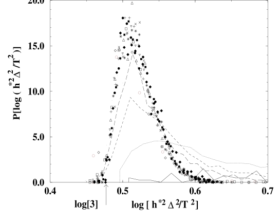
Figure 3: Histogram of $\log{((h^{*})^{2}\Delta^{2}/T^{2})}$, for different values of the Néel state magnetization $\Delta$. The lines correspond to $\Delta=1,2,3,4$ and the symbols to values of $\Delta$ between $5$ and $19$. The temperature is $T=0.4$. $2000$ clusters contained in the 20$\times$20 square were generated for each value of $\Delta$.

In the regime $\Delta\gg\sigma_{\beta}$, Eq. (7) becomes $(h^{*}/T)^{2}=3/\Delta^{2}$: the histograms in Fig. 3 would be a $\delta$ function located on the value $\log{3}$. Even if the histograms in Fig. 3 have a finite width, we see that the scaling $(h^{*}/T)^{2}\sim 1/\Delta^{2}$ still holds, at least for not too small values of $\Delta$. This suggests that $\sigma_{\beta}$ is not $\Delta$-independent but is rather distributed, and scales on average like $\Delta$. We attribute this behavior to the existence of low energy droplet excitations. Since these excitations correspond to large magnetic domains, the magnetization induced by reversing these domains should be coupled to the total Néel state magnetization $\Delta$.

3 Thermoremanent magnetization experiment

In this section, we recall how the function $X(C)$ characterizing the FDT violation can be obtained from the magnetization relaxation in the thermoremanent magnetization experiment. We first assume linear response. In the presence of a time-dependent magnetic field $h(t)$, the linear contribution to the magnetization is

$$m[h](t)=\int_{-\infty}^{t}R(t,t^{\prime})h(t^{\prime})dt^{\prime},$$ (10)

with $R$ the kernel response. We take here as a working hypothesis that

$$R(t,t^{\prime})=\beta X(C(t,t^{\prime}))\theta(t-t^{\prime})\frac{\partial C(t,t^{\prime})}{\partial t^{\prime}},$$ (11)

a form of the response kernel suggested by the mean field model studies [5, 7, 8]. The auto-correlation $C$ is

$$C(t_{w}+\tau,t_{w})=\overline{\langle\frac{1}{N}\sum_{i,j}\sigma_{i}(t_{w})\sigma_{j}(t_{w}+\tau)\rangle}.$$ (12)

In most of the spin-glass models (for instance: Sherrington-Kirkpatrick model, Edwards-Anderson model), the correlation length is vanishing, the reponse is purely local in space, and the terms $i\neq j$ vanish in (12). In the presence of a finite correlation length, the thermoremanent magnetization is conjugate to the spatially non local autocorrelation (12). From this point of view, (10),(11),(12) can be safely taken as a extension of $X(C)$ to our problem, in the sense that (i) lienar FDT reads $X(C)=1$ (ii) we recover the usual definition of $X(C)$ in the limit of a zero correlation length.

Barrat [16] used recently an interesting different method to handle spatially non local responses and non linearities: he measured the staggered magnetic response to a random field with a zero mean. In this way, the magnetic response to the random field is linear as a function of the width of the random field distribution, and conjugate to the local autocorrelations. We underline that Barrat does not consider the same conjugate quantities as ours, and the functions $X(C)$ are thus different. In particular, we cannot handle symmetry breaking within our framework. However, in the case of the present problem of magnetic systems on percolation clusters, the non linearities are quite weak and, as we will see, we can characterize their effects on dynamics, which could not be possible in the framework of Barrat calculations.

In the thermoremanent magnetization experiment, $h(t)$ is a step function $h(t)=h\theta(t_{w}-t)$, so that the thermoremanent magnetization reads

$$m(t_{w}+\tau,t_{w})=\beta h\int_{0}^{C(t_{w}+\tau,t_{w})}X(q)dq,$$

where we have assumed $C(t_{w}+\tau,0)=0$ [we have indeed checked that this quantity was vanishing in our simulations]. The function $X(C)$ is then obtained by differentiating the magnetic response

$$\chi(t_{w}+\tau,t_{w})=\frac{T}{h}m(t_{w}+\tau,t_{w})$$

with respect to the autocorrelation: $X(C)=d\chi/dC$. If the waiting time is large enough so that equilibrium has been reached, the magnetic response $\chi(\tau)$ is $t_{w}$-independent, $X(C)$ is unity, and we recover the linear FDT:

$$\chi(\tau)=\frac{T}{h}m(\tau)=C_{eq}(\tau).$$ (13)

Quite a lot of efforts have been devoted recently to characterize how the FDT is violated in an out-of-equilibrium situation. Analytical solutions were obtained in the framework of mean-field models [5, 7, 8]. The fluctuation-dissipation ratio was also obtained in numerical simulations in various models. For instance, in the case of spin glasses, Franz and Rieger [17] have analyzed the Edwards-Anderson model in three dimensions; more recently, Marinari et al. [18] have studied the FDT violation in three and four dimensional gaussian Ising spin glasses, and shown that the fluctuation-dissipation ration $X(C)$ is, in these models, equal to the static Parisi function $x(C)$. A model of fragile glass was also studied recently [19].

As explained in section 2, the magnetic response of percolating dilute antiferromagnets is not linear for magnetic fields of the order of $T/\sqrt{N}$. In the absence of linear response, the equilibrium magnetization can be expanded in powers of the magnetic field $h$, the coefficients of this expansion being the cumulants of the magnetization distribution (see Eq. (3)). Following the work of Gallavotti and Cohen [20], Kurchan [21] recently proposed an extension of the FDT to incoporate the effects of non linear response. However, we cannot use here this generalization in our Monte Carlo simulations since this would involve the calculation of the time-dependent magnetization distribution, included the tail where the magnetization is opposite to the magnetic field. For our purpose, we take here as a working phenomenological hypothesis that the thermoremanent magnetization is given by (10), with the magnetic-field dependent response kernel

$$R_{h}(t,t^{\prime})=\beta X_{h}(C(t,t^{\prime}))\theta(t-t^{\prime})\frac{\partial C(t,t^{\prime})}{\partial t^{\prime}}.$$

In the presence of non linearities and out-of-equilibrium dynamics, $X_{h}(C)$ contains contributions both from the non linearities and the aging dynamics. However, in the limit of large waiting times, the system has equilibrated and thus only the non linearities contribute to $X_{h}(C)$. In the opposite limit of small waiting times, the non linearities do not contribute to $X(C)$, and, in this limit, a contact can be made with FDT violations in other systems, especially euclidian coarsening dynamics [16].

4 Numerical results for $X(C)$

We now present our numerical calculations of $X(C)$. Our simulations were carried out on two clusters: a cluster $A$ with $N=836$ sites, $\Delta=36$, and a smaller cluster $B$ with $N=294$ sites and $\Delta=16$. These two clusters are shown in Fig. 4.

Figure 4: The two clusters that we studied. The cluster A contains $N=836$ sites, and $\Delta=36$. The cluster B contains $N=294$ sites, and $\Delta=16$.

We first present in section 4.1 the equilibrium dynamics: the waiting time is long enough for the system to have equilibrated in the external magnetic field, and, on the basis of the arguments presented in section 2, we expect sensible non linear effects. In fact, the relaxation time is finite even in the thermodynamic limit (interrupted aging). As the size of the system increases, the relaxation time will first increase, due to zero energy barriers scaling like $J\ln{N}$ [9], and saturate when the linear size $N^{1/\overline{d}}$ becomes larger than the correlation length given by [12]

$$\xi_{T}\sim\exp{\left(\frac{2J\nu_{P}}{T}\right)},$$

with $\nu_{P}$ the percolation critical exponent. The limit of small waiting times is next presented in section 4.2. In this situation, the magnetic response is linear. The combined effects of non linearities and out-of-equilibrium response arising for intermediate waiting times are next presented in section 4.3. Finally, the dependence on $\tau$ of the autocorrelation and the magnetic response are presented in section 4.4.

4.1 Large waiting times: equilibrium dynamics and non linear response

We first examine the regime of a large waiting time $t_{w}$, large enough for the magnetic response to be independent on $t_{w}$. In practice, we systematically checked that the magnetic response was unchanged when the waiting time was increased by a factor of $10$. The magnetic response $\chi_{h}$ is plotted as a function of the autocorrelation $C$ in Fig. 5 for the clusters A and B.

Figure 5: Variation of the magnetic response $\chi_{h}(C)$ versus the autocorrelation $C$ in equilibrium relaxation. The temperature is $T=0.8$, and the waiting time is $t_{w}=10^{5}$. The magnetic fields are $h=0.1$ (squares), $h=0.2$ (circles) and $h=0.3$ (crosses). The curves have been fitted along the procedure described in the text.

We clearly observe on Fig. 5 important non linear effects since the magnetic response $\chi_{h}$ depends explicitly on the magnetic field $h$, even at the relatively high temperature $T=0.8$. In the short time limit, we observe a behavior of the type $\chi_{h}(C)=C-C^{(0)}_{h}$, whereas in the long time limit, $\chi_{h}(C)=X^{(0)}_{h}C$. In order to interpolate between these two behaviors, we have fitted our numerical results to the form

$$X_{h}(C)=\frac{d\chi_{h}(C)}{dC}=(1-X^{(0)}_{h})f_{C^{*}_{h},\lambda_{h}}(C)+X^{(0)}_{h},$$ (14)

with

$$f_{C^{*}_{h},\lambda_{h}}(C)=\left(1+\exp{\left(-\frac{C-C^{*}_{h}}{\lambda_{h}}\right)}\right)^{-1},$$

where $\lambda_{h}$ controls the width of the cross-over between the short and the long time regimes, and $C^{*}_{h}=C^{(0)}_{h}/(1-X^{(0)}_{h})$. The fits obtained in this way are shown in Fig. 5, and, once the three parameters have been adjusted, a very good agreement with the simulation data is obtained. The variations of $X_{h}(C)$ deduced from the fits are shown in Fig. 6 for the same simulations as in Fig. 5.

Figure 6: Variation of $X_{h}(C)$ versus $C$ in equilibrium relaxation. The temperature is $T=0.8$. The variations of $X_{h}(C)$ are deduced from the simulations presented in Fig. 5.

We observe in Fig. 6 that $X_{h}(C)$ cross-overs from unity at short times to a finite value $X^{(0)}_{h}$ in the long time relaxation. If the response to the external magnetic field was linear, one would expect that $X(C)=1$. Even though we could not address this question here, we expect a non linear FDT of the type [21] to hold in the long waiting time limit.

4.2 Small waiting times: out-of-equilibrium dynamics and linear response

In the short waiting time limit, the thermoremanent magnetization is linear as a function of the magnetic field. We have shown in Fig. 7 the variations of the magnetic response $\chi$ versus the autocorrelation $C$ for the two values of the magnetic field $h=0.2,0.3$, and $t_{w}=10^{2},10^{3}$. Linear response is clearly observed. The variations of $X(C)$ are shown in the insert of Fig. 7.

Figure 7: Variations of the magnetic response $\chi(C)$ versus the autocorrelation $C$ in the short waiting time limit ($t_{w}=10^{2},10^{3}$), and $h=0.2,0.3$. The corresponding variations of $X(C)$ are shown in the insert.

Interestingly, the variations of $X(C)$ in this situation where out-of-equilibrium effects are dominant are qualitatively the same as the ones in section 4.1: $X$ cross-overs from unity at short times to a finite value in the long time limit. We have no understanding of the reason why the variations of $X(C)$ are qualitatively the same in the small and large waiting time limits, where deviations from linear FDT originate respectively from the out-of-equilibrium dynamics and non linear response.

The fact that $X(C)$ is finite in the aging regime is a quite noticeable difference with euclidian coarsening [16], where $X$ is vanishing in the aging regime (the linear response kernel $R$ in (10) is zero in this regime). The long term memory of coarsening dynamics on percolating structures is thus stronger than for euclidian dynamics, which is maybe not surprising on the general grounds recalled in the introduction: a “droplet” of size $N$ has a zero temperature energy barrier scaling like $\ln{N}$ [9, 10, 11], and a finite energy of the order of $2{\cal C}J$, ${\cal C}$ being the order of ramification [14].

4.3 Intermediate waiting times: out-of-equilibrium dynamics and non linear response

In order to examine the conjugate effects of nonlinearities in the magnetization response and out-of-equilibrium dynamics, we carried out the thermoremanent magnetization simulation with the cluster B at the temperature $T=0.55$, and for a waiting time $t_{w}=10^{6}$. The results are shown in Fig. 8, with $\tau$ up to $10^{7}$.

Figure 8: Variations of the magnetic response $\chi_{h}(C)$ versus the autocorrelation $C$ for the cluster B, $T=0.55$, $t_{w}=10^{6}$, $h=0.1$ (circles), $h=0.2$ (squares) , $0.3$ (crosses). The insert shows the corresponding variations of $X(C)$.

We have checked that equilibrium was not reached by carrying a simulation with a waiting time $t_{w}=10^{7}$. On the other hand, the magnetic response $\chi_{h}$ depends explicitly on the magnetic field $h$, as is visible in Fig. 8. We observe that $X_{h}(C)$ can still be fitted by the form (14), even though we could not reach very small values of the correlation and magnetic responses, even for $\tau=10^{7}$.

4.4 $\tau$-dependence of $\chi(t_{w}+\tau,t_{w})$ and $C(t_{w}+\tau,t_{w})$

In spin-glass models, the short time regime $\chi(t_{w}+\tau,t_{w})=C(t_{w}+\tau,t_{w})-C^{(0)}(t_{w})$ is valid up to a time $\tau^{*}$ of the order of the waiting time $t_{w}$ [17]. As shown in Fig. 9, we indeed observe such a dependence of $\tau^{*}$ in the out-of equilibrium situation: $\tau^{*}$ is of the order of $10^{2}$ for $t_{w}=10^{2}$, and of the order of $10^{3}$ for $t_{w}=10^{3}$. However, for larger waiting times, non linearities significantly reduce $\tau^{*}$ ($\tau^{*}\simeq 10^{3}$ for $t_{w}=10^{5}$ in Fig. 9 ).

Figure 9: Variations of $\chi(t_{w}+\tau,t_{w})+C^{(0)}(t_{w})$ (diamonds: $h=0.2$, crosses: $h=0.3$) and $C(t_{w}+\tau,t_{w})$ (solid lines) versus $\tau$. The waiting times are $t_{w}=10^{2},10^{3},10^{5}$. The temperature is $T=0.8$.

We observe in Fig. 10 in the case $t_{w}=10^{5}$, $T=0.8$ (equilibrium situation) that $\tau^{*}$ is also a function of the magnetic field $h$ (the value of $\tau^{*}$ for $h=0.1$ is one order of magnitude larger than for $h=0.2$). This effect is also visible in the out-of-equilibrium simulation shown in Fig. 10 ($T=0.55$). However, from our simulations, we cannot make a precise statement on the variations of $\tau^{*}$ as a function of $h$ for large waiting times.

Figure 10: Variations of $\chi(t_{w}+\tau,t_{w})+C^{(0)}(t_{w})$ (squares: $h=0.1$, diamonds: $h=0.2$, crosses: $h=0.3$) and $C(t_{w}+\tau,t_{w})$ (solid lines) versus $\tau$. The waiting times are $t_{w}=10^{5}$ ($T=0.8$), and $t_{w}=10^{6}$ ($T=0.55$).

5 Conclusions

We have thus carried out Monte Carlo simulations of the violation of the linear FDT in dilute percolating antiferromagnets. We have shown that these systems exhibit non linear response for magnetic fields of the order of $T/\sqrt{N}$. In the small waiting time regime, the thermoremanent magnetization is linear in the magnetic field, but depends explicitly on the waiting time. On the other hand, for sufficiently large waiting times, the system has equilibrated (interrupted aging), and the magnetic response is non linear. Interestingly, in both situations, as well as in the intermediate situation where both out-of-equilibrium and non linear effects come into account, the function $X(C)$ characterizing the deviations from linear FDT has qualitatively the same shape: it is unity at short times and cross-overs to a constant finite value for long times, the cross-over occurring at $\tau^{*}$. In the small waiting time limit, $\tau^{*}$ is of the order of the waiting time $t_{w}$. For larger waiting times, non linearities strongly reduce $\tau^{*}$ as the magnetic field is increased. By comparison with domain growth processes in non diluted lattices, the aging part of the dynamics shows stronger long-term memory, due to the existence of large scale low-energy ‘droplet’ excitations.

Acknowledgments R.M. thanks A. Barrat, L.F. Cugliandolo, J. Kurchan, S. Franz and P.C.W. Holdsworth for stimulating discussions. Part of the calculations presented here were carried out on the CRAY T3E computer of the Centre de Calcul Vectoriel Grenoblois of the Commissariat à l’Energie Atomique.

References

- [1] L. Lundgren, P. Svedlindh, P. Norblad and O. Beckman, Phys. Rev. Lett. 51 (1983) 911; P. Norblad, L. Lundgren, P. Svedlindh and L. Sandlund, Phys. Rev; B 33 (1988) 645; L. Lundgren, J. Phys. Colloq France 49 (1988) C8-1001 and references therein.
- [2] M. Alba, M. Ocio and J. Hamman, Europhys. Lett. 2 (1986) 45; J. Phys. Lett. France 46 (1985) L-1101; M. Alba, J. Hamman, M. Ocio and P. Refregier, J. Appl. Phys. 61 (1987) 3683; E. Vincent, J. Hamman and M. Ocio, Recent Progress in Random Magnets, D.H. Ryan Ed. (World Scientific, Singapore, 1992).
- [3] D.S. Fisher and D.A. Huse, Phys. Rev. Lett. 56 (1986) 1601; Phys. Rev. B 38 (1988) 373.
- [4] G.J. Koper and H.J. Hilhorst, Physica A 155 (1989) 431.
- [5] L.J. Cugliandolo and J. Kurchan, Phys. Rev. Lett. 71 (1993) 173; J. Phys. A 27 (1994) 5749.
- [6] J.P. Bouchaud, J. Phys. I France 2 (1992) 1705; J.P. Bouchaud, E. Vincent and J. Hamman, J. Phys. I France 4 (1994) 139; J.P. Bouchaud and D.S. Dean, J. Phys. I France 5 (1995) 265.
- [7] A. Baldassari, L.F. Cugliandolo, J. Kurchan and G. Parisi, J. Phys. A 28, 1831 (1995).
- [8] L.F. Cugliandolo and D.S. Dean, J. Phys. A 28, 4213 (1995).
- [9] R. Rammal and A. Benoît, J. Phys. Lett. 46 (1985) L 667; Phys. Rev. Lett. 55 (1985) 649.
- [10] R. Rammal, J. Phys. France 46 (1985) 1837.
- [11] C.L. Henley, Phys. Rev. Lett. 54 (1985) 2030.
- [12] A. Coniglio, Phys. Rev. Lett. 46 (1981) 250.
- [13] R.H. Swendsen and J.S. Wang, Phys. Rev. Lett. 57 (1986) 2606; Phys. Rev. Lett. 58 (1987) 86. See also R.H. Swendsen, J.S. Wang and A.M. Ferrenberg in The Monte Carlo Method in condensed Matter Physics, Topics in Applied Physics Vol. 71, K. Binder Ed. (Springer-Verlag, Berlin-Heidelberg-New York, 1992).
- [14] S. Kirkpatrick, in Les Houches Summer School on Ill Condensed Matter Physics, R. Ballian, R. Maynard and G. Toulouse Eds. (North Holland, Amsterdam, 1979).
- [15] R. Mélin, J. Phys. I, France 6 (1996) 793.
- [16] A. Barrat, Report No cond-mat/9710069.
- [17] S. Franz and H. Rieger, J. Stat. Phys. 79, 749 (1995).
- [18] E. Marinari, G. Parisi, F. Ricci-Tersenghi and J.J. Ruiz-Lorenzo, Report No cond-mat/9710120.
- [19] G. Parisi, Phys. Rev. Lett. 79 (1997) 3660.
- [20] G. Gallavotti and E.G.D. Cohen, Phys. Rev. Lett. 74, 2694 (1995); J. Stat. Phys. 80, 931 (1995); G. Gallavotti, Phys. Rev. Lett. 77, 4334 (1996).
- [21] J. Kurchan, Report No cond-mat/9709304.