Dynamical simulation of current fluctuations in a dissipative two-state system
Abstract
Current fluctuations in a dissipative two-state system have been studied using a novel quantum dynamics simulation method. After a transformation of the path integrals, the tunneling dynamics is computed by deterministic integration over the real-time paths under the influence of colored noise. The nature of the transition from coherent to incoherent dynamics at low temperatures is re-examined.
pacs:
PACS numbers: 02.70.Lq, 05.30.-d, 05.40.+jA two-state system coupled to a dissipative environment is the archetypical model for tunneling phenomena in condensed phase. It has found widespread applications in solid-state physics [1, 2, 3], most recently in interlayer charge transport in high- superconductors [4] and quantum computing[5], as well as in biophysics [6] for the modeling of electron transport in biochemical reactions. One of the most intriguing features of this model is a dynamical phase transition between coherent tunneling and incoherent relaxation. This was first predicted by Chakravarty and Leggett [7, 8] and later confirmed by experiments on interstitial tunneling in niobium[9].
Although the existence of the coherent-incoherent transition is widely accepted, its precise nature and location has been called into question by some recent calculations [10, 11, 12, 13]. Coherence is a phenomenon of dynamics, yet an exact treatment of tunneling in the time domain has so far been out of reach. The original prediction of the transition [8] was based on a dynamical but approximate theory, whereas the more recent theories, suggesting the transition would occur at a much weaker damping than predicted earlier, were based on statistical mechanical calculations [10, 11].
In this Letter, we describe a new exact numerical method for calculating the real-time dynamics of dissipative quantum systems and use it to investigate the transition from coherent to incoherent dynamics in a two-state system at low temperatures. Previously, the only exact numerical approach to tunneling dynamics has been the dynamical quantum Monte Carlo (QMC) method [12, 14]. But all real-time QMC simulations fail at longer times because the signal-to-noise ratio of the results vanishes exponentially due to the highly oscillatory integrand. This problem is commonly referred to as the dynamical sign problem. In the case of large bandwidth of the dissipative environment, QMC simulations further suffer from a slowing-down problem caused by the increasingly long-lived correlations in the sampling process. The new method eliminates both problems through a generalized Hubbard-Stratonovich transformation and allows us to perform the functional integration over paths of the tunneling system by a deterministic method, while statistically sampling fluctuations from an ensemble of Gaussian noise trajectories.
Dissipative two-state systems are often described by the spin-boson model,
| (2) | |||||
where is the position operator of the tunneling system with intrinsic tunneling frequency , and are Pauli spin matrices, and . The effect of the harmonic environment is fully characterized by a spectral density , for which the Ohmic form is experimentally the most relevant and theoretically the most interesting. The Ohmic spectral density introduces a single dimensionless damping constant . This model must be regularized by an upper cutoff of the spectral density. The scaling limit is characteristic of tunneling in solids and as shown by scaling arguments[15], the Ohmic spin-boson model has nontrivial dynamics only for , and the renormalized tunneling frequency
| (3) |
is the only frequency scale of the dynamics at zero temperature other than . The transition from coherent to incoherent dynamics occurs at a critical damping at which the factor of the tunneling oscillations vanishes. Tunneling oscillations can be observed as a damped oscillatory component of the position correlation function that is present in addition to an incoherent relaxation background[16]. The asymptotic long-time behavior is always dominated by an algebraic incoherent decay, [17].
A coherence criterion equivalent to finite is a finite dephasing time of the quantum beats that manifest themselves as tunneling oscillations. A measure of this dephasing time is given by the lifetime of delocalized states of the tunneling system [18] (see also[13, 19]) , which are eigenstates of the tunneling current . The correlation time of the current correlation function
| (4) |
equals the lifetime of these superposition states. A finite correlation time of the current correlation function thus implies coherent oscillations in the position correlation function. This relationship allows us to identify coherence even for very strongly damped cases in which oscillations may be masked by the incoherent background. For a two-state system, the relation provides another direct connection to previous studies on the position correlation function.
To compute the exact dynamics of , we employ a hybrid stochastic/deterministic numerical method which we shall label chromostochastic quantum dynamics (CSQD). This method, which is generally applicable to quantum systems with linear dissipation, is based on the path integral formulation of dissipative quantum dynamics[8, 20]. The time evolution of the reduced density matrix for the system coordinate can formally be represented by a double functional integral[21]
| (5) |
is the action of the undamped quantum system, and its interactions with the environment are incorporated into a complex-valued influence functional with
| (7) | |||||
| (9) | |||||
is the real part of the autocorrelation function of the collective bath mode , averaged over an ensemble of free oscillators, is the mass of the tunneling particle, and is the classical friction kernel associated with the spectral density . This influence functional describes a ‘factorized’ initial preparation, i.e. with the particle constrained to one side for times with the environment fully relaxed. To simulate equilibrium correlation functions, it is necessary to push the preparation back to a sufficiently large negative time [20] and insert measurement operators at times and .
A direct quantum Monte Carlo evaluation of a time-discretized version of type (5) can be prohibitively expensive due to the dynamical sign and slowing-down problems. An alternative approach for single-particle problems or dissipative systems near the Markovian limit is the explicit iteration of a short-time propagator. This reduces the path integral to a manageable series of matrix multiplications[22]. Another algorithm was recently presented by Cao, Unger and Voth[23] for an environment with a few oscillators. By directly sampling the oscillator paths and propagating the system coordinate for each sample, they eliminate memory effects.
In this Letter, we tackle the problem of memory effects in the important case of a continuum of environmental modes, such as in the case of Ohmic friction, where sampling over individual oscillator trajectories is not feasible. The major obstacle in trying to decompose the path integral (5) into short-time propagators lies in the interaction kernel because its range diverges as the temperature approaches zero. In comparison, the friction kernel poses no problem because it vanishes at time larger than , the shortest timescale in our problem.
The problem with the long-range interactions introduced by can nonetheless be solved, albeit at the cost of introducing an additional path variable. The exponential of the non-local action can be decomposed into a superposition of time-local phase factors,
| (10) | |||
| (11) |
The distribution is real and Gaussian, with , and normalizable through the condition . Formally, this decomposition is a Hubbard-Stratonovich transformation in a function space over the interval . Equation (10) is equivalent to the construction of an influence functional for a classical colored noise source[21], and as such, we will interpret the function as a noise trajectory.
In the CSQD algorithm, the propagation of the system coordinates and is carried out deterministically for each realization of the noise trajectory, while the noise trajectories are sampled from the distribution . Instead of generating weights from a Metropolis-type random walk, statistical weights are assigned to noise trajectories a priori by numerically filtering white noise.
In general, there are two ways to treat the remaining term . If acts on a finite-dimensional Hilbert space, contains discrete jumps between the eigenvalues of . The ‘state vector’ that is propagated must then remember these ‘virtual transitions’ during a finite number of preceding time slices. But since the friction kernel decays rapidly over the memory time , the number of transitions needed ‘in memory’ is small for large cutoff. On the other hand, if describes a continuous degree of freedom, the kinetic term in requires the relevant paths to be smooth. Then the limit can be applied to (9), making a time-local functional.
For the two-state system, we achieve excellent accuracy with a maximum of two tunneling events ‘in memory’. The error resulting from this truncation can be made arbitrarily small by increasing , i.e., moving further into the scaling regime[24]. The length of our time steps is a fixed fraction of the inverse bandwidth , which is short enough to make the particular choice of approximate short-time propagator a minor issue.
Empirically, we find that the statistical variance of CSQD grows no faster than logarithmically with . This remarkable performance compared to the exponential divergence observed in conventional QMC methods results from the fact that deterministic integration is not affected by the oscillatory nature of the integrand. Consecutive samples in the CSQD simulation are by design statistically independent. This completely eliminates any slowing-down problem. We have tested the validity and accuracy of our method, comparing to known analytic results for the real-time fluctuations and the relaxation behavior of the tunneling coordinate at damping and . We find excellent agreement between our numerical results and previous analytic calculations.
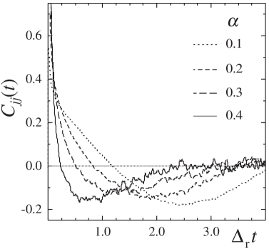
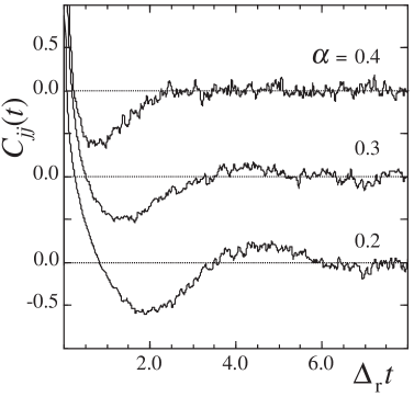
Fig. 1 shows CSQD results for at zero temperature and for . Except for the initial drop at times , all four curves represent functions of the scaling argument only. To obtain a formal estimate for , we define it to be the first zero of [25]. Positive current-current correlations do persist up to times of order , i.e., the scaled dephasing time is nonzero and finite (at least) up to , although it declines significantly with increasing . Quantum coherence becomes increasingly short-lived, however, making it impossible to resolve oscillations from a background of monotonous signal decay for (Fig. 2).
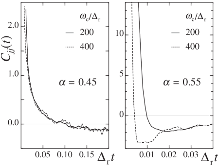
An expanded view of the initial decay of in the vicinity of the critical value is provided in Fig. 3. In this region, the correlation time decreases rapidly with increasing (note the different scales on the time axes). Comparing results for different cutoff frequencies , we observe markedly different scaling behavior for above or below . For , is scaled by , leaving finite; whereas for , scales as , i.e. vanishes in the scaling limit.
Critical behavior at is also predicted by perturbation theory in the bare tunneling frequency . In the scaling limit, the short-time behavior of the current correlation function is given by
| (12) |
For , this expression (valid for ) as well as the exact perturbative result (valid for ) is
positive. It follows that , which can only be satisfied if scales with rather than . For , (12) is negative, and we conclude that turns negative at a time of the order of .
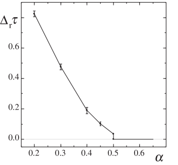
Taken together, these results lead to a clear picture of how the scaled dephasing time depends on the damping strength, shown in Fig. 4. We see a gradual decline of to very small but finite values, followed by a discontinuous drop at . The finite value at emerges both from our simulations and from applying to analytic results for the position correlation function at [16, 26].
Our conclusion coincides exactly with the value originally found by Chakravarty and Leggett[7] for the dynamics of a two-state system with a factorized initial preparation. In contrast, Lesage, Saleur, and Skorik[10] as well as Costi and Kiefer[11] recently found a lower value
for the critical damping. In both their works, the criterion of coherence was not the observation of tunneling oscillations themselves, but the presence of inelastic peaks in the spectral function of the position fluctuations. For strongly damped oscillations in the symmetric function , however, the inelastic peaks at positive and negative frequencies become wide enough to merge into a single peak centered at . The absence of a peak at finite frequency therefore does not necessarily indicate the absence of coherence. In order to determine the true critical coupling, a more elaborate analysis needs to be performed on the spectra of [10, 11].
In conclusion, we have introduced a new numerical algorithm for the dynamics of dissipative quantum systems, which solves the dynamical sign problem and eliminates slowing-down problems. Its validity, efficiency and accuracy have been demonstrated for the spin-boson model with Ohmic dissipation. We have determined the lifetime of coherent superposition states at zero temperature and different strengths of the damping from the current correlation function. This timescale decreases with increasing damping strength , but remains finite (indicating quantum coherence) for all below the critical value . Analytic results, where available, are reproduced with good agreement. Details of the CSQD method and its applications to more complex problems such as the noise spectrum of fractional quantum Hall systems will be reported elsewhere.
This research has been supported by the National Science Foundation under grant CHE-9528121. CHM is a NSF Young Investigator (CHE-9257094), a Camille and Henry Dreyfus Foundation Camille Teacher-Scholar and a Alfred P. Sloan Foundation Fellow. Computational resources have been provided by the IBM Corporation under the SUR Program at USC.
REFERENCES
- [1] H. Grabert and H. Wipf, in Advances in Solid State Physics, Vol. 30, 1 (Vieweg, Braunschweig, 1990).
- [2] B. Golding, N.M. Zimmerman, and S.N. Coppersmith, Phys. Rev. Lett. 68, 998 (1992).
- [3] S. Chakravarty and S. Kivelson, Phys. Rev. Lett. 50, 1811 (1983).
- [4] S. Chakravarty and P.W. Anderson, Phys. Rev. Lett. 72, 3859 (1994).
- [5] A. Garg, Phys. Rev. Lett. 77, 964 (1996).
- [6] R.A. Marcus and N. Sutin, Biochim. Biophys. Acta. 811, 265 (1985).
- [7] S. Chakravarty and A.J. Leggett, Phys. Rev. Lett. 52, 5 (1984).
- [8] A.J. Leggett, S. Chakravarty, A.T. Dorsey, M.P.A. Fisher, A. Garg and W. Zwerger, Rev. Mod. Phys. 59, 1 (1987), ibid., 67,
725 (1995).