[

Universality of Shot-Noise in Multiterminal Diffusive Conductors

Abstract

We prove the universality of shot-noise in multiterminal diffusive conductors of arbitrary shape and dimension for purely elastic scattering as well as for hot electrons. Using a Boltzmann-Langevin approach we reduce the calculation of shot-noise correlators to the solution of a diffusion equation. We show that shot-noise in multiterminal conductors is a non-local quantity and that exchange effects can occur without quantum phase coherence even at zero electron temperature. Concrete numbers for shot-noise are given that can be tested experimentally.

]

Shot-noise [4] induced by current or voltage fluctuations in electron transport is a striking manifestation of charge quantization. It serves as a sensitive tool to study correlations in conductors: while shot-noise assumes a maximum value (with Poissonian distribution) in the absence of correlations, it becomes suppressed when correlations set in as e.g. imposed by the Pauli principle [5, 6, 7, 8] or by electron-electron interactions [9, 10].

In diffusive mesoscopic two-terminal conductors where the inelastic scattering lengths exceed the system size the shot-noise suppression factor for “cold” electrons (i.e. for vanishing electron temperature) was predicted [11, 12, 13, 14, 15] to be $1/3$. The suppression of shot-noise in diffusive conductors is now experimentally confirmed [16, 17, 18, 19]. While some derivations [11, 13, 14, 15] are based on a scattering matrix approach and thus a priori include quantum phase coherence, no such effects are included in the semiclassical Boltzmann-Langevin equation approach, which nevertheless leads to the same result [12]. However, while in the quantum approach for a two-terminal conductor the factor $1/3$ was even shown to be universal [14], the semiclassical derivations given so far [12, 4] are restricted to quasi–onedimensional conductors. For this reason the factor $1/3$ was subsequently challenged by Landauer as a numerical coincidence [20], which then raises the intriguing question whether phase coherence is relevant or not for shot-noise in diffusive conductors.

Motivated by this situation we obtain new results here that will shed new light on this question. In particular, we will demonstrate that the shot-noise suppression factor of $1/3$ is universal also in the semiclassical Boltzmann-Langevin approach, in the sense that it holds for a multiterminal diffusive conductor of arbitrary shape and disorder distribution. We first prove this for cold electrons and then for the case of hot electrons where the suppression factor is $\sqrt{3}/4$. Thereby we extend previous semiclassical investigations[9, 10] for two-terminal conductors to an arbitrary multiterminal geometry. This allows us then to compare our semiclassical approach with the scattering matrix approach for multiterminal conductors [8, 21, 22], in particular with some explicit results recently obtained for diffusive conductors [15]. While the universality of shot-noise proven here still does not rule out a numerical coincidence [20] completely, it certainly makes it less likely and thereby gives further support to the suggestion [23] that phase coherence is not essential for the suppression of shot-noise in diffusive conductors.

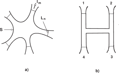
FIG. 1.: a) Multiterminal diffusive conductor of arbitrary 2D or 3D shape and with arbitrary impurity distribution. There are $N$ leads with metallic contacts of area $L_{n}$, and $I_{m}$ is the m-th outgoing current. $S$ denotes the remaining surface of the conductor where no current can pass through. b) H-shaped conductor with four leads of equal conductances, $G/4$, connected by a wire in the middle of conductance $G_{0}$.

Another remarkable property of shot-noise in mesoscopic conductors is the exchange effect introduced by Büttiker [21]. Although this effect is generally believed to be phase-sensitive, we will show that this need not be so. Indeed, for the particular case of an H-shaped conductor (see Fig. 1b) we show that exchange effects can be of the same order as the shot-noise itself even in the framework of the semiclassical Boltzmann approach. These exchange effects are shown to come from a non-linear dependence on the local distribution function. Similarly we show that the same non-linearities are responsible for non-local effects such as the suppression of shot-noise by open leads even at zero electron temperature.

Finally, we will illustrate the general formalism introduced here by concrete numbers for various conductor shapes that are of direct experimental interest.

Diffusive conductors. We consider a multiterminal mesoscopic diffusive conductor of arbitrary 2D or 3D shape (see Fig. 1) which is connected to $N$ perfect metallic contacts of area $L_{n}$, $1\leq n\leq N$, where the voltages $V_{n}$ or outgoing currents $I_{n}$ are measured. Our goal is to calculate the multiterminal spectral density $S_{nm}^{c}$ of current fluctuations $\delta I_{n}(t)$ at zero frequency $\omega=0$, defined by

$$S^{c}_{nm}=\int\limits_{-\infty}^{\infty}dt\langle\delta I_{n}(t)\delta I_{m}(0)\rangle.$$ (1)

We start from the (semiclassical) Boltzmann-Langevin equation for the distribution function [24, 25]. Using standard diffusion approximations and neglecting the accumulation of charge (we are interested in $\omega=0$ limit) we get the following equations [9] for the symmetric $f_{0}(\varepsilon,{\bf r})$ and antisymmetric ${\bf f}_{1}(\varepsilon,{\bf r})$ parts of the average distribution function $f(\varepsilon,{\bf r})=f_{0}(\varepsilon,{\bf r})+{\bf n}\!\cdot\!{\bf f}_{1}(\varepsilon,{\bf r})$,

$$\nabla[\sigma\nabla f_{0}]+I_{ee}[f]+I_{e-ph}[f]=0,\,\,{\bf f}_{1}=-v_{F}\tau_{im}\nabla f_{0},$$ (2)

and for the fluctuations $\delta{\bf j}({\bf r},t)$ and $\delta V({\bf r},t)$ of the current density and of the potential, resp.,

$$\delta{\bf j}+\sigma\nabla\delta V=\delta{\bf j}^{s},\,\,\,\nabla\cdot\delta{\bf j}=0,$$ (3)

and where the correlator of the Langevin fluctuation sources is given by

$$\langle\delta j^{s}_{\alpha}({\bf r},t)\delta j^{s}_{\beta}({\bf r}^{\prime},t^{\prime})\rangle = \delta_{\alpha\beta}\delta(t-t^{\prime})\delta({\bf r}-{\bf r}^{\prime})\sigma({\bf r})\Pi({\bf r}),$$ (4)

$$\Pi({\bf r}) = 2\int d\varepsilon f_{0}(\varepsilon,{\bf r})[1-f_{0}(\varepsilon,{\bf r})].$$ (5)

Here we introduced the local conductivity $\sigma({\bf r})=\gamma e^{2}\nu_{F}v_{F}^{2}\tau_{im}({\bf r})$ ($\gamma_{3D,2D}=1/3,1/2$), electron-electron $I_{ee}[f]$ and electron-phonon $I_{e-ph}[f]$ collision integrals, and used the fact that the electron number is conserved, $\int d\varepsilon I_{ee}[\delta f]=\int d\varepsilon I_{e-ph}[\delta f]=0$, where $\delta f$ is the fluctuation around the $f$. We also neglected momentum relaxation due to electron-phonon interaction; but note that we allow for inhomogeneous disorder, i.e. $\tau_{im}=\tau_{im}({\bf r})$.

Now we specify the boundary conditions to be imposed on Eqs. (2,3). First, we assume that for a given energy there is no current through the surface $S$. Second, since the contacts with area $L_{n}$ are perfect conductors the average potential $V$ and its fluctuations $\delta V$ are independent of position ${\bf r}$ on $L_{n}$. Third, the contacts are assumed to be in thermal equilibrium with outside reservoirs. The boundary conditions for (2) and (3), resp., then read explicitly

$$f_{0}(\varepsilon,{\bf r})\left|\right._{L_{n}}=f_{T}(\varepsilon-eV_{n}),\quad d{\bf s}\!\cdot\!\nabla f_{0}(\varepsilon,{\bf r})\left|\right._{S}=0,$$ (6)

$$d{\bf s}\!\cdot\!\delta{\bf j}({\bf r},t)\left|\right._{S}=0,\quad\delta V({\bf r},t)\left|\right._{L_{n}}=\delta V_{n}(t),$$ (7)

where $f_{T}(\varepsilon)$ is the equilibrium distribution function at temperature $T$, and $d{\bf s}$ is a vector area element perpendicular to the surface.

We derive now the exact solution of Eqs. (2,3) with boundary conditions (6,7) and use it to evaluate $S_{nm}^{c}$ for a multiterminal conductor of arbitrary shape and distribution of impurities. For this it is convenient to follow Ref.[26] and to introduce $N$ characteristic potentials $\phi_{n}({\bf r})$ which satisfy the diffusion equation with associated boundary conditions:

$$\nabla[\sigma\nabla\phi_{n}]=0,\quad d{\bf s}\!\cdot\!\nabla\phi_{n}\left|\right._{S}=0,\quad\phi_{n}\left|\right._{L_{m}}=\delta_{nm},$$ (8)

with $\phi_{n}\geq 0$ and the sum rule $\sum_{n=1}^{N}\phi_{n}=1$. The potential $V$ (and thus the current ${\bf j}=\sigma\nabla V$) can then be expressed in terms of $\phi_{n}$, $V=\sum_{n}\phi_{n}V_{n}$, and the conductance then follows as $G_{nm}=-\int_{L_{n}}d{\bf s}\!\!\ \cdot\!\ \sigma\nabla\phi_{m}$. Next we multiply the first part of (3) by $\nabla\phi_{n}$ and integrate it over the volume. Subsequent partial integration of the lhs  gives the solution of (3) in terms of $\phi_{n}$: $\delta\tilde{I}_{n}(t)\equiv\delta I_{n}(t)-\sum_{m}G_{nm}\delta V_{m}(t)=\int d{\bf r}\nabla\phi_{n}\!\cdot\!\delta{\bf j}^{s}$. Using the correlator (5) we obtain a generalized multiterminal spectral density $S_{nm}=\int_{-\infty}^{\infty}dt\langle\delta\tilde{I}_{n}(t)\delta\tilde{I}_{m}(0)\rangle$:

$$S_{nm}=\int d{\bf r}\sigma\Pi\nabla\phi_{n}\!\cdot\!\nabla\phi_{m},$$ (9)

with the properties: $S_{nm}=S_{mn}$ and $\sum_{n}S_{nm}=0$. Eq. (9) is valid for elastic and inelastic scatterings and for an arbitrary multiterminal diffusive conductor. The relation of $S_{nm}$ to the measured noise is now as follows. If, say, the voltages are fixed, then $\delta I_{n}(t)=\delta\tilde{I}_{n}(t)$, and the matrix $S_{nm}=S_{nm}^{c}$ is directly measured. On the other hand, when currents are fixed, $S_{nm}$ can be obtained from the measured voltage correlator $S^{v}_{nm}=\int_{-\infty}^{\infty}dt\langle\delta V_{n}(t)\delta V_{m}(0)\rangle$ by tracing it with conductance matrices: $S_{nm}=\sum_{n^{\prime}m^{\prime}}G_{nn^{\prime}}G_{mm^{\prime}}S_{n^{\prime}m^{\prime}}^{v}$. The physical interpretation of (9) becomes now transparent: $\Pi$ describes the broadening of the distribution function (effective temperature) that is induced by the voltage applied to the conductor and $\sigma\Pi$ can thus be thought of as a local noise source, while $\phi_{n}$ can be thought of as the probe of this local noise. In particular, this means that only $S_{nm}$ is of physical relevance but not the current or voltage correlators themselves. We note that (9) together with Eqs. (2,6,8) can serve as a starting point for numerical evaluations of $S_{nm}$. For purely elastic scattering as well as for hot electrons it is even possible to get closed analytical expressions for $S_{nm}$ as we will show next. The physical conditions for the different transport regimes are discussed in Ref. [9].

Elastic scattering: $I_{ee}=I_{e-ph}=0$. For simplicity we work now in the $T=0$ limit (the generalization to $T>0$ is straightforward [27]). First we note that $f_{0}$ satisfies the diffusion equation $\nabla[\sigma\nabla f_{0}]=0$ with boundary conditions (6). The solution in terms of $\phi_{n}$ then is, $f_{0}=\sum_{n}\phi_{n}\theta(\varepsilon-eV_{n})$. Substituting this $f_{0}$ into $\Pi$ in (5) we obtain

$$\Pi=e\sum\limits_{k,l}\phi_{k}\phi_{l}\left|V_{k}-V_{l}\right|,$$ (10)

which in combination with Eq. (9) gives the general expression for $S_{nm}$ in the case of elastic scattering.

Now we are in the position to generalize the proof of universality of the $1/3$-suppression of shot-noise [11, 12, 13, 14] to the case of an arbitrary multiterminal diffusive conductor. To be specific we choose $V_{n}=\delta_{n1}V_{1}$, i.e. only contact one has a non-vanishing voltage. Then, using $\sum_{n}\phi_{n}=1$, we get $\Pi=2eV\phi_{1}[1-\phi_{1}]$. Substituting this into (9) and integrating by parts we obtain, $S_{1n}=2eV\oint d{\bf s}\!\cdot\!\nabla\phi_{n}\sigma[\phi_{1}^{2}/2-\phi_{1}^{3}/3]=-{1\over 3}eI_{n}$. For $n=1$ we have $S_{11}={1\over 3}eI$, where $I\equiv-I_{1}>0$ is the incoming current. Thus, the factor ${1\over 3}$ is indeed universal in the sense that it does not depend on the shape of the conductor nor on its impurity distribution. This generalizes the known universality of a two–terminal conductor [14] to a multiterminal geometry.

Next we specialize to two experimentally important cases. First we consider a multiterminal conductor of a star geometry with $N$ long leads (but with otherwise arbitrary shape) that join each other at a small crossing region. The resistance of this region is assumed to be much smaller than the resistance of the leads. In the second case the contacts are connected through a wide region, where again the resistance of the conductor comes mainly from the regions near the contacts, while the resistance of the wide region is negligible. Both shapes are characterized by the requirement that $w/L\ll 1$, where $w$ and $L$ are the characteristic sizes of the contact and of the entire conductor, resp. In both cases the conductor can be divided into $N$ subsections associated with a particular contact so that the potential $V$ is approximately constant (for $w/L\ll 1$) on the dividing surfaces. $G_{nm}$ can then be expressed in terms of the conductances of these subsections (denoted by $G_{n}$),

$$G_{nm}=(\alpha_{m}-\delta_{nm})G_{n},\quad\alpha_{m}\equiv G_{m}/G,$$ (11)

where $G\equiv\sum_{n}G_{n}$. Applying now similar arguments as above in the proof of the 1/3-suppression we find[27] the explicit expressions

$$S_{nm} = {1\over 3}e\sum\limits_{k}\alpha_{n}\alpha_{k}(J_{k}+J_{n})(\delta_{nm}-\delta_{km}),$$ (12)

$$J_{n} = \sum\limits_{l}G_{l}|V_{n}-V_{l}|.$$ (13)

We note that this result is valid up to corrections of order $w/L$ in 3D and for a star geometry in 2D, and up to corrections of order $[\ln(L/w)]^{-1}$ for wide conductors in 2D[27].

We are now in the position to address the issue of non-locality of noise in multiterminal conductors. For this we consider for instance a star geometry and assume that the current enters the conductor through the $n$-th contact, i.e. $I_{n}=-I$, and leaves it through the $m$-th contact, i.e. $I_{m}=I$, while the other contacts are open, i.e. $I_{k}=0$ for $k\neq n,m$. From (11) we obtain for the conductance $G_{n}G_{m}/(G_{n}+G_{m})$ (two contacts are in series), and we see that it does not depend on the other leads, which simply reflects the local nature of diffusive transport. However, contrary to one’s first expectation, this locality does not carry over to the noise in general. Indeed, from (13) it follows that $S_{nm}=-{1\over 3}(\alpha_{n}+\alpha_{m})eI$. The additional suppression factor $0<\alpha_{n}+\alpha_{m}<1$ for $N>2$ reflects the non-locality of the current noise. For instance, for a cross with $N=4$ equivalent leads we have $\alpha_{m}=\alpha_{n}=1/4$, and thus $S_{nm}=-{1\over 6}eI$. An analogous reduction factor was obtained in Ref. [11] under a different point of view. Hence, one cannot disregard open contacts simply because no current is flowing through them; on the contrary, these open contacts which are still connected to the reservoir induce equilibration of the electron gas and thereby reduce its current noise. We emphasize that this non-locality is a purely classical effect in the sense that no quantum phase interference is involved (phase coherent effects are not contained in our Boltzmann approach); the origin of this non-locality can be traced back to the non-linear dependence of $\Pi$ on the distribution $f$ in (5).

Next we discuss exchange effects [21] in a four terminal conductor. According to Blanter and Büttiker [15] they can be probed by measuring $S_{13}$ in three ways: $V_{n}=V\delta_{n2}$ (A), $V_{n}=V\delta_{n4}$ (B), and $V_{n}=V\delta_{n2}+V\delta_{n4}$ (C). Then we take $\Delta S_{13}=S_{13}^{C}-S_{13}^{A}-S_{13}^{B}$ as a measure of the exchange effect. It comes now as some surprise that in our semiclassical Boltzmann approach $\Delta S_{13}$ turns out to be non-zero in general and can even be of the order of the shot-noise itself. Again, the reason for that is that $\Pi$ is non-linear in $f_{0}$ (see (5)). So, the value $\Pi^{C}-\Pi^{A}-\Pi^{B}$ which enters $\Delta S_{13}$ is not necessarily zero. Indeed, while exchange effects vanish for cross shaped conductors (in agreement with [15] up to corrections of order $w/L$ which are neglected in our approximation), it is not so for an H-shaped conductor (see Fig. 1b). Calculations similar to those leading to (13) give for this case[27]: $\Delta S_{13}={1\over{24}}eVG^{2}G_{0}/(G+4G_{0})^{2}$, where $G_{n}=G/4$ are the conductances (all being equal) of the outer four leads, while the conductance of the connecting wire in the middle is denoted by $G_{0}$. This exchange term $\Delta S_{13}$ vanishes for $G_{0}\to\infty$, because then the case of a simple cross is recovered, and also for $G_{0}\to 0$, because then the $1$-st and $3$-rd contacts are disconnected. $\Delta S_{13}$ takes on its maximum value for $G_{0}=G_{n}$ and becomes equal to ${1\over{60}}eI^{A}$, where $I^{A}$ is the current through the $2$-nd contact for case (A). Although $\Delta S_{13}$ is positive in this example this is not the case in general [27].

In principle, (13) and (11) allow us to calculate the noise for arbitrary voltages, but for illustrative purposes we consider again the simple case of a cross-shaped conductor with four equivalent leads, i.e. $\alpha_{n}=1/4$. Suppose the voltage is applied to only one contact, say $V_{1}=V$, $V_{n\neq 1}=0$, and $I=-I_{1}=3I_{n\neq 1}$. Then, from (13) we obtain: $S_{11}={1\over 3}eI$, $S_{12}=S_{13}=S_{14}=-{1\over 9}eI$, all being in agreement with the universal $1/3$-suppression proven above. Then, $S_{22}=S_{33}=S_{44}={2\over 9}eI$, and $S_{23}=S_{24}=S_{34}=-{1\over{18}}eI$ [28]. These numbers seem to be new and it would be interesting to test them experimentally.

Hot Electrons. In this case $I_{ee}\neq 0$, but still $I_{e-ph}=0$, and we assume that the electron-electron scattering is sufficiently strong to cause the heating of the electrons (i.e. $l_{ee}=\sqrt{D\tau_{ee}}\ll L$, where $D$ is the diffusion coefficient and $\tau_{ee}$ the electron-electron relaxation time). The average distribution then assumes the Fermi-Dirac form: $f_{0}(\varepsilon,{\bf r})=\left\{1+\exp\left[{{\varepsilon-eV({\bf r})}\over{T_{e}({\bf r})}}\right]\right\}^{-1}$, with $T_{e}({\bf r})$ being the local electron temperature. Substituting this $f_{0}$ into (5) we immediately get $\Pi=2T_{e}$. To find ${T_{e}({\bf r})}$ explicitly, we need to solve the diffusion equation (2) subject to the boundary conditions (6). For this we integrate these equations (times energy $\varepsilon$) over $\varepsilon$. $I_{ee}$ then vanishes and we obtain the diffusion equation $\nabla[\sigma\nabla\Lambda]=0$, with boundary conditions $d{\bf s}\!\cdot\!\nabla\Lambda\left|\right._{S}=0$, and $\Lambda\left|\right._{L_{n}}={1\over 2}(eV_{n})^{2}$, where $\Lambda={1\over 6}(\pi T_{e})^{2}+{1\over 2}(eV)^{2}$. Here we used the condition that $T_{e}\left|\right._{L_{n}}=T=0$, which follows from (6). These equations can be solved in terms of $\phi_{n}$, giving $\Lambda={1\over 2}e^{2}\sum_{n}\phi_{n}V_{n}^{2}$. Using again $V=\sum_{n}\phi_{n}V_{n}$ we obtain

$$\Pi={{\sqrt{6}}\over{\pi}}e\left[\sum_{n,m}\phi_{n}\phi_{m}(V_{n}-V_{m})^{2}\right]^{{1\over 2}},$$ (14)

which in combination with (9) gives the general solution for the case of hot electrons.

Next we prove that the suppression factor $\sqrt{3}/4$ [9, 10] for the case of hot electrons in a multiterminal conductor is also universal. As before we can consider the case where the voltage is applied to only one contact: $V_{n}=V_{1}\delta_{n1}$. Then $\Pi={{2\sqrt{3}}\over{\pi}}eV_{1}\sqrt{\phi_{1}-\phi_{1}^{2}}$. Using the relations $\sqrt{\phi_{1}-\phi_{1}^{2}}\nabla\phi_{1}={1\over 8}\nabla\left\{\arcsin\Phi+\Phi\sqrt{1-\Phi^{2}}\right\}$, where $\Phi=2\phi_{1}-1$, we transform the volume integral in (9) into a surface integral and obtain $S_{1n}$ in terms of the outgoing currents: $S_{1n}=-{{\sqrt{3}}\over 4}eI_{n}$, for $n=1,\ldots,N$. In terms of the incoming current $I=-I_{1}$, we get $S_{11}={{\sqrt{3}}\over 4}eI$, which shows that the $\sqrt{3}/4$-factor is indeed universal [29].

As an illustrative example we consider again a cross-shaped conductor with four equivalent leads, $G_{n}=G/4$, and where we choose $V_{n}=V_{1}\!\delta_{1n}$, $I=-I_{1}=3I_{n\neq 1}$. We then find $S_{11}={{\sqrt{3}}\over 4}eI$, and $S_{1n}=-{1\over{4\sqrt{3}}}eI$, for $n\neq 1$, while $S_{nn}=\left({{35\sqrt{3}}\over{108}}-{2\over{3\pi}}\right)eI$, and $S_{n\neq m}=-\left({{13\sqrt{3}}\over{108}}-{1\over{3\pi}}\right)eI$, for $n,m\neq 1$. These new numbers are consistent with the universal factor $\sqrt{3}/4$; they can be generalized to more complicated shapes[27].

To conclude, we have proven the universality of shot-noise in multiterminal diffusive conductors of arbitrary shape and disorder distribution within a semiclassical Boltzmann equation approach. We have shown that shot-noise is non-local even in classical diffusive transport and, similarly, that exchange effects can occur in the absence of phase coherence. Finally, we have given new suppression factors for shot-noise in various geometries which can be tested experimentally.

We would like to thank M. Büttiker and Ch. Schönenberger for helpful discussions. This work is supported by the Swiss National Science Foundation.

REFERENCES

- [1] email: sukhorukov@ubaclu.unibas.ch
- [2] On leave from Institute of Microelectronics Technology, Russian Academy of Sciences, Russia.
- [3] email: loss@ubaclu.unibas.ch
- [4] For a review, see M.J.M. de Jong, C.W.J. Beenakker, in Mesoscopic electron transport, NATO ASI, Series E: Applied Sciences, Vol. 345, eds. L.P. Kouwenhoven, G. Schön, and L.L. Sohn (Kluwer, Dordrecht, 1997).
- [5] V.A. Khlus, Sov. Phys. JETP 66, 1243 (1987).
- [6] G.B. Lesovik, JETP Lett. 49, 592 (1989).
- [7] B. Yurke, G.P. Kochanski, Phys. Rev. B41, 8184 (1990).
- [8] M. Büttiker, Phys. Rev. Lett. 65, 2901 (1990).
- [9] K.E. Nagaev, Phys. Rev. B52, 4740 (1995).
- [10] V.I. Kozub, A.M. Rudin, Phys. Rev. B52, 7853 (1995)
- [11] C.W.J. Beenakker, M. Büttiker, Phys. Rev. B46, 1889 (1992).
- [12] K.E. Nagaev, Phys. Lett. A169, 103 (1992)
- [13] M.J.M. de Jong, C.W.J. Beenakker, Phys. Rev. B46, 13400 (1992).
- [14] Yu.V. Nazarov, Phys. Rev. Lett. 73, 134 (1994).
- [15] Ya.M. Blanter, M. Büttiker, Phys. Rev. B56, 2127 (1997).
- [16] F. Liefrink et al., Phys. Rev. B49, 14066 (1994).
- [17] A.H. Steinbach, J.M. Martinis, and M.H. Devoret, Phys. Rev. Lett. 76, 3806 (1996).
- [18] R.J. Schoelkopf et al., Phys. Rev. Lett. 78, 3370 (1997).
- [19] M. Henny et al. Appl. Phys. Lett. 71, 773 (1997).
- [20] R. Landauer, Physica B227, 156 (1996).
- [21] M. Büttiker, Phys. Rev. B46, 12485 (1992).
- [22] Th. Martin, R. Landauer, Phys. Rev. B45, 1742 (1992).
- [23] M.J.M. de Jong, C.W.J. Beenakker, Physica A230, 219 (1996).
- [24] B.B. Kadomtsev, Sov. Phys. JETP 5, 771 (1957).
- [25] Sh.M. Kogan and A.Ya. Shul’man, Sov. Phys. JETP 29, 467 (1969).
- [26] M. Büttiker, J. Phys.: Condens. Matter 5, 9361 (1993).
- [27] E.V. Sukhorukov, D. Loss, to be published.
- [28] Our differs from the one obtained in [15].
- [29] Our universality proof generalizes the discussion of Ref.[23] which considers a quasi-one-dimensional wire.