Exact solution of diffusion limited aggregation in a narrow cylindrical geometry

Abstract

The diffusion limited aggregation model (DLA) and the more general dielectric breakdown model (DBM) are solved exactly in a two dimensional cylindrical geometry with periodic boundary conditions of width 2. Our approach follows the exact evolution of the growing interface, using the evolution matrix ${\bf E}$, which is a temporal transfer matrix. The eigenvector of this matrix with an eigenvalue of one represents the system’s steady state. This yields an estimate of the fractal dimension for DLA, which is in good agreement with simulations. The same technique is used to calculate the fractal dimension for various values of $\eta$ in the more general DBM model. Our exact results are very close to the approximate results found by the fixed scale transformation approach.

I Introduction

The problem of diffusion limited aggregation (DLA)[1] has been a subject of extensive research for the past decade and a half. This model produces highly ramified and non smooth patterns which seem to be fractal [2]. These patterns have a great resemblance to those which are formed in many natural growth phenomena, such as viscous fingering [3], dielectric breakdown [4] and many more. A good understanding of the DLA model should help us to explain the essential physics of these processes.

A A short description of the model

In DLA there is a seed cluster of particles fixed somewhere; a particle is then released at a distance from it. This particle diffuses until it attempts to penetrate the fixed cluster, in which case it gets stuck and the next particle is released. In this way the cluster grows. Simulations have shown that DLA clusters form fractal branches. It has been shown that DLA is equivalent to the dielectric breakdown model (DBM) with $\eta=1$ [4, 5]. This paper analyzes the DBM model. DBM is a cellular automaton which is defined on a lattice. It consists of the following steps: one starts with a seed cluster of connected sites and with a boundary surface far away from it. A field $\Phi$, which corresponds to the electrostatic potential, is found by solving the discrete Laplace equation on a lattice,

$$\nabla^{2}\Phi=0.$$ (1)

It is believed that the Laplace equation plays a crucial role in producing fractals in many physical cases, because it has no length scale and because of its long range screening qualities. These growth processes are called Laplacian [9, 10, 11, 12]. In order to solve this equation the boundary conditions must be specified. The aggregate is considered to have a constant potential which is usually set to zero. The potential gradient on the distant boundary is set to one in some arbitrary units. After solving the discrete Laplace equation (1) we use the field $\Phi$ to determine the manner in which the cluster continues to grow. The growth process is stochastic and the growth probabilities per perimeter bond are determined by the local values of the electric field, equal to the potential difference across each bond, i.e. to the potential value at the sites lying across the perimeter bonds:

$$P_{b}={|\Phi_{b}|^{\eta}\over\sum_{b}|\Phi_{b}|^{\eta}}.$$ (2)

Here, $b$ is the bond index, and $\eta$ is a parameter. One of the perimeter bonds is chosen randomly according to the distribution in Eq. (2) and the site across it is occupied. The growth continues by re-solving the Laplace equation (1), etc. Notice that the boundary conditions have changed a bit because the potential on the newly occupied site is set to zero this time. This growth model manufactures fractal clusters without the need to fine tune any parameter and thus differs from ordinary critical phenomena and belongs to the class of self organized criticality (SOC) [6]. DBM can be grown in different geometries. By geometry we refer to the dimensionality of the lattice, to the shapes of the boundaries and to the details of the seed for growth (usually a point or a line for two dimensional growth). For instance, the case is which the distant boundary is a sphere is called radial boundary conditions, and the case in which the boundary is a distant plane at the top, while the seed cluster is a parallel plane at the bottom with periodic boundary conditions on the sides, is called cylindrical boundary conditions.

There has been considerable work on simulating DLA and measuring it’s fractal dimension. The accepted value for the fractal dimension is $D=1.715$ [7] for circular DLA in two dimensions (2D) and $D=1.66$ for infinitely wide cylindrical DLA [8]. More details and references on numerical analysis could be found elsewhere [12]. A summary of values of the fractal dimension, obtained by simulations and by theoretical approaches discussed in this paper, appears in Table I.

B The Fixed Scale Transformation approach to DBM

A novel approach to DBM, called the fixed scale transformation (FST), was introduced by Pietronero et al. with considerable success [9, 10, 11, 12]. Because our work was motivated and inspired by FST, we include a short description of this approach, which is close in spirit to the real space renormalization group (RSRG), but yet very different. While the RSRG transformation changes the scale, the FST transformation keeps the same scale while moving in the growth direction in real space. FST analyzes the statistics of the frozen structure, which is far behind the growing front. This region is called frozen because it has very low growth probabilities due to the screening of the Laplace equation. The FST actually analyzes a cross section perpendicular to the growth direction. The most simple case studied by FST is that of the two dimensional cylindrical geometry [10, 12]. In 2D the sites on the cross section are gathered into pairs. A non-empty pair can have either one or two occupied sites. The probabilities for these two cases are denoted by $C_{1}$ and $C_{2}$ respectively, see Fig. 1. Then we have:

$$C_{1}+C_{2}=1.$$ (3)

In FST one calculates the conditional probabilities of having one configuration follow another in the growth direction. These probabilities make up the FST matrix:

$$\pmatrix{C_{1}\cr C_{2}}^{(k+1)}=\pmatrix{M_{1,1}&M_{2,1}\cr M_{1,2}&M_{2,2}\cr}\pmatrix{C_{1}\cr C_{2}}^{(k)}$$ (4)

The matrix element $M_{i,j}$ represents the conditional probability of having a configuration $j$ at the $(k+1)^{\prime}{\rm th}$ row, provided there is a configuration $i$ at the $k^{\prime}{\rm th}$ row, right below it, see Fig. 2. The fixed point of this transformation represents the asymptotic limit for the probabilities, $C^{\ast}_{1}$ and $C^{*}_{2}$. In this asymptotic limit, the average number of sites in each row is $\langle n\rangle=C^{\ast}_{1}+2C^{*}_{2}=1+C^{\ast}_{2}$. For a self similar fractal structure, one expects that a change of scale by a factor 2 will change the average mass of a linear cut by a factor $2^{D-1}$, where $D$ is the fractal dimensionality of the full 2D fractal. Assuming that the above procedure represents a coarse graining of the sites into cells of width 2, Pietronero $et~{}al.$ thus concluded that $\langle n\rangle=2^{D-1}$, i.e.

$$D=1+{\log(\langle n\rangle)\over\log(2)}=1+{\log(C_{1}^{\ast}+2C_{2}^{\ast})\over\log(2)}=1+{\log(1+C_{2}^{\ast})\over\log(2)}.$$ (5)

To calculate the FST matrix, one must consider all possible growth processes, taking account of the boundary conditions. Pietronero $et~{}al.$ computed the probabilities using different ’schemes’. Here we follow one scheme, referred to as ’closed’: it is periodic with a period of 2 sites, i.e. the structure is divided into columns, two sites wide, which are all identical. In order to calculate the element $M_{2,1}$, Pietronero $et~{}al.$ set the $k^{\prime}{\rm th}$ row to be a $C_{2}$ configuration. Then they considered all possible growth process which resulted in a configuration $C_{1}$ at the $(k+1)^{\prime}{\rm th}$ row, and added them up with the corresponding statistical weights. These statistical weights were determined by multiplying the probabilities for the successive growths. A similar procedure was done for the rest of the matrix elements, with the resulting fractal dimension of $D=1.55$. Further enhancements of FST were achieved by including empty configurations [13] and by working with the scale invariant growth rules [14]. FST also works well in 3D [15].

FST is not exact, because not all possibilities are taken into account. For example, in the calculation of the element $M_{1,1}$, Pietronero et al. assume that there is a $C_{1}$ configuration at the k’th row, but they do not consider what happens below it. This is equivalent to assuming that there is a $C_{2}$ configuration right below it, whereas in reality there might be a few consecutive $C_{1}$ rows. In the calculation of the element $M_{2,2}$ they assume that there is nothing above it, whereas in reality, at the time that a $C_{2}$ row is formed there may be a few $C_{1}$ rows above it. Moreover, the evaluation of the elements is done by summing over a finite number of growth processes, whereas ideally, one should sum over infinite growth processes. It is also hard to evaluate the error in the various quantities, e.g. the FST matrix elements $M_{i,j}$ and the fractal dimension $D$.

C Overview

In this paper we solve the DBM in the geometry referred to by Pietronero $et~{}al.$ as “closed”, i.e. in a 2D column which is very tall but only two sites wide, with periodic lateral boundary conditions. Each non empty level can be either a $C_{1}$ or a $C_{2}$ configuration. Our solution gives the exact probabilities for $C_{1}$ and $C_{2}$, but not through the FST approach. In spite of this, we get very similar results, which validate those of Pietronero $et~{}al.$ The differences between our results and those obtained with FST are summarized in Table I for the case $\eta=1$. Our approach is different from FST, because we use the interface rather than single rows in the frozen area. We focus our attention on the interface because it determines the solution of the Laplace equation (1). The solution to the equation is totally unaffected by what happens behind the interface, i.e. by the rest of the structure. The solution also does not depend on the history of the growth which led to the specific interface shape. We consider all the possible shapes that the interface can assume, and for each possible shape we solve the Laplace equation. In the case of periodic boundary conditions with period two the characterization is simple: A single parameter characterizes all the possible shapes that the interface can have. This parameter, which we denote by $i$ or $j$, is the height difference between the two columns, which we will call ’the step size’. This parameter is explained in Fig. 3. In the situation where the two columns are of the same height it is obvious that the growth probabilities are equal for both sides. Therefore we can assume that the growth will always be on the same side in such an event, for instance on the right side. This means that the step size can always be considered as non negative.

We start by solving the Laplace equation (1) (the electrostatic problem) for each possible interface (Sec. II). First we present a general derivation in 2D with periodic lateral boundary conditions (with a general width), then we solve for $\Phi$ in our special geometry of width 2 (the ’closed’ scheme). We do it by dividing the plane into two parts: the upper part, which is empty, and the lower part, which contains the structure. We match up the two solutions by writing down the explicit equation for the site common to both parts. From the potential we get the growth probabilities according to Eq. (2). In Sec. III we arrange them in a matrix, which we call the evolution matrix, which functions as a temporal transfer matrix for this problem. This matrix is infinite, but the matrix elements $E_{i,j}$ decay exponentially for large $i$. We then calculate the steady state which is the fixed point of the evolution matrix. In Sec. IV we use the evolution matrix and the steady state in order to calculate the average density of the aggregate, and therefore also the probability $C_{2}$ and the fractal dimension. We continue by analyzing the frozen structure below the growing interface. We observe that the frozen structure is made of a series of elements , which we call ’hooks’, and we calculate the statistics of their appearance. By doing so, we fully characterize the structure. We carry out the same procedure for a few different values of $\eta$ in the more general DBM model. We summarize in Sec. V.

II The solution of the electrostatic problem

A A derivation for a cylinder of arbitrary width in two dimensions

1 The basis solutions and the dispersion relation

Before solving the Laplace equation for our special geometry we present a derivation which applies to general systems with periodic boundary conditions in 2D. We look at a rectangle, $M+1$ sites high and $N$ sites wide, with lateral periodicity. The Laplace equation is satisfied by every site in this rectangle. This is the situation in those parts in space which are unoccupied by the aggregate. First, we find a set of basis functions which span the linear space of solutions. These basis functions obey the discrete Laplace equation and have lateral periodicity, but do not obey the boundary conditions on the upper and lower boundaries. We formulate the latter boundary conditions and find the solution which obeys them by finding the right constants for the linear combination of the basis functions. In this process the boundary Green function will emerge.

The discrete Laplace equation in 2D is:

$$\left\{\bigl{(}\Phi(m,n+1)-\Phi(m,n)\bigr{)}-\bigl{(}\Phi(m,n)-\Phi(m,n-1)\bigr{)}\right\}$$ (6)

$$+\left\{\bigl{(}\Phi(m+1,n)-\Phi(m,n)\bigr{)}-\bigl{(}\Phi(m,n)-\Phi(m-1,n)\bigr{)}\right\}=0.$$ (7)

Inserting an exponential solution,

$$\Phi(m,n)=e^{\kappa m+ikn},$$ (8)

Eq. (7) yields the dispersion relation

$$\sinh^{2}(\kappa/2) = \sin^{2}(k/2)$$ (9)

$$\Rightarrow\kappa(k)=\pm 2\sinh^{-1}\left(\sin(k/2)\right) = \log(q\pm\sqrt{q^{2}-1}),$$ (10)

where $q\equiv 2-\cos(k)$. This reduces to the linear dispersion relation for the continuous Laplace equation: $\kappa=\pm k$, in the limit where the lattice constant is much smaller than the potential ’wave length’: $\lambda\equiv 2\pi/k\gg 1$. The relations for the discrete and continuous cases are shown in Fig. 4. The discrete case introduces an upper cutoff on the absolute value of $\kappa$,

$$\kappa(k=\pi)\equiv\kappa_{\rm max}=2\sinh^{-1}\bigl{(}\sin(\pi/2)\bigr{)}=\log(3+\sqrt{8})=1.7627\dots~{}.$$ (11)

The maximum corresponds to the shortest possible wavelength, i.e. 2 sites. For a period $N$, the periodic boundary conditions require that $e^{ikN}=1$, hence $k_{l}=2\pi l/N$ with $l=0,1,\dots,N-1$. For each $k$ we have two possible $\kappa$’s: $\kappa_{l}\equiv\pm\kappa(k_{l})=\pm\kappa(2\pi l/N)$ with $l=0,1,\dots,N-1$. The case $k_{0}=0$ is special, because there is apparently only one solution with $\kappa_{0}=0$, namely

$$\varphi_{0}(m,n)=e^{0m+i0n}=1.$$ (12)

The second solution is obtained by considering the limit

$$\psi_{0}(m,n)=\lim_{k,\kappa\rightarrow 0}{e^{+\kappa m+ikn}-e^{-\kappa m+ikn}\over 2\kappa}={\partial e^{\kappa m+ikn}\over\partial\kappa}|_{\kappa,k=0}=m.$$ (13)

The rest of the $2N-2$ basis solutions are

$$\varphi_{l}(m,n)=e^{-\kappa_{l}m+ik_{l}n},~{}~{}l=0,\dots,N-1$$ (14)

and

$$\psi_{l}(m,n)=e^{+\kappa_{l}m+ik_{l}n},~{}~{}l=0,\dots,N-1.$$ (15)

2 The solution to the boundary conditions problem and the Green function

The boundary conditions at the top row are that the gradient (difference) is uniform and equal to 1 in some arbitrary units:

$$\Phi(M,n)-\Phi(M-1,n)=1,~{}~{}n=0,\dots,N-1.$$ (16)

This condition corresponds to a uniform flux of incoming particles [1]. At the bottom the potential is

$$\Phi(0,n)=f(n),~{}~{}n=0,\dots,N-1,$$ (17)

Where $f(n)$ is an arbitrary function. We define

$$\delta\Phi(m,n)\equiv\Phi(m,n)-m.$$ (18)

$\delta\Phi(m,n)$ also solves the discrete Laplace equation, but it obeys different boundary conditions. At the top it has zero gradient, and at the bottom it is the same as $\Phi(m,n)$. A set of $N$ linearly independent functions that obey the boundary conditions at the top and the discrete Laplace equation are,

$$\tilde{\varphi}_{l}={\cosh(\kappa_{l}(M-1/2-m))\over\cosh(\kappa_{l}(M-1/2))}e^{ik_{l}n},~{}~{}l=0,\dots,N-1.$$ (19)

We now take the limit $M\rightarrow\infty$, and observe that $\tilde{\varphi}_{l}\rightarrow\varphi_{l}$ (Pietronero $et~{}al.$ used $M=2$ in their calculations in Ref. [10]). We have thus discarded $N$ of our basis solutions, which we denoted by $\psi_{l}(m,n),~{}~{}l=0,\dots,N-1$. The remaining $N$ basis functions obey an orthogonality condition at the bottom boundary:

$$\sum_{n^{\prime}=0}^{N-1}\varphi_{l}^{*}(0,n^{\prime})\varphi_{l^{\prime}}(0,n^{\prime})=N\delta_{l,l^{\prime}}.$$ (20)

The solution will be a linear combination of these basis solutions:

$$\delta\Phi(m,n)=\sum_{l=0}^{N-1}x_{l}\varphi_{l}(m,n),$$ (21)

where $x_{l},~{}~{}l=0,\dots,N-1$ are $N$ complex scalars. The orthogonality condition (20) implies that

$$Nx_{l_{0}}=\sum_{n^{\prime}=0}^{N-1}\varphi_{l_{0}}^{*}(0,n^{\prime})\delta\Phi(0,n^{\prime}),$$ (22)

and therefore

$$\delta\Phi(m,n)={1\over N}\sum_{l,n^{\prime}=0}^{N-1}\varphi_{l}^{*}(0,n^{\prime})f(n^{\prime})\varphi_{l}(m,n)=\sum_{n^{\prime}=0}^{N-1}f(n^{\prime})G_{N}(n^{\prime};m,n),$$ (23)

where we introduce the boundary Green function:

$$G_{N}(n^{\prime};m,n)={1\over N}\sum_{l=0}^{N-1}\varphi_{l}^{*}(0,n^{\prime})\varphi_{l}(m,n)={1\over N}\sum_{l=0}^{N-1}e^{ik_{l}(n-n^{\prime})}e^{-\kappa_{l}m}.$$ (24)

Being a linear combination of basis functions, $G_{N}(n^{\prime};m,n)$ also obeys the discrete Laplace equation. When $m\rightarrow\infty$ the function has zero gradient, and at the bottom boundary it obeys

$$G_{N}(n^{\prime};0,n)=\delta_{n^{\prime},n}.$$ (25)

The fact that the specified boundary conditions are real and symmetric with respect to $n=n^{\prime}$ also means that $G_{N}(n^{\prime};m,n)$ is real and symmetric, i.e.

$$G_{N}(n^{\prime};m,n)={1\over N}\sum_{l=0}^{N-1}e^{-\kappa_{l}m}\cos(k_{l}(n-n^{\prime})).$$ (26)

The growth probabilities will be determined by the potential values near the interface, so only the rows $m=0$ and $m=1$ will be of importance to us. In this formulation, the row $m=0$ is known, so we are really only interested in the row $m=1$, which will be determined by $G_{N}(0;1,n)$. We therefore denote

$$g_{N}(n)\equiv G_{N}(0;1,n)={1\over N}\sum_{l=0}^{N-1}e^{-\kappa_{l}}\cos(k_{l}n),~{}~{}n=0,\dots,N-1.$$ (27)

Before proceeding we note that

$$\sum_{n=0}^{N-1}g_{N}(n)=\sum_{n=0}^{N-1}\varphi_{0}^{*}(1,n)G_{N}(0;1,n)=\sum_{l=0}^{N-1}{1\over N}=1.$$ (28)

The final expression for the solution in a cylinder of width $N$ is

$$\Phi(1,n)=1+\delta\Phi(1,n)=1+\sum_{n^{\prime}=0}^{N-1}g_{N}(|n-n^{\prime}|)\Phi(0,n^{\prime}).$$ (29)

B Solution of the electrostatic problem with period 2

We now turn to solve for $\Phi$ in our geometry (Fig. 3). We note again that all of the structure below the interface has no effect on the solution for $\Phi$, and hence does not change the growth probabilities. As mentioned earlier, the interface has the shape of a step whose height is variable. The conditions for the derivation of Sec. II A are not fulfilled now because the set of sites which obey the discrete Laplace equation do not form a rectangle. We therefore solve the problem by dissecting the plane into two parts; the upper part with $m\geq 0$, which is empty, and the lower part with $m\leq 0$, which contains the aggregate. First, we solve the Laplace equation (7) for the upper and the lower parts separately, expressing them in terms of the potential at the connecting site, $\Phi(0,0)$, which is denoted by $y$. Then we write the explicit Laplace equation for the site $(0,0)$ to patch the two parts together.

1 The upper part solution

The upper part $m\geq 0$ is rectangular with lateral periodicity with $N=2$ and with gradient one for $m\rightarrow\infty$, so we apply the general derivation of Sec. II A. We have $k_{l}=0,\pi$ and $\kappa_{l}=0,\kappa_{\rm max}$ for $l=0,1$ respectively. We calculate the values of the Green function using Eq. (27) and Eq. (28):

$$g_{2}(0) = {1+e^{-\kappa_{\max}}\over 2}={1+3-\sqrt{8}\over 2}=2-\sqrt{2}$$ (30)

$$g_{2}(1) = 1-g_{2}(0)=\sqrt{2}-1.$$ (31)

The conditions at the lower boundary are $\Phi(0,n)=y,0$ for $n=0,1$ respectively, where $y\equiv\Phi(0,0)$ is yet to be determined. We obtain the solution for the upper part by using Eq. (29):

$$\Phi_{\rm up}(1,0) = 1+yg_{2}(0)=1+(2-\sqrt{2})y$$ (32)

$$\Phi_{\rm up}(1,1) = 1+yg_{2}(1)=1+(\sqrt{2}-1)y.$$ (33)

2 The lower part solution

Here we have to solve the potential inside the ’fjord’ which is one site wide and $j$ sites deep (Fig. 3). Since both sides of the ’fjord’ belong to the structure, with $\Phi=0$, the equation for the potential in the lower part is:

$$4\Phi_{\rm low}(m,0)=\Phi_{\rm low}(m-1,0)+\Phi_{\rm low}(m+1,0).$$ (34)

Substituting a solution of the form $\Phi_{\rm low}(m,0)=e^{\kappa_{f}m}$, we find that

$$\sinh(\kappa_{f}/2)=\pm 1/\sqrt{2}=\pm\sin(\pi/4),$$ (35)

with the positive solution

$$\kappa_{f}=\kappa(k=\pi/2)=2\sinh^{-1}(1/\sqrt{2})=\log(2+\sqrt{3})=1.3170\dots~{}$$ (36)

The solution will be a linear combination of the two solutions:

$$\Phi_{\rm low}(m,0)=u_{1}e^{-\kappa_{f}m}+u_{2}e^{\kappa_{f}m},$$ (37)

where the coefficients $u_{1}$ and $u_{2}$ are determined by the boundary conditions:

$$\Phi(0,0) = y,$$ (38)

$$\Phi(-j,0) = 0,$$ (39)

and the solution is:

$$\Phi_{\rm low}(m,0)=y{\sinh\bigl{(}\kappa_{f}(m+j)\bigr{)}\over\sinh(\kappa_{f}j)}=ye^{\kappa_{f}m}{1-e^{-2\kappa_{f}(m+j)}\over 1-e^{-2\kappa_{f}j}},~{}m=-j,\dots,0.$$ (40)

3 The solution for $y\equiv\Phi(0,0)$

We have expressed the potential for all the sites as a function of $y$. The value for $y$ is obtained from the Laplace equation for $(0,0)$,

$$4y=\Phi(-1,0)+\Phi(1,0)=y{\sinh\bigl{(}\kappa_{f}(j-1)\bigr{)}\over\sinh(\kappa_{f}j)}+1+(2-\sqrt{2})y.$$ (41)

We can simplify this a bit by expanding the term

$$\sinh(\kappa_{f}(j-1))=\cosh(\kappa_{f})\sinh(\kappa_{f}j)-\sinh(\kappa_{f})\cosh(\kappa_{f}j)=2\sinh(\kappa_{f}j)-\sqrt{3}\cosh(\kappa_{f}j)$$ (42)

$$\Rightarrow{\sinh(\kappa_{f}(j-1))\over\sinh(\kappa_{f}j)}=2-\sqrt{3}-\sqrt{3}{e^{-\kappa_{f}j}\over\sinh(\kappa_{f}j)}=2-\sqrt{3}-2\sqrt{3}{e^{-2\kappa_{f}j}\over 1-e^{-2\kappa_{f}j}},$$ (43)

yielding

$$y(j)=\Bigl{(}\sqrt{2}+\sqrt{3}+2\sqrt{3}{e^{-2\kappa_{f}j}\over 1-e^{-2\kappa_{f}j}}\Bigr{)}^{-1}=y(\infty){1-e^{-2\kappa_{f}j}\over 1+\beta e^{-2\kappa_{f}j}},$$ (44)

where we denote $y(\infty)\equiv\sqrt{3}-\sqrt{2}=0.3178\dots$ and $\beta\equiv 5-\sqrt{24}=0.1010\dots$. The only parameter on which the solution depends is the step size $j$. The dependence on $j$ is not strong; already for $j=4$ the solution is almost identical to the solution for $j=\infty$.

We conclude this section with a summary of the solution on the external boundary of the cluster:

$$\Phi_{j}(1,1) = 1+g_{2}(1)y(j)=1+g_{2}(1)y(\infty){1-e^{-2\kappa_{f}j}\over 1+\beta e^{-2\kappa_{f}j}},$$ (45)

$$\Phi_{j}(m,0) = y(j){\sinh(\kappa_{f}(m+j))\over\sinh(\kappa_{f}j)}=y(\infty)e^{\kappa_{f}m}{1-e^{-2\kappa_{f}(j+m)}\over 1+\beta e^{-2\kappa_{f}j}},~{}m=-j,\dots,0.$$ (46)

The subscript $j$ denotes the step size. The potential is specified only for sites which are nearest neighbors to the aggregate, and thus candidates for growth.

III The evolution matrix and the steady state

A The Evolution matrix ${\bf E}$

We now proceed to calculate the growth probabilities. Growth can be considered as a process in which we start with a step of size $j$ and end up with a step of size $i$, with conditional probability $E_{i,j}$ (note the different notation, compared to Pietronero $et~{}al.$’s $M_{j,i}$). The new step size $i$ may be either equal to $j+1$ (by a growth process in the same column), or smaller than $j$ (by a growth process in the adjacent column). The transitions are explained in Fig. 5. $E_{i,j}$ depends on the potential at the relevant site, which we denote by $F_{i,j}$, for which we can write explicit expressions using the final results of the previous section:

$$F_{i,j}\equiv\left\{\begin{array}[]{cll}\Phi_{j}(-i,0)=y(\infty)e^{-\kappa_{f}i}{1-e^{-2\kappa_{f}(j-i)}\over 1+\beta e^{-2\kappa_{f}j}}&,&~{}0\leq i\leq j-1\\ \Phi_{j}(1,1)=1+g_{2}(1)y(\infty){1-e^{-2\kappa_{f}j}\over 1+\beta e^{-2\kappa_{f}j}}&,&~{}i=j+1\\ 0&,&{\rm~{}otherwise}\end{array}\right\},~{}~{}j\geq 1.$$ (47)

In the case $j=0$ there are two possible growth processes, in sites $(1,0)$ and $(1,1)$, but both of them result in a final state with $j=1$. The potential at these two sites is equal to one, hence $F_{1,0}=1$ and $F_{i,0}=0$ for $i\neq 1$. We note that each growth process has a different number of bonds associated with it: The growth upwards has one bond, whereas all the side growths have 2 bonds (due to the periodic boundaries), except for the growth at the bottom site, which has 3 bonds. This is manifested in the bond matrix element $B_{i,j}$, which is equal to the number of bonds associated with a growth process which transforms a step of size $j$ into a step of size $i$,

$$B_{i,j}=\left\{\begin{array}[]{lll}1&,&~{}i=j+1\\ 2&,&~{}0\leq i\leq j-2\\ 3&,&~{}i=j-1\\ 0&,&~{}{\rm otherwise}\end{array}\right\},~{}~{}j\geq 1.$$ (48)

For $j=0$ there are two bonds (leading to different sites) which ’grow’ to the state $j=1$, hence $B_{1,0}=2$ and $B_{i,0}=0$ for $i\neq 1$. The growth probabilities are computed using Eq. (2):

$$E_{i,j}(\eta)={B_{i,j}F_{i,j}^{\eta}\over S_{j}(\eta)},~{}~{}i,j=0,\dots,\infty,$$ (49)

where we denote

$$S_{j}(\eta)=\sum_{i=0}^{\infty}B_{i,j}F_{i,j}^{\eta},~{}~{}j=0,\dots,\infty$$ (50)

as the normalization factor.

From now until Sec. IV C we only deal with the case $\eta=1$, which corresponds to DLA. In this case, the evaluation of $S_{j}(\eta)$ becomes simple, since we can use Gauss’ law. The continuous version of the law, $\int dV\nabla^{2}\Phi=\oint dA\nabla_{n}\Phi$, transforms into

$$\sum_{\rm bulk~{}sites}\nabla^{2}\Phi=\sum_{\rm interface~{}bonds}\Delta\Phi$$ (51)

in the discrete case. In our case the term on the left is equal to zero. The term on the right includes contributions from the top and bottom boundaries only. The sum over the sides cancels because of the periodicity. The boundary conditions at the top require that the gradient of $\Phi$ is one, so the sum over the top equals $N=2$. Thus, the sum over the bottom boundary is equal $-2$, but it is also equal to minus the normalization factor, hence

$$S_{j}(\eta=1)=\sum_{i=0}^{\infty}B_{i,j}F_{i,j}=2,~{}~{}j=0,\dots,\infty.$$ (52)

This enables us to write explicit expressions for the growth probabilities:

$$E_{i,j}=\left\{\begin{array}[]{cll}y(\infty)e^{-\kappa_{f}i}{1-e^{-2\kappa_{f}(j-i)}\over 1+\beta e^{-2\kappa_{f}j}}&,&~{}0\leq i\leq j-2\\ {3\over 2}y(\infty)e^{-\kappa_{f}(j-1)}{1-e^{-2\kappa_{f}}\over 1+\beta e^{-2\kappa_{f}j}}&,&~{}i=j-1\\ E_{\infty+1,\infty}\left(1-\alpha{e^{-2\kappa_{f}j}\over 1+\beta e^{-2\kappa_{f}j}}\right)&,&~{}i=j+1\\ 0&,&{\rm otherwise}\end{array}\right\},~{}~{}j\geq 1,$$ (53)

where

$$E_{\infty+1,\infty}=\lim_{j\rightarrow\infty}E_{j+1,j}=(1+g_{2}(1)y(\infty))/2=0.5658\dots$$ (54)

and $\alpha=(1+\beta)g_{2}(1)y(\infty)/(2E_{\infty+1,\infty})=0.1281\dots$. For $j=0$, the interface will transform into a step of size $j=1$ with probability one, hence $E_{1,0}=1$ and $E_{i,0}=0$ for $i\neq 1$. The values of $E_{i,j}$ are shown here for $0\leq i,j\leq 4$, up to the fourth decimal digit:

$${\bf E}=\left[\begin{array}[]{cccccc}0&0.4393&0.3160&0.3177&0.3178&\cdots\\ 1&0&0.1185&0.0847&0.0851&\\ 0&0.5607&0&0.0318&0.0227&\\ 0&0&0.5655&0&0.0085&\\ 0&0&0&0.5658&0&\\ \vdots&&&&&\ddots\end{array}\right].$$ (55)

Let’s examine some additional features of the matrix. The normalization requires that the sum of the elements in each column be equals to one, $\sum_{i=0}^{\infty}E_{i,j}=1$ for $j=0,\dots,\infty$. Notice that the main diagonal is zero. This occurs because there is no chance of staying with the same step size after a growth process. The first diagonal below the main, which represent the probability for the step to grow larger by one, $E_{j+1,j}$ grows just a bit as we go down, approaching an asymptotic value of $E_{\infty+1,\infty}\approx.5658$ exponentially, as the third row of Eq. (53) indicates. The diagonal above the main represents the probabilities for growths at the bottom of the step, $E_{j-1,j}$, and corresponds to the second row in Eq. (53). These probabilities decay exponentially as the step grows deeper. According to the first row in Eq. (53), the elements $E_{i,j}$ converge exponentially for large $j$’s to a simple exponential function:

$$E_{i,\infty}=\lim_{j\rightarrow\infty}E_{i,j}=y(\infty)e^{-\kappa_{f}i}.$$ (56)

These probabilities relate to the transition from a very deep step to a step of size $i$.

B The steady state ${\bf P^{*}}$

We can describe the state of the system (the interface) using an infinitely long probability state vector ${\bf P}$, whose component $P_{j},~{}~{}(j=0,\dots,\infty)$ represents the probability of the interface to have a step of size $j$, with

$$\sum_{j=0}^{\infty}P_{j}=1.$$ (57)

The state with a step size $j_{0}$ would be described by the vector $P_{j}=\delta_{j,j_{0}}$, e.g. the state $j_{0}=0$ (where the two columns are of equal height) would be described by the vector ${\bf P}=(1,0,0\dots)$. The dynamics of the system is now described by the Master equation

$$P_{i}(t+1)=\sum_{j}E_{i,j}P_{j}(t),$$ (58)

or in matrix notation:

$${\bf P}(t+1)={\bf EP}(t),$$ (59)

Equation (59) also shows that the matrix ${\bf E}$ functions as a transfer matrix and justifies the name ’evolution matrix’. A state of particular interest is the steady state which satisfies:

$${\bf P^{*}}={\bf EP^{*}}.$$ (60)

It can be shown that if such a state exits it must be attractive, i.e. it is reached from any initial vector ${\bf P}(0)$. Specifically, the difference ${\bf P}(t)-{\bf P^{*}}$ decays exponentially for large $t$: the absolute value of all the eigenvalues of ${\bf E}$ must be less than or equal to one. This is because ${\bf E}$ is a matrix of conditional probabilities, i.e. it transforms a probability vector into a probability vector. If there was an eigenvalue whose absolute value was greater than one then after a few iterations ${\bf P}(t)$ would either contain negative elements or elements greater than one. Our numerical calculations suggest that besides the eigenvalue one there is a continuum of complex eigenvalues, all with a magnitude of $E_{\infty+1,\infty}$, or at least very close to it. The corresponding eigenvectors resemble the Fourier basis (without the constant vector $(1,1,1,\dots)$). This can be understood in light of the form of the matrix elements $E_{i,j}$ for large $i$ and $j$’s; There the matrix has a Toeplitz form, because all the elements are practically null, besides those on the diagonal below the main, which have almost a constant value of $E_{\infty+1,\infty}$. Can we be sure that a fixed point vector does exist for a general conditional probability matrix? From the theory of finite dimensional linear algebra it is known that a conditional probabilities matrix must have a fixed point, but in the case of an infinite number of states, a fixed point cannot be generally guaranteed [16].

The calculation of the steady state is not trivial, because it requires the manipulation of an infinite matrix. It is therefore beneficial to study first the behavior of the steady state $P^{*}_{j}$ for large $j$’s. From now on we will only consider the steady state and thus will omit the superscript. The steady state equation (60), can be written explicitly, using (53):

$$P_{i} = E_{\infty+1,\infty}\left(1-\alpha{e^{-2\kappa_{f}(i-1)}\over 1+\beta e^{-2\kappa_{f}(i-1)}}\right)P_{i-1}+y(\infty)e^{-\kappa_{f}i}\sum_{j=i+1}^{\infty}{1-e^{-2\kappa_{f}(j-i)}\over 1+\beta e^{-2\kappa_{f}j}}P_{j}$$ (62)

$$+{y(\infty)\over 2}e^{-\kappa_{f}i}{1-e^{-2\kappa_{f}}\over 1+\beta e^{-2\kappa_{f}(i+1)}}P_{i+1},~{}~{}i\geq 2.$$

For large $i$’s the two last terms are exponentially small. If we omit the exponential correction from the first term we find that

$$P_{i}=E_{\infty+1,\infty}P_{i-1}+O(e^{-\kappa_{f}i}).$$ (63)

The physical meaning is that very high steps are almost always formed from a shorter step by an upward growth, and very seldom from higher steps by a growth deep in the ’fjord’. We therefore use the following substitution:

$$P_{i}=x_{0}E_{\infty+1,\infty}^{i}(1+x_{1}e^{-\kappa_{f}i}+x_{2}e^{-2\kappa_{f}i}+O(e^{-3\kappa_{f}i})),$$ (64)

where the $x_{i}$’s are constants. Inserting this expansion into Eq. (62) one can solve for the various orders separately in a successive manner. For example the equation for the first order yields:

$$x_{1}=-{y(\infty)\over e^{\kappa_{f}}-1}\left({1\over 1-E_{\infty+1,\infty}}-{1\over 1-E_{\infty+1,\infty}e^{-2\kappa_{f}}}+{1-e^{-2\kappa_{f}}\over 2}E_{\infty+1,\infty}\right)=-0.1772\dots$$ (65)

The second order equation results in

$$x_{2} = {1\over e^{2\kappa_{f}}-1}\Biggl{(}\alpha e^{2\kappa_{f}}-y(\infty)\left({1\over 1-E_{\infty+1,\infty}e^{-\kappa_{f}}}-{1\over 1-E_{\infty+1,\infty}e^{-3\kappa_{f}}}\right)$$ (67)

$$+{y(\infty)x_{1}\over 2}(e^{2\kappa_{f}}-1)e^{-\kappa_{f}}E_{\infty+1,\infty}\Biggr{)}=0.1296\dots$$

In addition to this analytical expansion, it is also possible to calculate $P_{j}$ numerically. An efficient way is to self consistently include the asymptotic behavior of $P_{j}$ and $E_{i,j}$ for $j>l$, where $l$ is an arbitrary order of truncation. For example, in the first order approximation

$$P_{j}^{(1)}=x_{0}E_{\infty+1,\infty}^{j},~{}~{}j>l.$$ (68)

We can now write a set of $(l+1)$ equations,

$$P_{i}=\sum_{j=0}^{l}E_{i,j}P_{j}+\sum_{j=l+1}^{\infty}E_{i,j}P_{j},~{}~{}i=0,\dots,l,$$ (69)

in which, $P_{i}$ for $i=0,\dots\,l$ are $l+1$ unknown and $P_{j}$ for $j>l$ are approximated by $P_{j}^{(1)}$. Exact values of $E_{i,j}$ are used for $0\leq i,j\leq l$, and a first order approximation is used for the rest of the elements, i.e.

$$E_{i,j}^{(1)}=\left\{\begin{array}[]{ccl}y(\infty)e^{-\kappa_{f}i}&,&~{}l\geq i\geq 0,~{}j>l,~{}i\neq j-1\\ {3\over 2}(1-e^{-2\kappa_{f}})y(\infty)e^{-\kappa_{f}i}\approx 1.3923y(\infty)e^{-\kappa_{f}i}&,&~{}i=l,~{}j=l+1.\end{array}\right.$$ (70)

Thus we substitute

$$\sum_{j=l+1}^{\infty}E_{i,j}P_{j}\approx\left\{\begin{array}[]{cl}y(\infty)e^{-\kappa_{f}i}x_{0}E_{\infty+1,\infty}^{l+1}(1-E_{\infty+1,\infty})^{-1}&~{}0\leq i\leq l-1\\ y(\infty)e^{-\kappa_{f}i}x_{0}E_{\infty+1,\infty}^{l+1}\left({1\over 1-E_{\infty+1,\infty}}+{1-3e^{-2\kappa_{f}}\over 2}\right)&~{}i=l\end{array}\right.$$ (71)

into Eqs. (69). We add the normalization conditions, which now has the form

$$\sum_{j=0}^{l}P_{j}+{x_{0}E_{\infty+1,\infty}^{l+1}\over 1-E_{\infty+1,\infty}}=1,$$ (72)

and obtain a set of $l+2$ linear equation with $l+2$ variables ($P_{j}$ for $j=0,\dots,l$ and $x_{0}$). The accuracy of this solution is better than $10^{-4}$ for $l\geq 5$. If we use the third order approximation, $P_{j}^{(3)}\approx x_{0}E_{\infty+1,\infty}^{j}(1+x_{1}e^{-\kappa_{f}j}+x_{2}e^{-2\kappa_{f}j})$, this accuracy is achieved already for $l=0$. This means that we just have to solve two equations for $P_{0}$ and $x_{0}$ ($x_{1}$ and $x_{2}$ are explicit constants) and that the approximation $P_{j}^{(3)}$ is very accurate for $j\geq 1$. Better accuracy will be achieved for a higher order of truncation $l$ and for higher orders of asymptotic approximation for $P_{j}$. Define

$$e_{i}(m)\equiv\max_{i\leq j<\infty}|P_{j}^{(m)}-P_{j}|,$$ (73)

where $P_{j}^{(m)}$ is the $m$’th order approximation. It can be shown that there exists a constant $c$ such that

$$e_{i}(m)\leq cE_{\infty+1,\infty}^{i}e^{-m\kappa_{f}},~{}~{}i\geq 0.$$ (74)

Our calculations show that $c$ is on the order of $0.01$. The first nine terms of the solution for $l=100$ are displayed in Table II. The solution also yields $x_{0}=0.57186\dots$ We can now check and see that Eq. (63) is fulfilled:

$${P_{5}\over P_{4}}=.5662,~{}{P_{6}\over P_{5}}=.5659,~{}{P_{7}\over P_{6}}=.5659,~{}{P_{8}\over P_{7}}=.5658\approx E_{\infty+1,\infty}.$$ (75)

IV The complete solution

A An estimation of the fractal dimension for $\eta=1$

In this section we use the knowledge of the evolution matrix ${\bf E}$ and of the steady state ${\bf P}$ in order to compute the average density and the fractal dimension of the aggregate. We start by computing the average probability for a growth to increase the step size by one, i.e. an upward growth,

$$p_{\rm up}=\langle E_{j+1,j}\rangle_{j}=\sum_{j=0}^{\infty}E_{j+1,j}P_{j}=0.6812\dots$$ (76)

(note that this is true only after the aggregate gets to the steady state). In practice one calculates the quantity $p_{\rm up}^{(m)}$, which is the numerical evaluation of $p_{\rm up}$, using the approximated $P_{j}^{(m)}$ and an approximation for the elements $E_{j+1,j}$ for $j>l$. It can be shown that $|p_{\rm up}^{(m)}-p_{\rm up}|\leq e_{0}(m)=ce^{-m\kappa_{f}}$. It is possible to obtain much more accurate estimations using higher orders of truncation $l$.

Similar to the argument used by Turkevich and Scher [17], we consider a large number of growth processes $n$ in the steady state. During this growth the aggregate would grow higher by $h=p_{\rm up}n$. The total area covered by the new growth is $hN$ ($N=2$ is the width of the aggregate), thus the density is

$$\rho={n\over hN}={n\over p_{\rm up}nN}={1\over p_{\rm up}N}=0.7340\dots$$ (77)

Although our model does not really produce fractal structures (due to the narrow width of our space), we can make an estimate of the fractal dimension in the same way Pietronero $et~{}al.$ estimated it in Eq. (5). In order to use this equation we have to perform a calculation of the probabilities $C_{1}$ and $C_{2}$, which is straight forward:

$$\rho = {C_{1}+2C_{2}\over 2}={1+C_{2}\over 2}$$ (78)

$$\Rightarrow C_{2} = 2\rho-1=0.4680\dots$$ (79)

One can compare this exact value with the value obtained using the FST approach: $C_{2}=0.46$ [10]. Plugging our value for $C_{2}$ into Eq. (5) gives the fractal dimension:

$$D=1.5538.$$ (80)

It is possible to bound the error in the $m$’th order numerical evaluation of the fractal dimension: $|D^{(m)}-D|\leq\tilde{c}e^{-m\kappa_{f}}$, where $\tilde{c}$ is some other constant. This means that one can obtain any desired accuracy by using higher order evaluations. This result can be compared with Pietronero’s: $D=1.55$ [10, 12] for the closed scheme. We can make a more exact comparison with FST by extending FST to include $30$ growth processes, instead of $2$, and by using a high ceiling $M\gg 1$, instead of $M=2$, as used by Pietronero $et~{}al.$ In this case the values $C_{2}=0.4683$ and $D=1.5541$ are obtained. One can also compare our results to simulation results for the 2D cylindrical DLA, which is $D=1.60-6$ [10, 12], and to the 2D circular DLA, which is $D=1.71$ [10, 12]. These results are summarized in Table I.

B Analysis of the frozen structure

The steady state ${\bf P}$ provides complete statistical information about the interface, but it does not describe directly the properties of the structure behind the interface, which is frozen. The key to the analysis is to understand that the structure is actually a series of ’hooks’ of different heights, piled one on top of the other. A hook starts above a $C_{2}$ configuration and ends at the next $C_{2}$ configuration (including). Fig. 6 demonstrates a few such hooks. A full description of the structure is provided by the set of probabilities of having a hook of height $i$, which we denote by $q(i)$. The calculation of the $q$’s is straightforward using the steady state ${\bf P}$ and the evolution matrix ${\bf E}$. We have to look at growth processes which create $C_{2}$ configurations (these are always side growths, which occur inside the ’fjord’):

$$q(i)={1\over 1-p_{\rm up}}\sum_{j=i}^{\infty}E_{j-i,j}P_{j},~{}~{}i=1,\dots,\infty,$$ (81)

where $1-p_{\rm up}$ is the normalization factor because it is the average probability for a growth to occur inside the fjord. One can obtain an asymptotic approximation of $q(i)$ for $i\gg 1$ by using the asymptotic approximation of $P_{j}$ and using a series expansion of $E_{j-i,j}$ in terms of $e^{-2\kappa_{f}j}$. By doing so one can carry out the sum in (81) and find out that

$$q(i)=\tilde{x}_{0}E_{\infty+1,\infty}^{i}(1+\tilde{x}_{1}e^{-\kappa_{f}i}+\tilde{x}_{2}e^{-2\kappa_{f}i}+O(e^{-3\kappa_{f}i})),~{}~{}i\geq 2,$$ (82)

with

$$\tilde{x}_{0} = {x_{0}y(\infty)\over(1-p_{\rm up})(1-E_{\infty+1,\infty}e^{-\kappa_{f}})}=0.6720,$$ (83)

$$\tilde{x}_{1} = x_{1}{1-E_{\infty+1,\infty}e^{-\kappa_{f}}\over 1-E_{\infty+1,\infty}e^{-2\kappa_{f}}}=-0.1567~{}\mbox{ and}$$ (84)

$$\tilde{x}_{2} = (x_{2}-\beta){1-E_{\infty+1,\infty}e^{-\kappa_{f}}\over 1-E_{\infty+1,\infty}e^{-3\kappa_{f}}}-1=0.9755.$$ (85)

For $i=1$ the above expression should be multiplied by $1.5$, because only growths at the bottom of the fjord contribute to $q(1)$. The eight first probabilities are presented in Table III with an accuracy of $10^{-4}$. They were evaluated using the sum (81) with very precise values of $P_{j}$, obtained by a high order truncation. These predictions were verified using a DLA computer simulation. In this simulation we laid 40000 hooks. Each time a hook of height $j$ was formed a counter $\tilde{q}(j)$ was raised by one. Table III summarizes the normalized results: The fluctuations are expected to be of the order of $1/\sqrt{40000}=0.005$. In this respect the measurement is in excellent agreement with the theory.

The $q(j)$’s give complete information about the frozen structure, so we can also derive the fractal dimension $D$ and $C_{2}$ in terms of the $q(j)$’s:

$$C_{2}={\sum_{j=1}^{\infty}jq(j){1\over j}\over\sum_{j=1}^{\infty}jq(j)}={1\over\sum_{j=1}^{\infty}jq(j)}=0.4680\dots$$ (86)

Equation (86) sums over the probabilities to have a row with 2 occupied sites at the end of hooks of height $j$ (there is just one such row in a hook, the height of which is $j$). The result in Eq. (86) is the same as in Eq. (79), hence the estimation of the fractal dimension $D$ gives the same result as in Eq. (80).

Now that we have the $q(j)$’s we can also compute the exact conditional probabilities for having one configuration follow another in the growth direction, i.e. the FST matrix elements $M_{i,j}$. The conditional probability for having a $C_{2}$ configuration above another $C_{2}$ configuration is just the probability for having a hook of height one. Thus, $M_{2,2}=q(1)=0.5084$. The conditional probability for having a $C_{2}$ configuration above a $C_{1}$ configuration, $M_{1,2}$, can be expressed as:

$$M_{1,2} = {\mbox{Probability($C_{1}$ at row $k$ and $C_{2}$ at row $k+1$)}\over\mbox{Probability($C_{1}$ at row $k$)}}$$ (87)

$$= {\sum_{j=2}^{\infty}jq(j){1\over j}\over\sum_{j=1}^{\infty}jq(j)}{1\over C_{1}}={C_{2}\over C_{1}}\left(1-q(1)\right)=0.4324.$$ (88)

These can be compared with $M_{2,2}=0.5056$ and $M_{1,2}=0.4142$ obtained by Pietronero’s direct evaluation in the closed scheme (computed by summing up to two growths) [10].

Why does FST work so well? There are a few differences between our calculations and the ones performed in Refs. [10, 12] using FST. First, FST uses a ceiling with $M=2$, instead of $M=\infty$ as is done here, but this seems to have a small effect on the growth probabilities (less than $10^{-3}$ for $\eta=1$). In any case one can try to implement FST also with $M=\infty$ and thus remedy this small effect. Second, the fact that a relatively small number of growth processes is considered does not change the FST matrix considerably. This effect could also be fixed by taking into account a larger number of growth processes. Third, in computing, for example, the conditional probabilities of having a $C_{2}$ (or $C_{1}$) row above a given $C_{2}$ row, the fact that a few $C_{1}$ rows may exist above the basis $C_{2}$ row at the time of it’s formation is not taken into account. This problem is inherent within FST and cannot be fixed in it’s framework. However, this effect is found to be small because the probability for having two $C_{1}$ rows or more above a $C_{2}$ row at the time of it’s formation is very small (about $0.02$). Moreover, the probability of having $j$ $C_{1}$ rows above a $C_{2}$ row at the time of it’s formation decays exponentially as a function of $j$, with the small factor $E_{\infty+1,\infty}e^{-\kappa_{f}}=0.1516$. Repeating the FST computation for the case of a high ceiling $M=\infty$, as in our own scheme, and accounting for as many as 30 growth processes, changes $D$ by $3\times 10^{-4}$. This difference in $D$ is smaller by an order of magnitude from the differences in the FST matrix elements themselves, which reflect the robustness of the FST approximation.

C Results for different values of $\eta$

Niemeyer, Pietronero and Wiesmann introduced the DBM with the parameter $\eta$ appearing in Eq. (2), also referred to as the $\eta$ model [4, 5]. For $\eta=0$, all possible growths have identical probabilities, yielding a special version of the Eden model, which does not allow growth inside closed loops. This produces compact structures, i.e. the fractal and Euclidean dimensions are equal: $D=2$ (in our model $D(\eta=0)$ is determined by the average density and thus is less than $2$ because of the closed loops). For $\eta=1$ we get the DLA model, which has $D\approx 1.6$, and for $\eta=\infty$ we get a deterministic model, in which the strongest electric field always wins, and therefore produces straight lines with $D=1$. We see that as $\eta$ increases from zero to infinity, the fractal dimension $D$ decreases from 2 to 1 continuously and monotonically. We can get exact results for any value of $\eta$ in the same way that we got the exact results for $\eta=1$. The only difference is in the values of the evolution matrix elements $E_{i,j}$, which are now evaluated using Eqs. (49, 50). The steady state is then computed by solving Eqs. (60) and (57). $p_{\rm up}$, $\rho$, $C_{2}$ and $D$ are evaluated using Eqs. (76, 77, 79 and 5), and the hook height distribution $q(j)$ is found using Eq. (81). The solution is shown in Table IV. Note that the solution for $\eta=3$ is shown with only 3 significant digits. This is because the higher the value of $\eta$, the slower is the convergence of $P_{j}$ and $q(j)$. We used in this case a truncation scheme with $l=100$, and achieved an accuracy of $0.01$ for $D$.

V summary

We presented a complete theoretical solution of the DLA problem in a plane with periodic boundary conditions, with a period of 2. First we identified the possible shapes of the growing interface, as steps of varying heights. Then we solved the Laplace equation with the appropriate boundary conditions. The potential defined the growth probabilities, which we inserted into the evolution matrix ${\bf E}$. The matrix element $E_{i,j}$ was the conditional probability to go from a step of size $j$ to a step of size $i$ in the next time step, by the appropriate growth process. Next we presented the state of the interface using an infinite vector, which we denoted by ${\bf P}(t)$. In this notation the dynamics of the system was simply described by a transfer matrix, see Eq. (59). This allowed us to look for the steady state, which we also denoted by ${\bf P}$. We argued that this state was attractive so that starting from any initial condition of the system we would reach the steady state in an exponential way. The steady state and the growth probabilities enabled us to calculate the average probability for upward growths, which was inversely proportional to the average density. We calculated the probability for having a filled row, $C_{2}$ and the complementary probability for having a half filled row, $C_{1}$, and used these to obtain the fractal dimension, $D=1.5538$. Our next step was to analyze the geometry of the frozen structure. We identified it as being composed of hooks of different heights, which were laid one on top of the other. The frozen structure was fully characterized by the probabilities $q(j)$ of having a hook of height $j$. This concluded the solution of the problem. We also repeated the same procedure for different values of $\eta$, in the more general DBM model.

The solution we presented is analytical and exact, in the sense that any desired numerical accuracy can be achieved. The steady state vector was presented as a sum of exponentially decaying contributions. It was thus possible to bound the maximal error, with an expression that decays exponentially with the order of approximation. A similar bound applied for the computed fractal dimension. Our results are very close to those obtained by the closed scheme FST. Our results are in excellent agreement with DLA simulations, which we performed in the specified geometry (2 sites periodic boundary conditions). The same approach can be utilized for more complex geometries. Although it might be difficult to obtain exact results, our method should yield a systematic scheme of approximations.

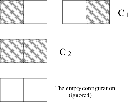
FIG. 1.: Possible occupations of two adjacent sites on an intersection of a DBM structure which is perpendicular to the growth direction. These configurations have probabilities $C_{1}$ and $C_{2}$ as shown.

FIG. 2.: The conditional probability of having a configuration $C_{j}$ above a configuration $C_{i}$ is the FST matrix element $M_{i,j}$. This figure shows a $C_{2}$ configuration at the $k$’th row. The probability for having a $C_{1}$ configuration right above it is $M_{2,1}$.

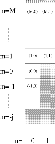
FIG. 3.: The coordinates $(m,n)$ describe the location on a lattice which is 2 sites wide. The grey sites belong to the interface of the aggregate which is shaped as a step whose size is $j$.

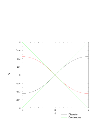
FIG. 4.: The dispersion relations for the discrete and continuous Laplace equation in 2D. The solid line shows the discrete relation $\sinh(\kappa/2)=\pm\sin(k/2)$, and the dashed line shows the continuous relation $\kappa=\pm k$.

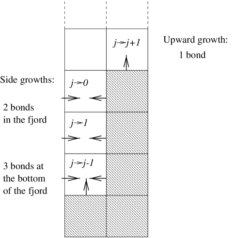
FIG. 5.: Possible growth processes which change the interface from an initial step size $j=3$ to a final size $i=4,0,1,2$. The growth probability is determined by the potential and the number of bonds associated with the site where growth is to occur.

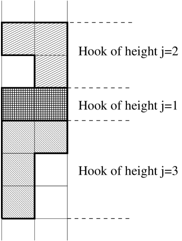
FIG. 6.: The frozen structure behind the interface, composed of hook shaped sub-structures which are laid one on top of the other.

TABLE I.: A summary of our results vs. the FST results and results obtained from simulations

Method	Fractal dimension $D$	Ref.
Our scheme	1.5538	Present
$2\times\infty$ Simulation	1.554	-”-
FST closed scheme	1.55	[10]
FST with
empty configurations
closed scheme	1.4655	[13]
Radial simulation	1.715	[7], [12]
Cylindrical simulation	1.60-66	[8], [12]

TABLE II.: The first 9 components of the steady state vector

$j$	0	1	2	3	4	5	6	7	8
$P_{j}$	.2696	.3113	.1809	.1032	.0586	.0332	.0188	.0106	.0060

TABLE III.: $q(j)$, the exact probability for having a hook which is $j$ sites tall, compared with the relative number of hooks, $\tilde{q}(j)$, in a DLA computer simulation.

$j$	1	2	3	4	5	6	7	8
$q(j)$	.5084	.2117	.1213	.0688	.0390	.0221	.0125	.0071
$\tilde{q}(j)$	.5103	.2127	.1196	.0676	.0391	.0225	.0123	.0074

TABLE IV.: The fractal dimension for different values of $\eta$ - a comparison of our approach to FST (calculated up to two growth processes). The convergence of the calculation goes like $E_{\infty+1,\infty}^{l}$, where $l$ is the order of truncation.

$\eta$	0	0.5	1	2	3	$\infty$
$D$	1.9144	1.7723	1.5538	1.2021	1.07	1
$D_{\rm FST}$	1.8990	1.7515	1.5418	1.1997	-	1
$E_{\infty+1,\infty}$	0	0.3128	0.5658	0.8547	0.96	1