Magnetization Plateaux in $N$-Leg Spin Ladders

Abstract

In this paper we continue and extend a systematic study of plateaux in magnetization curves of antiferromagnetic Heisenberg spin-$1/2$ ladders. We first review a bosonic field-theoretical formulation of a single XXZ-chain in the presence of a magnetic field, which is then used for an Abelian bosonization analysis of $N$ weakly coupled chains. Predictions for the universality classes of the phase transitions at the plateaux boundaries are obtained in addition to a quantization condition for the value of the magnetization on a plateau. These results are complemented by and checked against strong-coupling expansions. Finally, we analyze the strong-coupling effective Hamiltonian for an odd number $N$ of cylindrically coupled chains numerically. For $N=3$ we explicitly observe a spin-gap with a massive spinon-type fundamental excitation and obtain indications that this gap probably survives the limit $N\to\infty$.

I Introduction

So-called “spin ladders” have recently attracted a considerable amount of attention (for reviews see e.g. [1]). They consist of coupled one-dimensional chains and may be regarded as interpolating truly one- and two-dimensional systems. Such an intermediate situation may be useful (among others) for the understanding of high-$T_{c}$ superconductors. In fact, modifications of the high-$T_{c}$ materials (see e.g. [2]) give rise to experimental realizations of spin ladders. However, the field was motivated by an observation that mainly concerns the magnetic spin degrees of freedom, namely the appearance of a spin gap in $N=2$ coupled gapless chains (see e.g. [3]).

One-dimensional quantum magnets have been studied in great detail over the past decades. One remarkable observation in this area is the so-called “Haldane conjecture” [4] which states that isotropic half-integer spin Heisenberg chains are gapless while those with integer spin are gapped. Although this statement has not been proven rigorously yet, a wealth of evidence supporting this conjecture has accumulated in the meantime [5] (see also [6] for a recent field theoretical treatment).

Spin ladders are more general quasi one-dimensional quantum magnets. Again, one of the attractions is a natural generalization of Haldane’s conjecture [4] to such $N$ coupled spin-$S$ chains: If $SN$ is an integer, one expects a gap in zero field, otherwise not. This conjecture is suggested among others by the large-$S$ limit (see [7] for a recent review and references therein), strong-coupling considerations [3, 8], numerical computations [9, 10, 11] and even experiments (see e.g. [2]) . If one includes a strong magnetic field, these Haldane gaps become just a special case of plateaux in magnetization curves. In the presence of a magnetic field, one of the central issues is the quantization condition on the magnetization $\langle M\rangle$ for the appearance of such plateaux, which for the purposes of the present paper will be some special form of

$$lSN(1-\langle M\rangle)\in\hbox{\amsmath Z}\,.$$ (1.1)

Here $\langle M\rangle$ is normalized to a saturation value $\langle M\rangle=\pm 1$ and $l$ is the number of lattice sites to which translational symmetry is either spontaneously or explicitly broken. Haldane’s original conjecture [4] is related to $l=N=1$, $\langle M\rangle=0$. More general cases for $N=1$ were treated in [12, 13, 14]. In an earlier paper [15], we have studied realizations of the condition (1.1) for $N>1$ but with the specializations $l=1$ and $S=1/2$.

So far, spin ladders in strong magnetic fields have attracted surprisingly little attention: To our knowledge, only the case of an $N=2$ leg ladder had been investigated prior to [15]. The experimental measurement of the magnetization curve of the organic two-leg ladder material Cu₂(C₅H₁₂N₂)₂Cl₄ [16] gave rise to theoretical studies using numerical diagonalization [17], series expansions [18] and a bosonic field theory approach [19]. In this case, (i.e. $N=2$ and $S=1/2$) there is a spin gap which gives rise to an $\langle M\rangle=0$ plateau in the magnetization curve. The transition between this zero magnetization plateaux and saturation is smooth and no non-trivial effects (in particular no symmetry breaking) were observed.

For $N>2$ one can expect plateaux at non-trivial $N$-dependent fractions of the saturation magnetization [15]. Though this was a new observation for spin ladders, the phenomenon itself is not completely new. For example, the possibility of magnetization plateaux for the case of single spin-$S$ Heisenberg chains has been discussed systematically in [12] which also motivated some of our work. The attraction of this phenomenon in spin ladders is that they provide clear and natural realizations of such plateaux. For example a numerical analysis of the case $N=3$ explicitly exhibits a robust plateau with $\langle M\rangle=1/3$ [15] which should also be observable experimentally, e.g. in a suitable organic spin-ladder material.

It is the purpose of the present paper to continue a systematic study of (1.1) for generic $N\geq 1$ by using different complementary techniques, such as Abelian bosonization, strong coupling expansions, and numerical computations (the reader may find e.g. [15] helpful in the understanding of the present work). Here, we will among others provide evidence that for $S=1/2$ spontaneous breaking of the translational symmetry to $l=2$ can be induced by strong frustration or an Ising-like anisotropy, while $l\geq 3$ presumably needs explicit symmetry breaking. (In [14] a slightly different example of spontaneous symmetry breaking with $l=2$ was studied).

The prefactor $lSN$ in (1.1) may seem quite cumbersome, but it just counts the possible $S^{z}$-values in a unit cell of a one-dimensional translationally invariant groundstate. It should also be noted that (1.1) is just a necessary condition; whether a plateau actually appears or not depends on the parameters and the details of the model under consideration. For example, plateaux with non-zero $\langle M\rangle\neq 0$ have not been observed in the $SU(2)$ symmetric higher spin-$S$ Heisenberg chains (see e.g. [20]), unless translational invariance is explicitly broken (c.f. [13] for $S=1$).

Conditions of the type (1.1) occur also in generalizations of the Lieb-Schultz-Mattis theorem [21, 22, 23, 12]. This theorem constructs a non-magnetic excitation which in the thermodynamic limit is degenerate with the groundstate for a given magnetization $\langle M\rangle$ and orthogonal to it unless $\langle M\rangle$ satisfies (1.1). In this manner one proves the existence of either gapless excitations or spontaneous breaking of translational symmetry. Unfortunately it is at present not clear that this theorem applies to plateaux in magnetization curves since they require a gap to magnetic excitations.

Here we concentrate mainly on the case $S=1/2$ and all couplings in the antiferromagnetic regimes, but try to keep $N$ as general as possible. Other situations can be analyzed as well, but may lead to somewhat different physics (compare e.g. [24] for the example of $N=3$ antiferromagnetically coupled ferromagnetic chains).

This paper is organized as follows: In section II we first review some aspects of the formulation of a single XXZ-chain as a bosonic $c=1$ conformal field theory. This serves as a basis of later investigations and illustrates some generic features also present in $N$-leg spin ladders. In section III we first introduce the precise lattice model and its field-theoretic counterpart which we then analyze in the weak-coupling regime. Section IV starts from the other extreme –the strong-coupling limit– and proceeds with series expansions around this limit. In section V we discuss an effective Hamiltonian for the strong-coupling limit of an odd number $N$ of cylindrically coupled chains which we then analyze numerically in section VI. We summarize our results by presenting “magnetic phase diagrams” in section VII before we conclude with some comments and open problems (section VIII).

II A single XXZ-chain

First, we recall some results for the XXZ-chain on a ring of $L$ sites in the presence of a magnetic field $h$ applied along the $z$-axis:

$$H_{XXZ}=J\sum_{x=1}^{L}\left\{\Delta S^{z}_{x}S^{z}_{x+1}+{1\over 2}\left(S^{+}_{x}S^{-}_{x+1}+S^{-}_{x}S^{+}_{x+1}\right)\right\}-h\sum_{x=1}^{L}S^{z}_{x}\,.$$ (2.1)

Apart from being the basis for the investigation in later sections, this also serves as an illustration of some general features. It should be noted that in (2.1) the magnetic field is coupled to a conserved quantity which is related to the magnetization $\langle M\rangle$ via $\langle M\rangle=\left\langle{2\over L}\sum_{x=1}^{L}S^{z}_{x}\right\rangle$. For this reason, properties of (2.1) in the presence of a magnetic field $h\neq 0$ can be related to those at $h=0$ and the magnetic field $h$ can be considered as a chemical potential.

The Hamiltonian (2.1) is exactly solvable by Bethe ansatz also for $h\neq 0$. In this way it can be rigorously shown that its low-energy properties are described by a $c=1$ conformal field theory of a free bosonic field compactified at radius $R$ in the thermodynamic limit for $\Delta>-1$ and any given magnetization $\langle M\rangle$ (see e.g. [25] and compare also [26] for a detailed discussion of the case $|\Delta|<1$). More precisely, upon insertion of the bosonized representation of the spin operators into the Hamiltonian (2.1) (see e.g. [27]) one obtains the following low-energy effective Hamiltonian for the XXZ-chain:

$$\bar{H}_{XXZ}=\int{\rm d}x{\pi\over 2}\left\{\Pi^{2}(x)+R^{2}(\langle M\rangle,\Delta)\left(\partial_{x}\phi(x)\right)^{2}\right\}$$ (2.2)

with $\Pi={1\over\pi}\partial_{x}\tilde{\phi}$, and $\phi=\phi_{L}+\phi_{R}$, $\tilde{\phi}=\phi_{L}-\phi_{R}$. In (2.2) we have suppressed a for our purposes irrelevant proportionality constant that includes the velocity of sound. In this formulation, the effect of both the magnetic field $h$ and XXZ-anisotropy $\Delta$ turns up only via the radius of compactification $R(\langle M\rangle,\Delta)$. This radius governs the conformal dimensions, in particular the conformal dimension of a vertex operator ${\rm e}^{i\beta\phi}$ is given by $\left({\beta\over 4\pi R}\right)^{2}$. We now describe how $R$ can be computed.

We parametrize the XXZ-anisotropy by $\Delta=\cos\theta$ with $0<\theta<\pi$ for $-1<\Delta<1$ and by $\Delta=\cosh\gamma$ with $\gamma>0$ for $\Delta>1$. Now for given magnetization $\langle M\rangle\geq 0$ and XXZ-anisotropy $\Delta$, the associated radius of compactification $R$ and magnetic field $h/J$ can be obtained by solving integral equations (see e.g. [26, 28, 29, 30]) in the following way: Firstly, introduce a function $\sigma(\eta)$ for the density of particles satisfying the integral equation

$$\sigma(\eta)={1\over 2\pi}\left\{g(\eta)-\int_{-\Lambda}^{\Lambda}K(\eta-\eta^{\prime})\sigma(\eta^{\prime}){\rm d}\eta^{\prime}\right\}$$ (2.3)

where the kernel $K(\eta)$ and the righthand side $g(\eta)$ are presented in Table I.

$\Delta$	$K(\eta)$	$g(\eta)$	$\epsilon_{0}(\eta)$
$\cos\theta=\Delta<1$	${\tan\theta\over\tan^{2}\theta\;\cosh^{2}{\eta\over 2}+\sinh^{2}{\eta\over 2}}$	${\cot{\theta\over 2}\over\cosh^{2}{\eta\over 2}+\cot^{2}{\theta\over 2}\;\sinh^{2}{\eta\over 2}}$	${h\over J}-{\sin^{2}{\theta}\over\cosh{\eta}-\cos{\theta}}$
$\Delta=1$	${4\over\eta^{2}+4}$	${2\over\eta^{2}+1}$	${h\over J}-{2\over\eta^{2}+1}$
$\cosh\gamma=\Delta>1$	${\tanh\gamma\over\tanh^{2}\gamma\;\cos^{2}{\eta\over 2}+\sin^{2}{\eta\over 2}}$	${\coth{\gamma\over 2}\over\cos^{2}{\eta\over 2}+\coth^{2}{\gamma\over 2}\;\sin^{2}{\eta\over 2}}$	${h\over J}-{\sinh^{2}{\gamma}\over\cos{\eta}-\cosh{\gamma}}$

TABLE I.: Functions appearing in the integral equations.

The real parameter $\Lambda\geq 0$ in (2.3) describes the spectral parameter value at the Fermi surface and is determined by the magnetization $\langle M\rangle$ via the filling condition

$$\int_{-\Lambda}^{\Lambda}\sigma(\eta){\rm d}\eta={1\over 2}\left(1-\langle M\rangle\right)\,.$$ (2.4)

In general, one has to adjust $\Lambda$ iteratively by first numerically solving (2.3) and then checking for (2.4). Only some special cases can be solved explicitly. This includes the case $\langle M\rangle=0$ and $\Delta\leq 1$ where $\Lambda=\infty$ is the correct choice. Once the desired value of $\Lambda$ is determined, one introduces a dressed charge function $\xi(\eta)$ (see e.g. [28, 29]) as a solution of the integral equation

$$\xi(\eta)=1-{1\over 2\pi}\int_{-\Lambda}^{\Lambda}K(\eta-\eta^{\prime})\xi(\eta^{\prime}){\rm d}\eta^{\prime}$$ (2.5)

giving directly rise to the radius of compactification

$$R(\langle M\rangle,\Delta)={1\over\sqrt{4\pi}\;\xi(\Lambda)}\,.$$ (2.6)

If one further wants to determine the associated magnetic field $h$, one has to introduce another function $\epsilon_{d}(\eta)$, the dressed energy, satisfying the integral equation

$$\epsilon_{d}(\eta)=\epsilon_{0}(\eta)-{1\over 2\pi}\int_{-\Lambda}^{\Lambda}K(\eta-\eta^{\prime})\epsilon_{d}(\eta^{\prime}){\rm d}\eta^{\prime}$$ (2.7)

with the bare energy $\epsilon_{0}(\eta)$ listed in Table I. Then the magnetic field $h/J$ is determined by the condition that the energy of the dressed excitations vanishes at the Fermi surface

$$\epsilon_{d}(\Lambda)=0\,.$$ (2.8)

Using (2.5) one can see that $\epsilon(\eta)=\epsilon(\eta)|_{h=0}+{h\over J}\xi(\eta)$ solves (2.7) if $\epsilon(\eta)|_{h=0}$ solves (2.7) with formally $h=0$ (but for the given $\langle M\rangle$). From this and (2.8) one can easily obtain $h$ once $\Lambda$ is known via $h/J=-\epsilon(\Lambda)|_{h=0}/\xi(\Lambda)$.

In general, these integral equations have to be solved numerically and $\Lambda$ has to be determined by some iterative method. Although this is readily done by standard methods, a generally accessible implementation seems to be still unavailable. We have therefore decided to tentatively provide access to such solutions on the WWW [31]. This implementation works in the way described above. Typically, it gives results with an absolute accuracy of $10^{-6}$ or better. Of course, one can change the order of the procedure: For example one could also prescribe $h/J$, then determine $\Lambda$ from (2.7) and (2.8), next the radius of compactification $R$ from (2.5) and (2.6) and finally (optionally) the magnetization $\langle M\rangle$ from (2.3) and (2.4).

Some remarks are in order concerning the case $\Delta>1$: In this region the identification with a $c=1$ conformal field theory has been established directly only by a numerical analysis of the Bethe-ansatz equations (for a summary see e.g. section 2 of [32]). However, the six-vertex model in external fields has been shown [33] to yield a $c=1$ conformal field theory, and since the XXZ-chain arises as the Hamiltonian limit of the six-vertex model, this indirectly establishes the identification. Still, explicit formulae e.g. for $R$ are not available in the literature and therefore we have obtained the integral equations presented for the case $\Delta>1$ above by an analytical continuation of those for $\Delta<1$, as is suggested e.g. by [34] (see also [35] – apparently such a continuation was also used in the recent work [13]). We have performed some checks that this yields indeed correct results. For example, some radii $R$ associated to certain magnetic fields $h$ and anisotropies $\Delta$ obtained numerically for chains of length up to $L=234$ [36] are reproduced in this way.

As a further check, one can compare the critical magnetic field for the boundary of the $\langle M\rangle=0$ plateau at $\Delta>1$ obtained by numerical solution of the above integral equations with the exact solution of the Bethe-ansatz equations [37]

$${h_{c}\over J}={2\pi\sinh{\gamma}\over\gamma}\sum_{n=0}^{\infty}{1\over\cosh{{(2n+1)\pi^{2}\over 2\gamma}}}\,,$$ (2.9)

where as before $\Delta=\cosh{\gamma}$. In this case (i.e. for $\langle M\rangle=0$) one has $\Lambda=\pi$ and the above integral equations can be solved using Fourier series [34, 35, 37]. If one solves the above integral equations numerically, the deviation from the exact result (2.9) is of the order of the numerical accuracy (in our implementation [31] always less than $10^{-6}$).

In passing we make a comment which will turn out to be useful later. The result (2.9) is the gap to $S^{z}=1$ excitations. However, the fundamental excitation of the XXZ-chain is known to be a so-called “spinon” which carries $S^{z}=1/2$ [38, 39, 40]. This spinon can be regarded as a domain-wall between the two antiferromagnetic groundstates for $\Delta>1$. Since a single spin-flip creates two domain-walls, the lowest $S^{z}=1$ excitation is a scattering state of two spinons. This picture can be useful e.g. in numerical computations. For example, a single spinon can be observed for odd $L$ with periodic boundary conditions.

After this digression let us now return to the above integral equations. The results obtained from them are summarized in the magnetic phase diagram for the XXZ-chain Fig. 1 (see also [41, 32] for similar pictures). There are two gapped phases: A ferromagnetic one at sufficiently strong fields (which is actually the only one for $\Delta<-1$) and an antiferromagnetic phase for $\Delta>1$ at small fields. In between is the massless phase where the bosonized form (2.2) is valid. An elementary computation of the spinwave dispersion above the ferromagnetic groundstate shows that the transition between the ferromagnetic phase and the massless phase is located at $h/J=1+\Delta$. This transition is a very clear example of the DN-PT universality class [42, 43] , i.e. for $\langle M\rangle\to 1$ the magnetization behaves as (compare also [44])

$$\left(\langle M\rangle-M_{c}\right)^{2}\sim h^{2}-h_{c}^{2}$$ (2.10)

with here $M_{c}=1$ and $h_{c}/J=1+\Delta$. At this transition the radius takes the universal value $R(1,\Delta)={1\over 2\sqrt{\pi}}$.

FIG. 1.: Magnetic phase diagram of the XXZ-chain (2.1). For explanations compare the text.

The other transition line starts at the $SU(2)$ symmetric point $\langle M\rangle=0$, $\Delta=1$ with a radius $R(0,1)={1\over\sqrt{2\pi}}$. Actually, at $\langle M\rangle=0$ the additional operator

$$\cos\left(4\sqrt{\pi}\phi\right)$$ (2.11)

appears in the continuum limit, which we have suppressed in (2.2) since it is irrelevant inside the massless phase. At $\Delta=1$ it is marginal and becomes relevant for $\Delta>1$, opening the gap that gives the boundary of the antiferromagnetic phase in Fig. 1. The associated phase transition is a Kosterlitz-Thouless (K-T) transition [45] (see e.g. [46, 47, 48]). The almost marginal nature of the operator responsible for the gap leads to a stretched exponential decay for $\Delta$ slightly bigger than one which is characteristic for a K-T transition [49]. The exact asymptotic form for the gap (or critical magnetic field) of the XXZ-chain is easily obtained from the Bethe-ansatz solution (2.9) upon noting that $\gamma\approx\sqrt{2(\Delta-1)}$ and that in the limit $\Delta\to 1$ only the term $n=0$ contributes to the sum. One then finds [37]:

$$\qquad\qquad{h_{c}\over J}\sim 4\pi{\rm e}^{-{\pi^{2}\over 2\sqrt{2(\Delta-1)}}}\qquad\qquad\hbox{(for $\Delta$ slightly bigger than $1$).}$$ (2.12)

For this reason the phase boundary is indistinguishable from the $h=0$ line for XXZ-anisotropies up to $\Delta\approx 1.2$ on the scale of Fig. 1. In this region, the numerical determination of the radius $R$ is difficult for $\langle M\rangle\to 0$. Nevertheless, using that $\Lambda=\pi$ for $\langle M\rangle=0$ and $\Delta>1$, one can readily check that the constant function $\xi(\eta)={1\over 2}$ solves the integral equation (2.5). Then one obtains from (2.6) that $R(0,\Delta>1)={1\over\sqrt{\pi}}$.

For $\langle M\rangle=0$ and $|\Delta|\leq 1$ one has $\Lambda=\infty$ (see above) and one can use the Wiener-Hopf method to solve the above integral equations in closed form. This yields in particular $R(0,\Delta)=\sqrt{{1\over 2\pi}\left(1-{1\over\pi}\cos^{-1}\Delta\right)}$ [27]. In general, the radius $R$ increases with increasing $\Delta$. For $\Delta>0$, it decreases with increasing magnetization $\langle M\rangle$, while for $\Delta<0$ this is reversed to an increase in $R$ with increasing $\langle M\rangle$. Clearly, the radius must be constant on the XY-line which separates these two regions: $R(\langle M\rangle,0)={1\over 2\sqrt{\pi}}$ (though the magnetic field associated to a given $\langle M\rangle$ is still a non-trivial function which should be computed from the above integral equations).

FIG. 2.: Magnetization curve of the XXZ-chain at $\Delta=2$ obtained from the integral equations (2.3), (2.4), (2.7) and (2.8). The inset shows the region of small magnetization and illustrates that also the transition $\langle M\rangle\to 0$ is compatible with the DN-PT universality class for $\Delta>1$ (the dashed line is a fit to the universal form (2.10)).

Including the operator (2.11) in the bosonized language (2.2), one recovers a Hamiltonian treated in [50] as a model for commensurate-incommensurate transitions. This means that the transition $\langle M\rangle\to 0$ for $\Delta>1$ is predicted to be in the DN-PT universality class [42, 43], too. The same bosonization argument also leads to the already mentioned result $R(0,\Delta>1)={1\over\sqrt{\pi}}$ (see also [25]). The inset in Fig. 2 illustrates for $\Delta=2$ that for sufficiently small magnetizations one can indeed observe a behaviour that is compatible with the universal square-root (2.10). It should be noted though that the window for the universal DN-PT behaviour is too small to permit verification within our numerical accuracy for smaller values of $\Delta$ (e.g. $\Delta\leq 1.2$) where neither a reliable numerical check of the result $R={1\over\sqrt{\pi}}$ is possible. An analytic check of the asymptotic behaviour of the magnetization from the Bethe-ansatz solution would be interesting, but is beyond the scope of the present paper.

It should be noted that the height of the entire inset in Fig. 2 corresponds to the first step in the magnetization curve of a chain of the finite size $L=112$. Therefore, the exact solution is crucial in verifying the exponent (2.10) – a numerical or experimental verification of this behaviour restricted to such a small region would be extremely difficult. Similar difficulties will be faced in an experimental or numerical verification of $R(0,\Delta)={1\over\sqrt{\pi}}$ or the equivalent statement for the correlation function exponents in the region of $\Delta$ slightly larger than 1.

III Ladders: Weak coupling and Abelian bosonization

In this section we apply Abelian bosonization to the weak-coupling region ${J^{\prime}}\ll J$ of $N$-leg spin ladders. In particular, we will show how the necessary condition (1.1) arises in this formulation and discuss under which circumstances an allowed plateau does indeed open as a function of the parameters ${J^{\prime}}$ and $\Delta$. The lattice Hamiltonian for this system is given by

$$H^{(N)}={J^{\prime}}\sum_{i,j}\sum_{x=1}^{L}\vec{S}_{i,x}\vec{S}_{j,x}+J\sum_{i=1}^{N}\sum_{x=1}^{L}\left\{\Delta S^{z}_{i,x}S^{z}_{i,x+1}+{1\over 2}\left(S^{+}_{i,x}S^{-}_{i,x+1}+S^{-}_{i,x}S^{+}_{i,x+1}\right)\right\}-h\sum_{i,x}S^{z}_{i,x}\,,$$ (3.1)

where ${J^{\prime}}$ and $J$ are respectively the interchain and intrachain couplings, $h$ is the external magnetic field and the indices $i$ and $j$ label the different chains (legs) in the ladder. The sum in the first term is over all possible couplings between chains. The case of periodic boundary conditions (PBC) and open boundary conditions (OBC) will be discussed later. Here we have explicitly included an XXZ-anisotropy $\Delta$ in the intrachain coupling. We have kept the interchain coupling ${J^{\prime}}$ $SU(2)$ symmetric for simplicity in later sections although this is not substantial in the weak-coupling region which we will discuss in the remainder of this section.

The corresponding effective field-theoretic Hamiltonian is obtained using standard methods [51, 27] (see also [12, 13, 14] for the case of non-zero magnetization). One essentially uses (2.2) as the effective Hamiltonian for each chain and the bosonized expressions for the spin operators which read:

$$S^{z}_{i,x}\approx\frac{1}{\sqrt{2\pi}}\frac{\partial\phi_{i}}{\partial x}+const.:\cos(2k_{F}^{i}x+\sqrt{4\pi}\phi_{i}):+{\langle M_{i}\rangle\over 2}\,,$$ (3.2)

and

$$S^{\pm}_{i,x}\approx\ :{\rm e}^{\pm i\sqrt{\pi}\tilde{\phi}_{i}}(1+const.\cos(2k_{F}^{i}x+\sqrt{4\pi}\phi_{i})):\,.$$ (3.3)

Here we have set a lattice constant to unity which appears in passing to the continuum limit. The colons denote normal ordering which we take with respect to the groundstate of a given mean magnetization $\langle M_{i}\rangle$ in the $i$th chain which is a natural choice. This leads to the constant term in (3.2) which will play an important rôle in the discussion of the terms that can be generated radiatively. The prefactor $1/2$ arises from our normalization of the magnetization to saturation values $\langle M\rangle=\pm 1$. The Fermi momenta $k_{F}^{i}$ are given by $k_{F}^{i}=\pi(1-\langle M_{i}\rangle)/2$.

In the weak-coupling limit along the rungs, ${J^{\prime}}\ll J$, we obtain the following bosonized low-energy effective Hamiltonian for the $N$-leg ladder keeping only the most relevant perturbation terms:

$$\bar{H}^{(N)} = \int{\rm d}x\Biggl{[}{\pi\over 2}\sum_{i=1}^{N}\left\{\Pi_{i}^{2}(x)+R^{2}(\langle M\rangle,\Delta)\left(\partial_{x}\phi_{i}(x)\right)^{2}\right\}$$ (3.4)

$$+ {\lambda_{1}\over 2\pi}\sum_{i,j}\left(\partial_{x}\phi_{i}(x)\right)\left(\partial_{x}\phi_{j}(x)\right)$$ (3.5)

$$+ \sum_{i,j}\biggl{\{}\lambda_{2}:\cos(2x(k_{F}^{i}+k_{F}^{j})+\sqrt{4\pi}(\phi_{i}+\phi_{j})):$$ (3.7)

$$\!\!\!+\lambda_{3}:\cos(2x(k_{F}^{i}-k_{F}^{j})+\sqrt{4\pi}(\phi_{i}-\phi_{j})):+\lambda_{4}:\cos\left(\!\sqrt{\pi}(\tilde{\phi}_{i}-\tilde{\phi}_{j})\!\right)\!:\biggr{\}}\Biggr{]}\,,$$

The four coupling constants $\lambda_{i}$ essentially correspond to the coupling ${J^{\prime}}$ between the chains: $\lambda_{i}\sim{J^{\prime}}/J$. In arriving to the Hamiltonian (3.7) we have discarded a constant term and absorbed a term linear in the derivatives of the free bosons into a redefinition of the applied magnetic field.

The Hamiltonian (3.7) has been also used to represent spin-$N/2$ chains (see e.g. [51, 52]), since they can be obtained in the limit of $N$ strongly ferromagnetically coupled chains (${J^{\prime}}\to-\infty$). However, here we will analyze (3.7) mainly in the case of small antiferromagntic ${J^{\prime}}$ and discuss various boundary conditions.

Note that the $\lambda_{2}$ and $\lambda_{3}$ perturbation terms contain an explicit dependence on the position (in the latter case this $x$-dependence disappears for symmetric configurations with equal $k_{F}^{i}$). Such operators survive in passing from the lattice to the continuum model, assuming that the fields vary slowly, only when they are commensurate. In particular, the $\lambda_{2}$ term appears in the continuum limit only if the oscillating factor $\exp(i2x(k_{F}^{i}+k_{F}^{j}))$ equals unity. If the configuration is symmetric, this in turn happens only for zero magnetization (apart from the trivial case of saturation).

For simplicity let us first analyze the case with $N=3$ and PBC. We first have to diagonalize the Gaussian (derivative) part of the Hamiltonian. This is achieved by the following change of variables in the fields:

$$\psi_{1}={1\over\sqrt{2}}\left(\phi_{1}-\phi_{3}\right)\,,\qquad\psi_{2}={1\over\sqrt{6}}\left(\phi_{1}+\phi_{3}-2\phi_{2}\right)\,,\qquad\psi_{D}={1\over\sqrt{3}}\left(\phi_{1}+\phi_{2}+\phi_{3}\right)\,.$$ (3.8)

In terms of these fields the derivative part of the Hamiltonian can be written as:

$$\bar{H}_{{\rm der.}}=\int{\rm d}x{\pi\over 2}\left\{R^{2}(\langle M\rangle,\Delta)\left[(1+a)\left(\partial_{x}\psi_{D}(x)\right)^{2}+(1-b)\left(\left(\partial_{x}\psi_{1}(x)\right)^{2}+\left(\partial_{x}\psi_{2}(x)\right)^{2}\right)\right]\right\}$$ (3.9)

where $a=2{J^{\prime}}/(J\pi^{2}R^{2})=2b$. We can now study the large-scale behaviour of the effective Hamiltonian (3.7) where we assume all $k_{F}^{i}$ equal due to the symmetry of the chosen configuration of couplings. Let us first consider the case when the magnetization $\langle M\rangle$ is non-zero. In this case only the $\lambda_{3}$ and $\lambda_{4}$ terms are present. The one-loop R.G. equations are:

$$\frac{db}{d\ln{L}} = 4\pi\left(-\frac{3\lambda_{3}^{2}}{2R^{2}}+12\pi^{2}R^{2}\lambda_{4}^{2}\right)$$ (3.10)

$$\frac{d\lambda_{3}}{d\ln{L}} = \left(2-\frac{1}{2\pi R^{2}(1-b)}\right)\lambda_{3}-\pi\lambda_{3}^{2}$$ (3.11)

$$\frac{d\lambda_{4}}{d\ln{L}} = \left(2-2\pi R^{2}(1-b)\right)\lambda_{4}-\pi\lambda_{4}^{2}\,.$$ (3.12)

It is important to notice that only the fields $\psi_{1}$ and $\psi_{2}$ enter in these R.G. equations, since the perturbing operators do not contain the field $\psi_{D}$. The behaviour of these R.G. equations depends on the value of $R$. The main point is that always one of the two $\lambda$ perturbation terms will dominate and the corresponding cosine operator tends to order the associated fields. This gives a finite correlation length in correlation functions containing the fields $\psi_{1}$ and $\psi_{2}$ (or their duals). For example, for $\Delta\leq 1$ we have that $R^{2}<(2\pi)^{-1}$ since $\langle M\rangle\neq 0$. Then, from (3.12) one can easily see that the dominant term will be the $\lambda_{4}$ one. This term orders the dual fields associated with $\psi_{1}$ and $\psi_{2}$. Then, the correlation functions involving these last fields decay exponentially to zero. In either case, the field $\psi_{D}$ remains massless. A more careful analysis of the original Hamiltonian shows that this diagonal field will be coupled to the massive ones only through very irrelevant operators giving rise to a renormalization of its compactification radius. However, due to the strong irrelevance of such coupling terms these corrections to the radius are expected to be small, implying that the value of the large-scale effective radius keeps close to the zero-loop result $R\sqrt{1-a}$. It is straightforward to generalize this to $N$ chains when all possible coupling are present and have the same value ${J^{\prime}}$. One can find a change of variables on the fields to:

$$\psi_{D}~{}~{};~{}~{}\psi_{i}~{}~{}~{}i=1,\ldots,N-1$$

where $\psi_{D}={1/\sqrt{N}}\sum_{i=1}^{N}\phi_{i}$. Again, for non-zero magnetization, all but the diagonal field $\psi_{D}$ will be present in the perturbing terms $\lambda_{3}$ and $\lambda_{4}$. The R.G. equations are essentially the same as (3.12) and the result is that only the field $\psi_{D}$ will be massless.

We are then left in principle with a free Gaussian action for the diagonal field. However some operators can be radiatively generated. We see from eqs. (3.2,3.3) that when we turn on the interchain coupling, the “N-Umklapp” term

$${J^{\prime}}^{N}\cos\left(2x\sum_{i=1}^{N}k_{F}^{i}+\sqrt{4\pi}\sum_{i=1}^{N}\phi_{i}\right)={J^{\prime}}^{N}\cos\left(2x\sum_{i=1}^{N}k_{F}^{i}+\sqrt{4\pi N}\psi_{D}\right)$$ (3.13)

appears in the operator product expansion (OPE).

Again, this operator survives in passing from the lattice to the continuum model, assuming that the fields vary slowly, only when the oscillating factor $\exp(i2x\sum_{j=1}^{N}k_{F}^{j})$ equals one. This in turn will happen when the following specialized version of the condition (1.1)

$${N\over 2}(1-\langle M\rangle)\in\hbox{\amsmath Z}\,$$ (3.14)

is satisfied. At such values of the magnetization, the field $\psi_{D}$ can then undergo a K-T transition to a massive phase, indicating the presence of a plateau in the magnetization curve. An estimate of the value of ${J^{\prime}}$ at which this operator becomes relevant can be obtained from its scaling dimension which in zero-loop approximation is given by

$$\dim\left(\cos\left(\sqrt{4\pi N}\psi_{D}\right)\right)={N\over 4\left(\pi R^{2}+{N-1\over\pi}\;{{J^{\prime}}\over J}\right)}\,.$$ (3.15)

At $\Delta=1$ one then obtains ${J^{\prime}_{c}}\approx 0.09J$ for the $\langle M\rangle=1/3$ plateau at $N=3$ and ${J^{\prime}_{c}}\approx 0.7J$ for $\langle M\rangle=1/2$ at $N=4$ and also for $\langle M\rangle=1/5$ at $N=5$. At the opening of such plateaux, the effective radius of compactification is fixed to be:

$$R_{{\rm eff.}}^{2}={N\over 8\pi}$$ (3.16)

and the large-scale effective spin operators are (c.f. [51]):

$$S^{z}_{{\rm eff.}}(x)\approx\sqrt{{N\over 2\pi}}\frac{\partial\psi_{D}}{\partial x}+const.:\cos(2k_{F}x+\sqrt{4\pi N}\psi_{D}):+{\langle M\rangle\over 2}\,,$$ (3.17)

and

$$S^{\pm}_{{\rm eff.}}(x)\approx\ :{\rm e}^{\pm i\sqrt{\pi/N}\tilde{\psi}_{D}}(1+const.\cos(2k_{F}x+\sqrt{4\pi N}\psi_{D})):\,.$$ (3.18)

Then, eq. (3.16) fixes the values of the correlation exponents at this point to be

$$\eta_{z}=4\,;\qquad\eta_{xy}={1\over 4}\,.$$ (3.19)

On the other hand, commensurate-incommensurate transition results [50, 19, 13] imply that the values of these exponents should be

$$\eta_{z}=2\,;\qquad\eta_{xy}={1\over 2}$$ (3.20)

along the upper and lower boundary of a plateau. This situation is similar to the XXZ-chain at $\Delta=1$ and $\Delta>1$ for the boundary of the $\langle M\rangle=0$ plateau. However, the values of the exponents are different since the perturbing operators are different.

Note that the “N-Umklapp” process which allows the appearance of (3.13) produces a complete family of operators given by:

$$\cos\left(2xl\sum_{i=1}^{N}k_{F}^{i}+l\sqrt{4\pi}\sum_{i=1}^{N}\phi_{i}\right)=\cos\left(2xl\sum_{i=1}^{N}k_{F}^{i}+l\sqrt{4\pi N}\psi_{D}\right)$$ (3.21)

with $l$ an arbitrary integer. The values of the magnetization for which one of these operators is allowed are subject to a generalization of (3.14), namely (1.1) in the Introduction (with $S=1/2$). However, the dimensions of these operators increase with $l^{2}$. So, these operators cannot be relevant unless we consider regimes with an anisotropy parameter $\Delta$ bigger than one or very big values of the interchain coupling ${J^{\prime}}$ far from the perturbative regime of the present analysis. Therefore, higher values of $l$ are realized only under special conditions. While $l=2$ can be obtained by either strong Ising-like anisotropy $\Delta$ or frustration at strong coupling (see section VI below), it is possible that $l\geq 3$ can be realized only if suitable symmetry breaking terms are explicitly introduced into the Hamiltonian (3.1).

Note that formally, the preceding analysis can also be carried out using the fermionic Jordan-Wigner formulation. For example, in this formulation the “N-Umklapp” operator (3.13) is given by

$$\left(\prod_{a=1}^{N}R_{a}^{\dagger}(x)L_{a}(x)\exp(2ik_{F}^{a}x)\right)+\left(\prod_{a=1}^{N}L_{a}^{\dagger}(x)R_{a}(x)\exp(-2ik_{F}^{a}x)\right)\,,$$

where $R_{a}$ and $L_{a}$ are the right- and left-moving components of the fermions. We have chosen to use the bosonized language because it is more appropriate for general values of the anisotropy $\Delta$.

The analysis above was for the case where all the chains were coupled together with the same coupling value. More precisely, the estimates for the appearance of plateaux were for positive (frustrating) interchain coupling. To generalize this to PBC (which is different from the preceding case for $N\geq 4$), we first notice, using the bosonized expression of the effective Hamiltonian, that this configuration of couplings is not stable under R.G. transformation. E.g. the OPE between terms like $\cos(\phi_{1}-\phi_{2})$ and $\cos(\phi_{2}-\phi_{3})$ generates an effective coupling between the fields $\phi_{1}$ and $\phi_{3}$, etc. The underlying intuitive picture is that antiferromagnetic couplings between the chain $2$ with the chains $1$ and $3$ generates an effective ferromagnetic coupling between the chains $1$ and $3$. For example, for $N=4$ and PBC, ferromagnetic couplings are generated along the diagonals between originally uncoupled chains. This case is part of the family of configurations with antiferromagnetic nearest neighbour and ferromagnetic next-nearest neighbour couplings. For this general situation at $N=4$, the coupling matrix in the derivative part is given by:

$$\pmatrix{1&a&-b&a\cr a&1&a&-b\cr-b&a&1&a\cr a&-b&a&1\cr}$$ (3.22)

where $a$ and $b$ are positive. As in the preceding analysis, one can change variables to

$$\displaystyle\psi_{D}={1\over\sqrt{4}}(\phi_{1}+\phi_{2}+\phi_{3}+\phi_{4})\,;\quad \psi_{1}={1\over\sqrt{4}}(\phi_{1}-\phi_{2}+\phi_{3}-\phi_{4})\,;$$ (3.23)

$$\displaystyle\psi_{2}={1\over\sqrt{2}}(\phi_{1}-\phi_{3})\,; \psi_{3}={1\over\sqrt{2}}(\phi_{2}-\phi_{4})\,.$$ (3.24)

For generic values of the magnetization, it is easy to see that the diagonal field $\psi_{D}$ is again the only field that does not acquire a mass under the perturbation. Then, the analysis of the appearance of the N-Umklapp term for particular values of the magnetization is identical to the one performed before. The generalization to generic $N$ with PBC is straightforward, one first builds the radiatively generated couplings by keeping only the lowest order in ${J^{\prime}}$. Once this step is performed, the only difference with respect to the case of equal interchain couplings is the zero-loop value of the dimension of the N-Umklapp operator (which enters via the initial conditions for the R.G. flow). This has the effect of changing the value of the coupling ${J^{\prime}}$ at which a plateau opens with a given value of the magnetization, but the qualitative behaviour of the system is similar. This conclusion is not so straightforward for $\langle M\rangle=0$, where as we will see, the difference between frustrating and non-frustrating configurations can become crucial.

Concerning finally the case of OBC, let us first consider again the case $N=3$ with antiferromagnetic coupling between the first and second chain and the second and the third chain. Again, this coupling is not stable under R.G. transformation. Under R.G. transformations the OBC configuration will flow towards a non-frustrating cyclically coupled configuration. The main point is that for weak coupling and non-zero magnetization, the most relevant perturbing term will be again the one containing differences of fields or their duals. Then they will produce a mass gap for all the relative degrees of freedom and one recovers a scenario similar to the symmetric case, where only one massless field is left. On the other hand, the appearance of “N-Umklapp” operators and their commensurability is unchanged, since these criteria depend on the value of the magnetization and not on the particular couplings between the chains.

Let us study now the more complicated case of zero magnetization. For $\langle M\rangle=0$ the $\lambda_{2}$ term in (3.7) is commensurate and must be included in the perturbation terms. The situation is now much more complicated because this relevant operator couples the diagonal field $\psi_{D}$ with the massive ones. For equal coupling between $N=3$ chains, the R.G. equations are now:

$$\frac{da}{d\ln{L}} = \frac{16\pi\lambda_{2}^{2}}{R^{2}}$$ (3.25)

$$\frac{db}{d\ln{L}} = 4\pi\left(-\frac{\lambda_{2}^{2}}{2R^{2}}-\frac{3\lambda_{3}^{2}}{2R^{2}}+12\pi^{2}R^{2}\lambda_{4}^{2}\right)$$ (3.26)

$$\frac{d\lambda_{2}}{d\ln{L}} = \left(2-\frac{2}{3}\frac{1}{4\pi R^{2}}\left(\frac{2}{1+a}+\frac{1}{1-b}\right)\right)\lambda_{2}-\pi\lambda_{2}\lambda_{3}$$ (3.27)

$$\frac{d\lambda_{3}}{d\ln{L}} = \left(2-\frac{1}{2\pi R^{2}(1-b)}\right)\lambda_{3}-\pi\lambda_{3}^{2}-\pi\lambda_{2}^{2}$$ (3.28)

$$\frac{d\lambda_{4}}{d\ln{L}} = \left(2-2\pi R^{2}(1-b)\right)\lambda_{4}-\pi\lambda_{4}^{2}$$ (3.29)

with the R.G. initial conditions

$$a(0)=2b(0)={2{J^{\prime}}\over J\pi^{2}R^{2}},$$ (3.30)

and

$$\lambda_{2}(0)=\lambda_{3}(0)=1/2(const)^{2}{J^{\prime}}/J~{};~{}\lambda_{4}(0)={J^{\prime}}/J$$ (3.31)

where we kept the notation of (3.7,3.9). We see that the radius of compactification of the diagonal field is now strongly affected by the presence of the $\lambda_{2}$ term. Note also that the “N-Umklapp” process generates the operator

$${J^{\prime}}^{N}\cos\left(\sqrt{4\pi N}\psi_{D}\right)$$ (3.32)

for $N$ even, and

$${J^{\prime}}^{N}\cos\left(2\sqrt{4\pi N}\psi_{D}\right)$$ (3.33)

for $N$ odd. For non-frustrating interchain coupling (a negative ${J^{\prime}}$ coupling between all the chains for example), all relative fields are massive according to [52]. We can then integrate out these massive degrees of freedom. The crucial point is that now the radius of the diagonal field gets a non-trivial correction due to the strong interaction with the massive fields. Since this field is the only one expected to describe the large-scale behaviour of the system, for $\Delta=1$ and $\langle M\rangle=0$, the $SU(2)$ symmetry of the model would fix the radius of this field to be [52]:

$$R_{{\rm eff.}}=\sqrt{N\over{2\pi}}\,.$$ (3.34)

For such a value of the renormalized radius, the “N-Umklapp” term becomes strongly relevant for $N$ even, and marginally irrelevant for $N$ odd. These arguments are based on the assumption that the (uncontrolled) R.G. flow will drive our system to the ($SU(2)$ symmetric) strong coupling regime. The situation is even more subtle for positive ${J^{\prime}}$ (or $\lambda_{i}$), because in this case, from (3.29) one sees that the quadratic terms could now prevent the R.G. flow to reach the same strong coupling regime as for ${J^{\prime}}<0$. A numerical analysis of the R.G. flow for a frustrated three-leg Hubbard ladder at half filling provides evidence for the opening of a gap [53]. On the other hand, a non-abelian bosonization analysis [54] lead to the conclusion that the weak-coupling region is gapless. This case deserves further investigation and series expansions are one way to approach this issue.

IV Strong coupling expansions for $N$-leg ladders

In this section we diagonalize the interaction along the rungs exactly for $J=0$ and then expand quantities of interest in powers of $J/{J^{\prime}}$ around this limit. In order to be able to cover a variety of cases, we used a quite general method to perform the series expansions which is summarized e.g. in section 3 of [55] (actually, the program used in the present paper is a modified version of the one used loc.cit.).

As was already pointed out in [15], one can simply count the number of chains $N$ in the limit $J/{J^{\prime}}\to 0$ in order to determine the allowed values of the magnetization $\langle M\rangle$. This is presumably the simplest way to obtain the quantization condition (3.14). A less trivial fact is that all these values of the magnetization are in fact realized. For example, for ferromagnetic coupling ${J^{\prime}}<0$, the magnetization jumps immediately from one saturated value $\langle M\rangle=-1$ to the other one ($\langle M\rangle=+1$) as the magnetic field $h$ passes through zero. Nevertheless, for not too large $N$ one can readily compute the magnetization curve of (2.1) and check for antiferromagnetic coupling ${J^{\prime}}>0$ that all possible values of the magnetization are indeed successively realized as the field is increased. The critical magnetic fields $h$ at which one value of the magnetization jumps to the next largest one are given in Table II.

$h/{J^{\prime}}$
$N$	OBC	PBC
$2$	$\pm 1$
$3$	$\pm{3\over 2}$, $0$	$\pm{3\over 2}$, $0$
$4$	$\pm\left(1+{1\over\sqrt{2}}\right)$, $\pm{1+\sqrt{3}-\sqrt{2}\over 2}$	$\pm 2$, $\pm 1$
$5$	$\pm{5+\sqrt{5}\over 4}=\pm 1.80902$, $\pm 1.11887$, $0$	$\pm{5+\sqrt{5}\over 4}$, $\pm{3+\sqrt{5}\over 4}$, $0$
$6$	$\pm 1.86603$, $\pm 1.38597$, $\pm 0.49158$	$\pm 2$, $\pm{1+\sqrt{5}\over 2}$, $\pm{\sqrt{13}-\sqrt{5}\over 2}$

TABLE II.: Values of $h$ at which the magnetization jumps for (2.1) with coupling constant ${J^{\prime}}$, $\Delta=1$, $N$ sites and different boundary conditions.

As a next step, one can take the intrachain coupling $J$ perturbatively into account. First, we look at a two-leg ladder ($N=2$). The rung Hamiltonian $H_{r}={J^{\prime}}\vec{S}_{1}\vec{S}_{2}$ has two eigenvalues whose difference corresponds to the critical fields presented in Table II. The lower eigenvalue equals $-3{J^{\prime}}/4$ and belongs to the spin $S=0$ eigenstate while the other threefold degenerate one equals ${J^{\prime}}/4$ and corresponds to the spin triplet ($S=1$). For convenience, we concentrate on an isotropic interaction for the rungs, but it is straightforward to include an XXZ-anisotropy $\Delta$ in the interaction along the chains. One motivation for doing so is that this permits further comparison with the weak-coupling analysis (${J^{\prime}}\ll J$) of the previous section. At $J=0$ the groundstate is obtained by putting singlets on each rung. A basic excitation at $J=0$ is given by one triplet in a sea of singlets. Since the $SU(2)$ symmetry is broken down to $U(1)$ by the perturbation, different series are obtained for the $S^{z}=\pm 1$ and $S^{z}=0$ components of the triplet.

Here we concentrate just on the series for the gap, but also previous results for the groundstate energy and the dispersion relations are readily extended to higher orders [8], or to analytical expressions in $\Delta$ for longer series [56] at $\Delta=1$ with numerical coefficients.

The gap is obtained by the value of the excitation energy of a single flipped spin at momentum $k=\pi$ with $S^{z}=\pm 1$. We find

$${{\sf E}_{2}\over{J^{\prime}}} = 1-\left({J\over{J^{\prime}}}\right)+{1+\Delta^{2}\over 4}\left({J\over{J^{\prime}}}\right)^{2}+{(1+\Delta)^{2}\over 16}\left({J\over{J^{\prime}}}\right)^{3}+{-2+6\Delta-9\Delta^{2}+\Delta^{4}\over 32}\left({J\over{J^{\prime}}}\right)^{4}$$ (4.3)

$$+{21-84\Delta+39\Delta^{2}-48\Delta^{3}+2\Delta^{4}\over 256}\left({J\over{J^{\prime}}}\right)^{5}$$

$$-{82-98\Delta+155\Delta^{2}-50\Delta^{3}+80\Delta^{4}-12\Delta^{6}\over 1024}\left({J\over{J^{\prime}}}\right)^{6}+{\cal O}\left(\left({J\over{J^{\prime}}}\right)^{7}\right)\,.$$

At the isotropic point $\Delta=1$ we recover well-known results: For this special case, the first three orders can be found in [8], a fourth order was given in [15] and numerical values of the coefficients until 13th order are contained in [56].

The series (4.3) contains a singularity at ${J^{\prime}}=0$ which has no physical meaning but is simply due to the choice of expansion parameter. We therefore analyze it by removing this singularity via the substitutions

$$x={{J^{\prime}}\over J+{J^{\prime}}}\quad;\qquad\tilde{x}=\tan^{-1}\left({J\over{J^{\prime}}}\right)\,.$$ (4.4)

From the raw transformed series one can then find some indication of an extended massless phase at small ${J^{\prime}}$ if $\Delta<\Delta_{c}$ with $\Delta_{c}\approx 0.25\ldots 0.5$. The opening of this massless phase is predicted by the zero-loop analysis of the previous section to take place at $\Delta_{c}=0$. Since the information obtained in the weak-coupling regime from a strong-coupling series is not extremely accurate, this agreement can be considered reasonable.

Now we turn to $N=3$ and OBC. In a way similar to the previously discussed series one finds the following fourth order series for the lower and upper boundary of the $\langle M\rangle=1/3$ plateau:

$${h_{c_{1}}\over{J^{\prime}}} = \left(\Delta+1\right){J\over{J^{\prime}}}-{\left(\Delta+1\right)\left(8\Delta-5\right)\over 27}\left({J\over{J^{\prime}}}\right)^{2}+{\left(\Delta+1\right)\left(142\Delta^{2}-307\Delta-23\right)\over 972}\left({J\over{J^{\prime}}}\right)^{3}$$ (4.6)

$$+{\left(\Delta+1\right)\left(40572\Delta^{3}-83025\Delta^{2}+76961\Delta-73295\right)\over 367416}\left({J\over{J^{\prime}}}\right)^{4}+{\cal O}\left(\left({J\over{J^{\prime}}}\right)^{5}\right)\,,$$

$${h_{c_{2}}\over{J^{\prime}}} = {3\over 2}-{J\over{J^{\prime}}}+{10+17\Delta^{2}\over 36}\left({J\over{J^{\prime}}}\right)^{2}+{2196\Delta+252-554\Delta^{3}+171\Delta^{2}\over 3888}\left({J\over{J^{\prime}}}\right)^{3}$$ (4.8)

$$+{30172+38988\Delta-28387\Delta^{2}+7028\Delta^{3}-8886\Delta^{4}\over 326592}\left({J\over{J^{\prime}}}\right)^{4}+{\cal O}\left(\left({J\over{J^{\prime}}}\right)^{5}\right)\,.$$

A third-order version of these series was already presented in [15] for the special case $\Delta=1$. We employ again the transformations (4.4) to analyze these series. The raw transformed series indicate for $\Delta=1$ that the $\langle M\rangle=1/3$ plateau does not extend down until ${J^{\prime}}=0$ but ends at a critical value ${J^{\prime}_{c}}$. The numerical value is found to be ${J^{\prime}_{c}}\approx 1.0\ldots 1.4J$ at $\Delta=1$. This number should however not be taken too seriously as is also indicated by the large uncertainty of the critical anisotropy $\Delta_{c}$ above which this plateau extends over all non-zero ${J^{\prime}}$: $\Delta_{c}\approx 1.0\ldots 1.6$. At least, this rough estimate for $\Delta_{c}$ is compatible with $\Delta_{c}\approx 1.19$ as obtained from the zero-loop weak-coupling analysis.

The next case we consider is $N=4$ and PBC. In the strong-coupling limit we find plateaux at $\langle M\rangle=0$ and at $\langle M\rangle=1/2$. Series can be computed readily for the gap (which determines the boundary of the $\langle M\rangle=0$ plateau) and the lower and upper boundary of the $\langle M\rangle=1/2$ plateau. In this order, they read

$${{\sf E}_{4}^{(p)}\over{J^{\prime}}} = 1-{4\over 3}\left({J\over{J^{\prime}}}\right)+{33\Delta^{2}-12\Delta+20\over 108}\left({J\over{J^{\prime}}}\right)^{2}+{24+194\Delta^{2}+131\Delta\over 1296}\left({J\over{J^{\prime}}}\right)^{3}$$ (4.11)

$$+{3524213-17599776\Delta^{2}+9014208\Delta+1923768\Delta^{3}+7733988\Delta^{4}\over 39191040}\left({J\over{J^{\prime}}}\right)^{4}$$

$$+{\cal O}\left(\left({J\over{J^{\prime}}}\right)^{5}\right)\,,$$

$${h_{c_{1}}^{(p)}\over{J^{\prime}}} = 1+{3\Delta+8\over 6}\left({J\over{J^{\prime}}}\right)+{9\Delta^{2}+96\Delta-308\over 864}\left({J\over{J^{\prime}}}\right)^{2}$$ (4.15)

$$+{369\Delta+972\Delta^{3}-1314\Delta^{2}-9464\over 31104}\left({J\over{J^{\prime}}}\right)^{3}$$

$$-{885195\Delta^{4}-69076728\Delta^{2}-61318885-545832\Delta^{3}+117897360\Delta\over 156764160}\left({J\over{J^{\prime}}}\right)^{4}$$

$$+{\cal O}\left(\left({J\over{J^{\prime}}}\right)^{5}\right)\,,$$

$${h_{c_{2}}^{(p)}\over{J^{\prime}}} = 2+{\Delta-2\over 2}\left({J\over{J^{\prime}}}\right)+{5\Delta^{2}+22\over 32}\left({J\over{J^{\prime}}}\right)^{2}-{8\Delta^{3}-42\Delta-9\Delta^{2}-51\over 256}\left({J\over{J^{\prime}}}\right)^{3}$$ (4.17)

$$+{38\Delta^{4}-1981\Delta^{2}-56\Delta^{3}+1634\Delta-403\over 4096}\left({J\over{J^{\prime}}}\right)^{4}+{\cal O}\left(\left({J\over{J^{\prime}}}\right)^{5}\right)\,.$$

The superscript ‘$(p)$’ means that these series are for PBC.

Again, we analyze these series using the transformations (4.4). We apply this first to the gap (4.11) and find that the gap closes for some ${J^{\prime}}>0$ if $\Delta<\Delta_{c}$ where the estimates for the critical value span an interval $\Delta_{c}\approx 0.8\ldots 1.2$. This interval is centered around the value $\Delta_{c}=1$ predicted by power counting in the context of Abelian bosonization.

Concerning the opening of the $\langle M\rangle=1/2$ plateau, we can first locate its ending-point in the same way as before as ${J^{\prime}_{c}}\approx 0.8\ldots 1.6J$ at $\Delta=1$. What is more interesting is the conclusion that this ending-point cannot be pushed down to ${J^{\prime}_{c}}=0$ by increasing $\Delta$. This is in agreement with the zero-loop weak-coupling analysis which implies that an $\langle M\rangle=1/2$ plateau does not exist for ${J^{\prime}}\ll J$ and $N=4$ regardless of the choice of $\Delta$.

Finally we present second order versions of analogous series for $N=4$ and OBC (denoted by a superscript ‘$o$’):

$${{\sf E}_{4}^{(o)}\over{J^{\prime}}} = {1\over 2}\left(1+\sqrt{3}-\sqrt{2}\right)-\left({1\over\sqrt{6}}+{2\over 3}\right){J\over{J^{\prime}}}-\Biggl{\{}{\sqrt{6}\over 1104}\left(764\Delta^{2}-1288\Delta+947\right)$$ (4.20)

$$\quad-{\sqrt{3}\over 1656}\left(1682\Delta^{2}-2760\Delta+1847\right)+{\sqrt{2}\over 3312}\left(4176\Delta^{2}-7176\Delta+4063\right)$$

$$\quad-{1\over 414}\left(862\Delta^{2}-1242\Delta+869\right)\Biggr{\}}\left({J\over{J^{\prime}}}\right)^{2}+{\cal O}\left(\left({J\over{J^{\prime}}}\right)^{3}\right)\,,$$

$${h_{c_{1}}^{(o)}\over{J^{\prime}}} = {1\over 2}\left(1+\sqrt{3}-\sqrt{2}\right)+{2\sqrt{6}+9\Delta+8\over 12}\left({J\over{J^{\prime}}}\right)+\Biggl{\{}{\sqrt{6}\over 1656}\left(1146\Delta^{2}-1932\Delta-155\right)$$ (4.23)

$$\quad+{\sqrt{3}\over 1656}\left(-1406\Delta^{2}+2691\Delta+637\right)+{\sqrt{2}\over 26496}\left(27819\Delta^{2}-57408\Delta-97216\right)$$

$$\quad+{1\over 828}\left(-1425\Delta^{2}+2553\Delta+3920\right)\Biggr{\}}\left({J\over{J^{\prime}}}\right)^{2}+{\cal O}\left(\left({J\over{J^{\prime}}}\right)^{3}\right)\,,$$

$${h_{c_{2}}^{(o)}\over{J^{\prime}}} = 1+{1\over\sqrt{2}}+{\Delta-4\over 4}\left({J\over{J^{\prime}}}\right)+{27\sqrt{2}\Delta^{2}+416\sqrt{2}-528\over 128}\left({J\over{J^{\prime}}}\right)^{2}+{\cal O}\left(\left({J\over{J^{\prime}}}\right)^{3}\right)\,.$$ (4.24)

A second order expansion of the dispersion relation at $\Delta=1$ has already been presented before [8], though with floating-point coefficients. Eq. (4.20) agrees with the result of [8] for the gap $\omega^{-}(k=\pi)$ up to first order, but there is a minor difference in the second order: We believe that the coefficient of $\cos{2k}$ in eq. (23) of [8] should read $-0.52781\ldots$ (not $-0.469$). We have also checked eq. (24) loc.cit. and in this case found perfect agreement.

Given the low order of the series (4.20–4.24) we do not try to draw conclusions for the weak-coupling region from them. We have restricted to only second order since a symbolic computation of higher orders is very difficult. This is due to the many square roots encountered, as is already indicated by the results presented here.

V The strong-coupling effective Hamiltonian of a frustrated ladder

Here we look at strong coupling (${J^{\prime}}\gg J$) for PBC and odd $N$. In this case additional degeneracies preclude a simple analysis as in the preceding section. From a first-order consideration in $J$ one infers that the low-energy effective Hamiltonian for (3.1) with $\Delta=1$ and $h=0$ is then given by (see [54, 52] for $N=3$ and [57] for larger $N$):

$$H^{(N,p)}_{{\rm eff.}}={J\over N}\sum_{x=1}^{L}\left(\hbox to0.0pt{1\hss}\hbox to0.0pt{\kern 1.0pt\vbox{\hrule width=4.0pt,depth=0.0pt}\hss}\hbox to0.0pt{\kern 4.0pt\hbox{\vrule height=0.0pt,depth=0.0pt}\hss}\hskip 3.33333pt+\alpha_{N}\left(\sigma_{x}^{+}\sigma_{x+1}^{-}+\sigma_{x}^{-}\sigma_{x+1}^{+}\right)\right)\vec{S}_{x}\vec{S}_{x+1}\,,$$ (5.1)

where the $\vec{S}_{x}$ are $su(2)$ operators acting in the spin-space and $\sigma_{x}^{\pm}$ act on another two-dimensional space which comes from a degeneracy due to the permutational symmetry of the chains.

We have checked the validity of (5.1) for $N=3$, $5$, $7$ and $9$ in the following way: First one has to determine the groundstate space at each rung for $J=0$ which is nothing but the groundstate space of an $N$-site Heisenberg chain. For $N$ odd, the lowest energy states have $S^{z}=\pm 1/2$. In the case of OBC, this would be the only degeneracy. $SU(2)$ symmetry is then sufficient to conclude that the effective Hamiltonian is a simple Heisenberg chain which is gapless in accordance with the generalized Haldane conjecture.

For PBC there is another two-fold degeneracy in addition to this two-fold degeneracy in spin space: For $N$ odd and PBC the groundstates of a Heisenberg chain carry momenta $k=\pm 2\pi\lfloor(N+1)/4\rfloor/N$ where parity symmetry is reflected in the freedom of choice of sign. So, the groundstate-space at each rung $x$ is 4-dimensional: The operators $\vec{S}_{x}$ act in the two-dimensional spin space and the $\sigma_{x}^{\pm}$ act in the two-dimensional space spanned by the groundstate momenta.

This degeneracy makes perturbation expansions in $J$ highly non-trivial: At first order in $J$ one has to diagonalize the matrix (5.1) which is determined by the matrix elements of the interaction along the legs in (3.1). That the only non-zero matrix elements are those given in (5.1) can be inferred just from the following symmetries of the full Hamiltonian: Global $SU(2)$ symmetry (actually one needs only the $U(1)$ Cartan subalgebra of $su(2)$) and invariance under simultaneous translations or reflections along all the rungs. These symmetries also imply some identities between the non-zero matrix elements, but at the end one still has to explicitly compute some matrix elements – at least in order to determine the constants $\alpha_{N}$. We have performed such direct computations of matrix elements for $N=3$, $5$, $7$ and $9$ and found the associated values of $\alpha_{N}$ to be

$$\alpha_{3}=1\,,\qquad\alpha_{5}={16\over 9}\,,\qquad\alpha_{7}=2.6206859\ldots\,,\qquad\alpha_{9}=3.5012083\ldots\,.$$ (5.2)

In contrast e.g. to the XXZ-chain (2.1), already for $N=3$ the Hamiltonian (5.1) does not satisfy the Reshetikhin criterion (eq. (3.20) on p. 101 of [58]). Therefore, it is in general not integrable (in the sense that it would be the Hamiltonian of a one-parameter family of transfer matrices which commute among themselves and with this Hamiltonian). So, one has to treat it by other approximate or numerical methods; e.g. a DMRG study was carried out for $N=3$ in [57] providing evidence for a gap to $S=1$ excitations.

In the present paper we are interested in generic XXZ-anisotropies $\Delta\neq 1$ in the interaction along the chains in (3.1) and thus we should generalize (5.1). This generalization is obvious from the way how the XXZ-anisotropy appears in (3.1) and our derivation of (5.1): $\Delta$ just multiplies the matrix elements of the $S^{z}$-$S^{z}$ interaction. Therefore, the effective Hamiltonian for generic $\Delta$ is given by

$$H^{(N,p)}_{\Delta}={J\over N}\sum_{x=1}^{L}\left(\hbox to0.0pt{1\hss}\hbox to0.0pt{\kern 1.0pt\vbox{\hrule width=4.0pt,depth=0.0pt}\hss}\hbox to0.0pt{\kern 4.0pt\hbox{\vrule height=0.0pt,depth=0.0pt}\hss}\hskip 3.33333pt+\alpha_{N}\left(\sigma_{x}^{+}\sigma_{x+1}^{-}+\sigma_{x}^{-}\sigma_{x+1}^{+}\right)\right)\left(\Delta S^{z}_{x}S^{z}_{x+1}+{1\over 2}\left(S^{+}_{x}S^{-}_{x+1}+S^{-}_{x}S^{+}_{x+1}\right)\right)\,,$$ (5.3)

where the parameters $\alpha_{N}$ remain those given in (5.2). The generalization (5.3) includes in particular the case $\Delta=0$, corresponding to two coupled XY-models. Then (i.e. for $\Delta=0$) one can apply a Jordan-Wigner transformation to (5.3). However, even in this case one obtains a four-fermion interaction with the effect that the problem does not simplify (in contrast to the familiar case of fermion bilinears). In particular, the determination of the groundstate of (5.3) for $\Delta=0$ is far from being straightforward.

As was pointed out in [15], the effective Hamiltonian (5.3) describes the response of (3.1) to a magnetic field for $|\langle M\rangle|\leq 1/N$ at strong coupling. For $N=3$ (i.e. $\alpha_{3}=1$) and $\Delta=1$ we find by exact diagonalization of (5.1) that the transition to $\langle M\rangle=1/3$ (full magnetization for the effective Hamiltonian) takes place at $3h/J=4.3146,4.3121,4.3108,4.3100,4.3096$ for $L=8,10,12,14,16$, respectively. This is in reasonable agreement with numerical values for the lower boundary of the $\langle M\rangle=1/3$ plateau of (3.1) at ${J^{\prime}}\gg J$ (compare Fig. 4 of [15]).

VI Numerical analysis of the strong-coupling effective Hamiltonian

To learn more about the spectrum of (5.3), we have performed numerical diagonalizations mainly for $N=3$ on finite systems, as was already done in [57] for $\Delta=1$. The Hamiltonian has two conserved quantities: $S^{z}$ (for $\Delta=1$ actually the total spin $S$) and a second similar quantity related to the first factor in (5.3) which we denote by $\Sigma^{z}$. The lowest eigenvalues are located in the $\Sigma^{z}=0$ sector. First we look at the gap to the excitations in the $S^{z}=1$ sector. It turns out that one can fit the system-size dependence of this gap nicely by

$${\sf E}_{\Sigma^{z}=0,S^{z}=1}(L)={\sf E}_{\Sigma^{z}=0,S^{z}=1}(\infty)+{a\over L}\,.$$ (6.1)

Estimates for these parameters based on data for lengths up to $L=14$ are presented in Table III for some values of $\Delta$ and $N=3$. The numbers in brackets indicate the $1\sigma$-confidence interval of the fit for the last given digit. Since this ignores possible other error sources, the true error may be a little larger. Our result for $\Delta=1$ (${\sf E}_{\Sigma^{z}=0,S^{z}=1}(\infty)=0.208(1)\,J$) agrees within error bounds with that of [57] (${\sf E}_{\Sigma^{z}=0,S^{z}=1}(\infty)=0.27(7)\,J$). From Table III we conclude that the $S^{z}=1$ excitation of (5.3) is gapped for all $\Delta\geq 0$ and that there is nothing special about the case $\Delta=1$ from this point of view.

One comment is in place regarding the form (6.1) since in a gapped situation the convergence should ultimately be exponential (or at least of order $L^{-2}$ – see e.g. [55] and references therein). Here we seem to observe a typical crossover phenomenon, i.e. the small values of the gap imply a large correlation length such that our system sizes may be well below the correlation length. In such a range of system sizes one would indeed expect to observe finite-size corrections which are typical for massless situations. Since the corrections should ultimately become smaller, this would lead to obtaining systematically too small values of the gap. With the fit (6.1) we thus obtain a lower bound for the gap which is presumably not far from the true value. In particular, we can safely infer the presence of a gap.

$\Delta$	$0$	$0.2$	$0.4$	$0.8$	$1.0$	$1.2$	$1.0$
${\sf E}_{\Sigma^{z}=0,S^{z}=1}(\infty)/J$	$0.139(5)$	$0.134(8)$	$0.166(5)$	$0.200(1)$	$0.208(1)$	$0.214(2)$	$0.390(6)$
$a/J$	$2.78(4)$	$3.35(6)$	$3.19(4)$	$3.079(7)$	$3.088(7)$	$3.13(2)$	$5.72(4)$

TABLE III.: Parameters for the fit (6.1) to the $S^{z}=1$ gap of (5.3). The first six columns are for $N=3$, but various values of $\Delta$. The rightmost column is for “$N=\infty$” with $\alpha_{N}/N\to 1$.

Concerning the case of $N>3$, one observes from (5.2) and a further value for $\alpha_{11}$ [57] that $\alpha_{N}$ is roughly proportional to $N$, i.e. $\alpha_{N}\approx 0.44\,N$ for large $N$. Using this information, we have extrapolated (5.1) to infinite $N$ setting $\lim_{N\to\infty}\alpha_{N}/N=1$ in order to avoid the uncertainty in the true proportionality constant. This limit eliminates the term $\hbox to0.0pt{1\hss}\hbox to0.0pt{\kern 1.0pt\vbox{\hrule width=4.0pt,depth=0.0pt}\hss}\hbox to0.0pt{\kern 4.0pt\hbox{\vrule height=0.0pt,depth=0.0pt}\hss}\hskip 3.33333pt\times\vec{S}_{x}\vec{S}_{x+1}$ in (5.1). The rightmost column in Table III shows the value for the $S=1$ gap that we obtain in this case. It should be noted that the properly rescaled value for $N\to\infty$ is slightly lower than that for $N=3$ at $\Delta=1$ (the former is about $80\%$ of the latter). However, even for $N=\infty$ our estimate for the gap is still remarkably distinct from zero. This suggests a gap in the strong-coupling limit (5.1) for all $N$ which slightly decreases as $N\to\infty$, but does not close even in this limit.

Now we turn to the “gap” in the $S^{z}=0$ sector for $N=3$. The data in Table IV can be interpreted as evidence that it asymptotically decreases roughly as

$${\sf E}_{\Sigma^{z}=0,S^{z}=0}\sim{1\over L^{2}}\,;$$ (6.2)

at least this “gap” clearly tends to zero in the thermodynamic limit (in particular close to $\Delta=0$ the finite-size exponent could be different from that given in (6.2)). This energy level corresponds to the state constructed in the generalized Lieb-Schultz-Mattis theorem [21, 22, 23, 12]. According to [57] this energy-level should be interpreted as a degenerate groundstate arising due to spontaneous dimerization in the thermodynamic limit. The fact that the energy levels in Table IV have momentum $\pi$ relative to the groundstate is compatible with this interpretation and yields $l=2$ for the condition (1.1).

$\Delta$	$0$	$0.2$	$0.4$	$0.8$	$1.0$	$1.2$
$L$	$L^{2}\,{\sf E}_{\Sigma^{z}=0,S^{z}=0}/J$
$4$	$11.04294$	$12.16715$	$13.29556$	$15.54226$	$16.65656$	$17.76262$
$6$	$14.71647$	$15.34371$	$16.29211$	$18.64172$	$19.94276$	$21.29515$
$8$	$17.68885$	$17.48479$	$18.05673$	$20.22660$	$21.6$	$23.0955$
$10$	$20.18126$	$18.90011$	$19.00079$	$20.85874$	$22.23517$	$23.80763$
$12$	$22.28842$	$19.75430$	$19.34576$	$20.83216$	$22.17023$	$23.76822$
$14$	$24.06309$	$20.15994$	$19.24047$	$20.33604$	$21.60791$	$23.19367$

TABLE IV.: Rescaled $S^{z}=0$ “gaps” of (5.3) with $N=3$ for various values of $\Delta$.

Next, we investigate the momentum-dependence of the gaps to the lowest excited states of (5.1) with $N=3$. The data for $\Sigma^{z}=0$ and total spin $S=0$ is shown in Fig. 3 and that for total spin $S=1$ (also $\Sigma^{z}=0$) in Fig. 4 (compare also Fig. 4 of [57]). Here, we measure the momentum of the excitations relative to the groundstate. It should be noted that due to parity conservation only half of the spectrum is shown (the parts for $k>\pi$ or $k<0$ are mirror-symmetric extensions of this figure). The two figures look quite similar. Both can be interpreted as the lower boundary of a (two-particle) scattering continuum, In particular, we do not observe one-particle states.

FIG. 3.: Lowest gaps of (5.1) with $N=3$ in the sector with $\Sigma^{z}=0$ and total spin $S=0$ as a function of momentum $k$ relative to the groundstate. The symbols are for $L=6$ ($\cdot$3), $L=8$ ($+$), $L=10$ ($\cdot$2), $L=12$ ($\times$) and $L=14$ ($\cdot$△), respectively. The line is the extrapolation (6.4) of the lower boundary $L\to\infty$.

To extrapolate the lower boundaries of these two-particle scattering states, we have Fourier transformed ${\sf E}^{2}$ . Then we have extrapolated each coefficient of the Fourier series separately using a Shanks transform (which is the $\alpha=0$ special case of the vanden Broeck–Schwartz algorithm – see e.g. [59]). This leads to:

$${\sf E}^{2}_{\Sigma^{z}=0,S=0}(k)/J = 0.654(478)-0.014(191)\cos{k}-0.411(108)\cos{2k}$$ (6.4)

$$+0.040(136)\cos{3k}-0.044\cos{4k}\,,$$

$${\sf E}^{2}_{\Sigma^{z}=0,S=1}(k)/J = 0.671(43)+0.023(24)\cos{k}-0.492\cos{2k}$$ (6.6)

$$-0.025\cos{3k}-0.058(11)\cos{4k}-0.013(50)\cos{5k}\,.$$

The numbers in brackets indicate estimates for the error of the last given digits. Here we have suppressed the highest harmonics, since they cannot be reasonably extrapolated. but are expected to be small anyway.

In this way we obtain a rather inaccurate estimate for the gap ${\sf E}\approx 0.3J$ with a large uncertainty which is due to the large errors in particular in (6.4) and the uncertainty in the higher harmonics. Nevertheless, this estimate is still quite close to the one in Table III. A more interesting observation is that (6.4) and (6.6) are equal within error bounds. This suggests that these two thresholds can be interpreted in terms of two-particle scattering states of a single fundamental particle. Such a fundamental excitation would have to be similar to the spinon in the XXZ-chain; in particular it would have to carry $S=1/2$ (and $\Sigma^{z}=\pm 1/2$).

FIG. 4.: Same as Fig. 3, but for total spin $S=1$. The line shows the extrapolation (6.6).

Let us now try to exhibit this fundamental excitation explicitly. For even $L$ and periodic boundary conditions we have only found two-particle scattering states in the low-lying excitation spectrum. Therefore, it is natural to look for a spinon-type excitation at odd $L$ (still periodic boundary conditions) in the same way as one can exhibit the spinon for the XXZ-chain [38, 39, 40]. We have computed the spectrum of (5.1) for $N=3$ and odd $L$ from $5$ to $13$ in the sector with $\Sigma^{z}=1/2$ and total spin $S=1/2$. The main difference between the present situation and the XXZ-chain is that here we expect a charge conjugate pair of spinons ($\Sigma^{z}=\pm 1/2$) while for the XXZ-chain there was only one.

Making single-particle states visible is traded for the absence of a groundstate at odd $L$. In order to permit interpretation of the results as gaps we have therefore interpolated the groundstate energy using the values at $L\pm 1$. The resulting dispersion relation for the spinon is shown in Fig. 5. As was already the case for the spectra at even $L$, it turns out that $k$ should be defined such that translationally invariant states on the lattice appear alternately at $k=0$ and $k=\pi$ – the actual convention can be read off from Fig. 5 noting that only either $k=0$ or $k=\pi$ can be realized for odd $L$.

FIG. 5.: The spinon of (5.1) with $N=3$, i.e. lowest gaps in the sector with $\Sigma^{z}=1/2$ and total spin $S=1/2$. The symbols are for $L=5$ ($\cdot$3), $L=7$ ($+$), $L=9$ ($\cdot$2), $L=11$ ($\times$) and $L=13$ ($\cdot$△), respectively. The line is the extrapolation (6.10) of the dispersion curve to the thermodynamic limit.

To interpret the data, we have again Fourier transformed ${\sf E}^{2}$. Firstly, this gives an interpolation of ${\sf E}_{\Sigma^{z}=1/2,S=1/2}$ at $k=\pi/2$. Analogously to (6.1) we fit the data for $L=5,9,13$ to the form (the values for $L=7$ and $11$ should be omitted to obtain a monotonic sequence)

$${\sf E}_{\Sigma^{z}=1/2,S=1/2}(L)={\sf E}_{\Sigma^{z}=1/2,S=1/2}(\infty)+{\bar{a}\over L}\,,$$ (6.7)

and obtain an estimate for the gap of the spinon ${\sf E}_{\Sigma^{z}=1/2,S=1/2}(\infty)=0.131(8)\,J$ with $\bar{a}=0.51(6)\,J$. This is roughly consistent with half the value in Table III or that given in [57], as it should be if our interpretation as single- respective two-spinon scattering states is correct.

An alternate way to analyze the data is to extrapolate each coefficient of the Fourier series separately using a Shanks transform. Using now all available $L$, we find

$${\sf E}^{2}_{\Sigma^{z}=1/2,S=1/2}(k)/J = 0.6331(155)+0.0592(184)\cos{k}$$ (6.10)

$$+0.5387(122)\cos{2k}+0.0121(63)\cos{3k}$$

$$-0.0633(160)\cos{4k}-0.0127\cos{5k}+0.0177\cos{6k}\,.$$

As before, the numbers in brackets indicate estimates for the error of the last given digits. For the two highest harmonics there is not sufficient data for an extrapolation, so we just take the $L=13$ estimate without being able to estimate an error. The extrapolation (6.10) is shown by the line in Fig. 5. Obviously, finite-size effects are more important for $k<\pi/2$ than for $k>\pi/2$. Eq. (6.10) yields another estimate for the gap of the spinon ${\sf E}_{\Sigma^{z}=1/2,S=1/2}(\infty)\approx 0.116\,J$. The error estimate obtained from (6.10) is not sensible, but the value for the gap itself is very close to our previous extrapolation or half the value given in Table III.

Finally, we have checked that within error bounds the dispersion relation (6.6) can be written in terms of (6.10) as ${\sf E}_{\Sigma^{z}=0,S=1}(k)={\sf E}_{\Sigma^{z}=1/2,S=1/2}(k-k^{\prime})+{\sf E}_{\Sigma^{z}=1/2,S=1/2}(k^{\prime})$ with some $k^{\prime}$. Such a decomposition must be possible if our particle interpretation is correct,

Methods similar to the ones used in the present section may be useful also in other cases beyond the present one and the study of [40]. One natural such candidate is a direct observation of a spinon-type excitation in $N=3$ cylindrically coupled chains at intermediate or small couplings ${J^{\prime}}$.

VII Summary of results

Our results are best summarized in (schematic) magnetic phase diagrams. For definiteness we consider the $SU(2)$ symmetric situation $\Delta=1$, though similar pictures can be drawn for other values of $\Delta$ as well.

For completeness, let us start with the case $N=2$, where the corresponding picture is given by Fig. 6a). The boundary of the $\langle M\rangle=0$ plateau is determined by the spin-gap in zero field which for an $N=2$ leg ladder has been studied in great detail. For ${J^{\prime}}/J\leq 1.5$ we use the Quantum Monte Carlo results of [11] in Fig. 6a); for ${J^{\prime}}/J\geq 1.5$ the raw 13th order strong-coupling series of [56] is used instead (note the excellent matching at ${J^{\prime}}/J=1.5$).

Both the numerical data [11] and the series expansions [56] support a linear opening of the gap for small ${J^{\prime}}$, as was predicted by a dimensional analysis of the perturbing operator in the field-theoretic formulation [60, 61, 62].

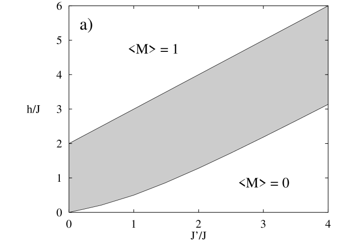
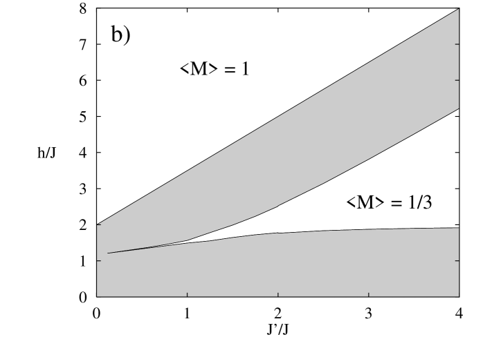
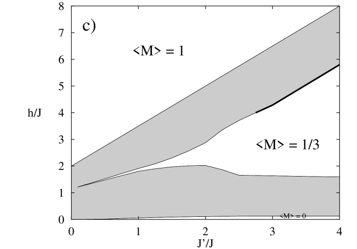
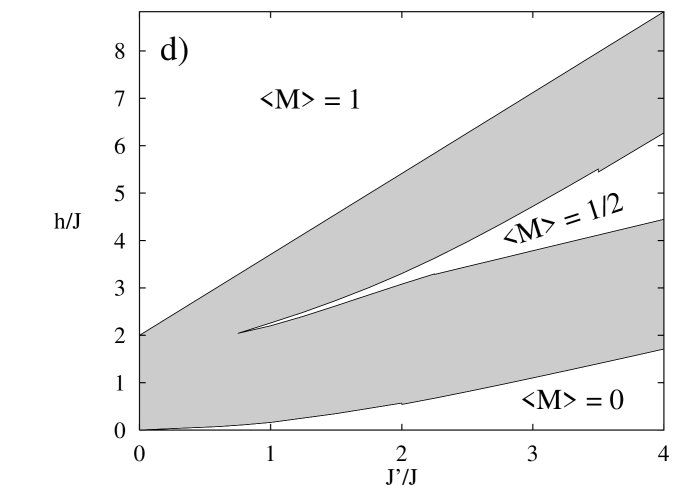
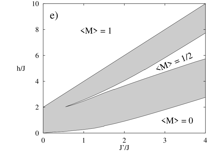
FIG. 6.: Schematic magnetic phase diagram at $\Delta=1$ for a) $N=2$, b) $N=3$ and OBC, c) $N=3$ and PBC, d) $N=4$ and OBC, e) $N=4$ and PBC. White regions in the $h$-${J^{\prime}}/J$ plane indicate gapped regions with a plateau in the magnetization curve while the shaded areas are massless and the magnetization $\langle M\rangle$ changes continuously if the applied field $h$ is varied.

Fig. 6b) shows a more interesting case, i.e. $N=3$ with OBC. The boundaries of the $\langle M\rangle=1/3$ plateau have been determined from the fourth order strong-coupling series (4.6) and (4.8) for ${J^{\prime}}/J\geq 2$. For $1\leq{J^{\prime}}/J\leq 2$ we obtained them from a Shanks extrapolation of the finite-size data in our earlier paper [15]. The remaining weak-coupling region is the most speculative part of the figure. We located the ending-point of the $\langle M\rangle=1/3$ plateau in the vicinity of the corresponding point on the magnetization curves of decoupled Heisenberg chains, as is suggested by the Abelian bosonization analysis if one assumes a similar behaviour for OBC and PBC (the bosonization analysis predicts for PBC that the $\langle M\rangle=1/3$ plateau disappears for small but non-zero ${J^{\prime}}/J$).

The analogous case with changed boundary conditions (i.e. $N=3$ and PBC) is shown in Fig. 6c). Here, no series expansions are possible due to extra degeneracies at strong coupling. The boundaries of the plateaux have therefore been determined in this case mainly on the basis of older numerical data [15]. We have used a Shanks extrapolation for $L=4$, $6$ and $8$ for ${J^{\prime}}/J\geq 2.75$ at the lower boundary of the $\langle M\rangle=1/3$ plateau and for ${J^{\prime}}/J=2.5$ at its upper boundary to estimate their location. For smaller couplings, the finite-size data is non-monotonic. The best we can do in the range $1\leq{J^{\prime}}/J\leq 2.5$ is to fit the $L=4$ and $8$ data to a form with $1/L$ corrections like (6.1,6.7). The ending point of the plateau is again placed on the basis of the weak-coupling analysis. It should be noted that the nature of the transition at the upper boundary of the $\langle M\rangle=1/3$ plateau changes qualitatively for ${J^{\prime}}/J\,\raise 2.0pt\hbox{$\mathop{>}\limits_{\raise 2.0pt\hbox{$\sim$}}$}\,2.75$ [15]. This strongly frustrated region is indicated by the bold line in Fig. 6c). It is possible that the transition becomes first order along this line. Note that the region in question is far outside the weak-coupling region, where we expect all transitions to be continuous.

Another interesting difference between Fig. 6b) and Fig. 6c) is that in the latter a tiny $\langle M\rangle=0$ plateau (i.e. a gap) opens. Its boundary has been estimated at intermediate couplings by fitting the $L=4$, $6$ and $8$ data [15] to the form (6.1). This yields slightly smaller values than those given in [57] in the cases where we overlap. However, we agree with [57] in the most important point, namely the existence of such a plateau. A numerical determination of its ending point is difficult, and the field-theoretical weak-coupling analysis is not yet conclusive either [53, 54] – the ending point may well be anywhere in the weak-coupling region $0\leq{J^{\prime}}\leq J$.

Finally, the magnetic phase diagrams for $N=4$ are given by Figs. 6d) and e) for OBC and PBC, respectively. To obtain them, we have performed further numerical computations. For the upper boundary of the $\langle M\rangle=1/2$ plateau we have numerical data for $L=4$, $6$ and $8$ such that we can apply a Shanks transform to it. For its lower boundary we have only $L=4$ and $6$ data and therefore we have to make an assumption on the finite-size corrections to extrapolate it (we assumed $1/L$ corrections, though this is not entirely satisfactory). In the strong-coupling region we used our series instead of numerical data. The series and numerical data are matched at ${J^{\prime}}/J=3.5$ or ${J^{\prime}}/J=2.5$ for the series corresponding to the upper boundary for OBC (4.24) or PBC (4.17), respectively. At the lower boundary of the $\langle M\rangle=1/2$ plateau we matched the series (4.23) and (4.15) to the numerical data at ${J^{\prime}}/J=2.25$ and ${J^{\prime}}/J=1.75$, respectively. Neither of the methods accessible to us is very accurate in the region where this plateau closes, but all three methods (numerical, series and Abelian bosonization) point to a location of the ending point in the region where ${J^{\prime}}$ and $J$ are of the same order.

The gaps for $N=4$ are taken from our series (4.20) for ${J^{\prime}}/J\geq 2$ for OBC and (4.11) for ${J^{\prime}}/J\geq 1.5$ for PBC. For OBC the accurate numerical data for the gap of [11] is used in the weak-coupling region. The corresponding line in Fig. 6e) is in comparison rather an educated guess which is inspired though by $L=4$ and $L=6$ numerical data. Regarding the series both for the gap and the boundaries of the $\langle M\rangle=1/2$ plateau, we observe a trend that those for PBC can be used for somewhat smaller values of ${J^{\prime}}/J$ than those for OBC. This is expected since the former are fourth order but the latter only second order.

Although Fig. 6 is for the particular choice $\Delta=1$ there is nothing particular about this case (at least for non-zero magnetizations), and one would obtain similar figures for other values of $\Delta$ as well. Further plateaux may open for $\Delta>1$. In particular, there should always be an $\langle M\rangle=0$ plateau in $N$ coupled XXZ-chains with $\Delta>1$, since each such chain is massive and this should be preserved at least for sufficiently weak coupling. In the Ising limit $\Delta\to\infty$ and for non-frustrating boundary conditions it is easy to see that this is accompanied by breaking of translational symmetry to a period $l=2$ in the groundstate. In the general case $\Delta>1$, such a period $l=2$ reconciles the appearance of a gap for both even and odd $N$ with (1.1).

The Abelian bosonization analysis predicts all the massless shaded regions in Fig. 6 to be $c=1$ theories (with the exception ${J^{\prime}}=0$ where one trivially has a $c=N$ theory). In these regions the exponents governing the asymptotics of the correlation functions depend continuously on the parameters. Predictions can be made, however, for the transitions at the boundaries between such massless phases and plateau regions. The opening of a plateau when varying ${J^{\prime}}$ is a transition of K-T type [45]. Like in the case of the transition at $\Delta=1$ in the XXZ-chain, this implies a very narrow plateau after the transition (c.f. (2.12)) which makes it difficult to observe numerically [15]. At the transition point the asymptotics of the correlation functions is governed by the exponents (3.19) while along the boundaries of the plateaux one has the universal exponents (3.20). It should be noted that an attempt to verify the latter exponents numerically or experimentally is likely to rather lead to the exponents characteristic for the transition point if one is sufficiently close to it.

The field-theoretical analysis also predicts the asymptotic behaviour of the magnetization in a massless phase but close to a plateau boundary to be given by the universal DN-PT behaviour [42, 43] (2.10). We have in fact numerically verified such a square-root behaviour close to saturation ($\langle M\rangle\to 1$) at some values of ${J^{\prime}}/J$ for $N=2$, $3$ and $4$ with both OBC and PBC. However, the example of the XXZ-chain shows (c.f. Fig. 2) that close to other plateau boundaries this universal behaviour may be restricted to a tiny region and its observation could be very difficult. In experimental situations, it will be further obscured by thermal fluctuations and other effects such as disorder (see e.g. [17]). This explains why rather accurate experiments on $N=2$ leg spin-ladder materials [16, 63] show no evidence of a square-root behaviour for $\langle M\rangle\to 0$.

Quite surprisingly, massless excitations (though non-magnetic ones) also arise in plateau regions. This can be seen from (5.3) which for $\langle M\rangle=1/N$ is just an XY-chain and therefore massless. This yields massless excitations in the limit ${J^{\prime}}\to\infty$ in Fig. 6c), or more generally in the strong-coupling limit on the $\langle M\rangle=1/N$ plateau for $N$ odd and PBC. Whether $J/{J^{\prime}}=0$ is just a critical point or if massless non-magnetic excitations also arise at finite ${J^{\prime}}$ remains to be investigated.

VIII Discussion and Conclusion

In this paper we have investigated the conditions under which plateaux appear in $N$-leg spin ladders as well as the universality classes of the transitions at the boundaries of such plateaux. Certain small plateaux may have slipped our attention. For example, there could be a narrow $\langle M\rangle=2/3$ plateau for $N=3$ and PBC at intermediate or strong coupling ${J^{\prime}}$ which would be accompanied by spontaneous breaking of translational symmetry to a period $l=2$. If this should turn out to be the case, it would have to be added to Fig. 6c). However, our main point is the presence of such plateaux, not the absence of particular ones.

We also confirmed the conclusion of [57] that in the case $N=3$ frustration induces a zero-field gap at least for sufficiently strong coupling. It may be even more intriguing that, according to our strong-coupling data, this gap seems to survive the $N\to\infty$ limit for an odd number $N$ of cylindrically coupled chains. This shows that it is necessary to specify at least boundary conditions along the rungs in the generalization of the Haldane conjecture to spin ladders. The peculiar behaviour of a cylindrical configuration may be interpreted as follows: Strongly frustrating boundary conditions force a one-dimensional domain wall into the two-dimensional system corresponding to $N=\infty$. The $N\to\infty$ limit of the one-dimensional Hamiltonian (5.3) is just the effective Hamiltonian for the low-energy excitations of this domain wall. As a consequence, there cannot be any long-range order which is typical for the two-dimensional Heisenberg model, and there is no reason why the low-energy spectrum should not be gapped as it apparently is.

Similar surprises cannot be completely ruled out in the weak-coupling region for $N$ even and $\langle M\rangle=0$. The zero-field case is difficult to control since there is an additional relevant interaction between the massive degrees of freedom and the possibly massless ones (the coefficient of $\lambda_{2}$ in (3.7)). In general, this gives rise to non-perturbative renormalization. In the isotropic case $\Delta=1$ one can use the $SU(2)$ symmetry [52] to infer the renormalized radius of compactification of the remaining massless field. This then leads to the generalized Haldane conjecture in the framework of Abelian bosonization. For $\Delta>1$ a gap is always expected in the weak-coupling regime since already the decoupled chains are massive. The situation is far less clear for anisotropies $\Delta<1$ since then it is not known how to control the renormalization group flow. An investigation of this region by other non-perturbative methods would be interesting. It may also be desirable to perform further checks of the absence of an extended massless phase in the $SU(2)$ symmetric situation for even $N\geq 6$.

Beyond a more detailed understanding of the $N$-leg spin-ladder model (3.1) treated here, a similar investigation of other models could be interesting. One natural step would be to include charge degrees of freedom, and see if interesting effects arise from the interplay of a magnetic field with transport properties.

Last but not least, it would be desirable to have an experimental verification of our predictions. We are confident that this is possible in principle and hope that it will in fact be carried out.

Acknowledgments: We would like to thank F.C. Alcaraz, G. Albertini, F.H.L. Eßler, T. Giamarchi, M. Oshikawa, K. Totsuka and B. Wehefritz for helpful discussions concerning in particular a single XXZ-chain. D.C.C. is grateful to CONICET and Fundación Antorchas for financial support. We are indebted to the Max-Planck-Institut für Mathematik Bonn-Beuel where the more complicated numerical computations have been performed.

REFERENCES

- [1] E. Dagotto, T.M. Rice, Science 271, 618 (1996); T.M. Rice, Z. Phys. B103, 165 (1997).
- [2] M. Azuma, Z. Hiroi, M. Takano, K. Ishida, Y. Kitaoka, Phys. Rev. Lett. 73, 3463 (1994).
- [3] E. Dagotto, J. Riera, D.J. Scalapino, Phys. Rev. B45, 5744 (1992); T. Barnes, E. Dagotto, J. Riera, E.J. Swanson, Phys. Rev. B47, 3196 (1993).
- [4] F.D.M. Haldane, Phys. Rev. Lett. 50, 1153 (1983).
- [5] T. Ziman, H.J. Schulz, Phys. Rev. Lett. 59, 140 (1987); M. Takahashi, Phys. Rev. Lett. 62, 2313 (1989); O. Golinelli, T. Jolicoeur, R. Lacaze, Phys. Rev. B50, 3037 (1994); K. Hallberg, X.Q.G. Wang, P. Horsch, A. Moreo, Phys. Rev. Lett. 76, 4955 (1996).
- [6] D.C. Cabra, P. Pujol, C. von Reichenbach, Phys. Rev. B58, 65 (1998).
- [7] G. Sierra, p. 136 in Strongly Correlated Magnetic and Superconducting Systems, eds. G. Sierra, M.A. Martín-Delgado, Lecture Notes in Physics 478 (Springer, Berlin, 1997) [cond-mat/9610057].
- [8] M. Reigrotzki, H. Tsunetsugu, T.M. Rice, J. Phys.: Condensed Matter 6, 9235 (1994).
- [9] S.R. White, R.M. Noack, D.J. Scalapino, Phys. Rev. Lett. 73, 886 (1994).
- [10] B. Frischmuth, B. Ammon, M. Troyer, Phys. Rev. B54, R3714 (1996).
- [11] M. Greven, R.J. Birgeneau, U.-J. Wiese, Phys. Rev. Lett. 77, 1865 (1996).
- [12] M. Oshikawa, M. Yamanaka, I. Affleck, Phys. Rev. Lett. 78, 1984 (1997).
- [13] K. Totsuka, Phys. Lett. A228, 103 (1997).
- [14] K. Totsuka, Phys. Rev. B57, 3454 (1998).
- [15] D.C. Cabra, A. Honecker, P. Pujol, Phys. Rev. Lett. 79, 5126 (1997).
- [16] G. Chaboussant, P.A. Crowell, L.P. Lévy, O. Piovesana, A. Madouri, D. Mailly, Phys. Rev. B55, 3046 (1997).
- [17] C.A. Hayward, D. Poilblanc, L.P. Lévy, Phys. Rev. B54, R12649 (1996).
- [18] Z. Weihong, R.R.P. Singh, J. Oitmaa, Phys. Rev. B55, 8052 (1997).
- [19] R. Chitra, T. Giamarchi, Phys. Rev. B55, 5816 (1997).
- [20] J.B. Parkinson, J.C. Bonner, Phys. Rev. B32, 4703 (1985).
- [21] E. Lieb, T. Schultz, D. Mattis, Ann. Phys. 16, 407 (1961).
- [22] I. Affleck, Phys. Rev. B37, 5186 (1988).
- [23] A.G. Rojo, Phys. Rev. B53, 9172 (1996).
- [24] A. Honecker, M. Kaulke, K.D. Schotte, in preparation.
- [25] F.D.M. Haldane, Phys. Rev. Lett. 45, 1358 (1980).
- [26] F. Woynarovich, H.-P. Eckle, T.T. Truong, J. Phys. A: Math. Gen. 22, 4027 (1989).
- [27] I. Affleck, p. 563 in Fields, Strings and Critical Phenomena, Les Houches, Session XLIX, eds. E. Brézin, J. Zinn-Justin (North-Holland, Amsterdam, 1988).
- [28] N.M. Bogoliubov, A.G. Izergin, V.E. Korepin, Nucl. Phys. B275, 687 (1986).
- [29] V.E. Korepin, N.M. Bogoliubov, A.G. Izergin, Quantum Inverse Scattering Method and Correlation Functions, Cambridge University Press, Cambridge (1993).
- [30] S. Qin, M. Fabrizio, L. Yu, M. Oshikawa, I. Affleck, Phys. Rev. B56, 9766 (1997).
- [31] URL http://www.he.sissa.it/~honecker/roc.html (backup under URL http://thew02.physik.uni-bonn.de/~honecker/roc.html).
- [32] F.C. Alcaraz, A.L. Malvezzi, J. Phys. A: Math. Gen. 28, 1521 (1995).
- [33] J.D. Noh, D. Kim, Phys. Rev. E53, 3225 (1996).
- [34] O. Babelon, H.J. de Vega, C.M. Viallet, Nucl. Phys. B220, 13 (1983).
- [35] Y.A. Izyumov, Y.N. Skryabin, Statistical Mechanics of Magnetically Ordered Systems, Consultants Bureau, New York (1988), section 17.
- [36] F.C. Alcaraz, private communication.
- [37] J. des Cloizeaux, M. Gaudin, J. Math. Phys. 7, 1384 (1966).
- [38] L.D. Faddeev, L.A. Takhtajan, Phys. Lett. A85, 375 (1981).
- [39] G. Gómez-Santos, Phys. Rev. B41, 6788 (1990).
- [40] T.M. Rice, S. Haas, M. Sigrist, F.-C. Zhang, Phys. Rev. B56, 14655 (1997).
- [41] J.D. Johnson, B.M. McCoy, Phys. Rev. A6, 1613 (1972).
- [42] G.I. Dzhaparidze, A.A. Nersesyan, JETP Lett. 27, 334 (1978).
- [43] V.L. Pokrovsky, A.L. Talapov, Phys. Rev. Lett. 42, 65 (1979).
- [44] R.P. Hodgson, J.B. Parkinson, J. Phys. C: Solid State Phys. 18, 6385 (1985).
- [45] J.M. Kosterlitz, D.J. Thouless, J. Phys. C: Solid State Phys. 6, 1181 (1973).
- [46] A. Luther, Phys. Rev. B14, 2153 (1976).
- [47] D.J. Amit, Y.Y. Goldschmidt, G. Grinstein, J. Phys. A: Math. Gen. 13, 585 (1980).
- [48] M.P.M. den Nijs, Phys. Rev. B23, 6111 (1981).
- [49] J.M. Kosterlitz, J. Phys. C: Solid State Phys. 7, 1046 (1974).
- [50] H.J. Schulz, Phys. Rev. B22, 5274 (1980).
- [51] H.J. Schulz, Phys. Rev. B34, 6372 (1986).
- [52] H.J. Schulz, p. 81 in Correlated Fermions and Transport in Mesoscopic Systems, eds. T. Martin, G. Montambaux, J. Tran Thanh Van (Editions Frontières, Gif–sur–Yvette, 1996) [cond-mat/9605075].
- [53] E. Arrigoni, Phys. Lett. A215, 91 (1996).
- [54] M. Suzuki, K. Totsuka, J. Phys. A: Math. Gen. 29, 3559 (1996).
- [55] A. Honecker, J. Stat. Phys. 82, 687 (1996).
- [56] Z. Weihong, V. Kotov, J. Oitmaa, Phys. Rev. B57, 11439 (1998).
- [57] K. Kawano, M. Takahashi, J. Phys. Soc. Jpn. 66, 4001 (1997).
- [58] P.P. Kulish, E.K. Sklyanin, p. 61 in Integrable Quantum Field Theories, eds. J. Hietarinta, C. Montonen, Lecture Notes in Physics 151 (Springer, Berlin, 1982).
- [59] M. Henkel, G.M. Schütz, J. Phys. A: Math. Gen. 21, 2617 (1988).
- [60] S.P. Strong, A.J. Millis, Phys. Rev. B50, 9911 (1994).
- [61] K. Totsuka, M. Suzuki, J. Phys.: Condensed Matter 7, 6079 (1995).
- [62] D.G. Shelton, A.A. Nersesyan, A.M. Tsvelik, Phys. Rev. B53, 8521 (1996).
- [63] W. Shiramura, K. Takatsu, H. Tanaka, K. Kamishima, M. Takahashi, H. Mitamura, T. Goto, J. Phys. Soc. Jpn. 66, 1900 (1997).