Asymptotic power law of moments in a random multiplicative process
with weak additive noise

Abstract

It is well known that a random multiplicative process with weak additive noise generates a power-law probability distribution. It has recently been recognized that this process exhibits another type of power law: the moment of the stochastic variable scales as a function of the additive noise strength. We clarify the mechanism for this power-law behavior of moments by treating a simple Langevin-type model both approximately and exactly, and argue this mechanism is universal. We also discuss the relevance of our findings to noisy on-off intermittency and to singular spatio-temporal chaos recently observed in systems of non-locally coupled elements.

I Introduction

Power laws are observed in a wide variety of natural phenomena and mathematical models. Some examples are the critical behavior near second order phase transitions, Kolmogorov’s law of fully developed turbulence, size distribution of avalanches in models of self-organized criticality, Gutenberg-Richter’s law of earthquakes, distribution of price fluctuations in economic activities, and Zipf’s law in linguistics. Clarifying the mechanisms for the emergence of these power laws has long been a subject of many challenges.

The random multiplicative process (RMP) is a well-known mechanism leading to power-law behavior. It is a stochastic process where the stochastic variable is driven by a multiplicative noise. It has been extensively used as a model for a variety of systems such as on-off intermittency [1, 2, 3, 4, 5, 6], lasers [7], economic activity [8, 9], variation of biological populations in fluctuating environment [10], and passive scalar field advected by fluid [11].

In real systems, the stochastic variable may often be driven not only by the multiplicative noise, but also by some weak additive noise. This weak additive noise becomes important when the amplitude of the stochastic variable $x$ takes small values, and introduces an effective lower bound of $x$. Actually, this lower bound may be crucial, because it guarantees the existence of a stationary probability distribution function (PDF). Furthermore, the PDF here has a power-law form over a wide range of $x$ [1, 3, 5, 8, 9, 11, 13].

For example, Venkataramani et al. [5] introduced a Langevin equation with multiplicative and additive noise terms as a model for noisy on-off intermittency. They obtained a stationary PDF with a power-law tail. The same form of Langevin equation was treated by Takayasu et al. [9] as a model for economic activity, and they also showed that the PDF obeys a power law. A similar model was introduced by Levy et al. [8]: it describes a discrete stochastic process driven by a multiplicative noise. They introduced a lower bound to the stochastic variable explicitly, and showed again that the PDF obeys a power law. Venkataramani et al. and Takayasu et al. treated the additive noise explicitly, while the lower bound introduced by Levy et al. plays a role similar to the additive noise. In this paper, we are concerned with this type of stochastic processes.

Recently, another type of asymptotic power law was found in the above type of stochastic processes. In previous papers [12, 13], we introduced a stochastic process in order to explain the power law displayed by the spatial correlation function $C(r)$, i.e., $C(r)\simeq C_{0}-C_{1}r^{\alpha}$ for small enough $r$, observed in the spatio-temporal chaotic regime of systems with non-locally coupled elements. Our explanation was based on a RMP with weak additive noise such as described above. Note, however, that the power-law correlation here is not a direct result of the power-law tail of the PDF itself, but it is a result of the asymptotic power law of moments $<x^{q}>$ of the stochastic variable $x$ as a function of the strength $s$ of the additive noise, i.e., $<x^{q}>\simeq G_{0}+G_{1}s^{H(q)}$. This gives another mechanism leading to power-law behavior in such stochastic processes.

The goal of this paper is to clarify this mechanism for the emergence of the power law of moments with respect to the strength of the additive noise. We achieve this by using a simple Langevin-type model, and argue that the mechanism proposed is a universal one in generating various power laws.

The outline of this paper is as follows: In Sec. II we introduce the model to be studied, and display its typical behavior. In Sec. III we treat the model approximately in order to outline the mechanism for the emergence of the power law of moments, and then exactly in Sec. IV. In Sec. V we discuss the robustness of the power law with regard to boundary conditions and nature of the noise. We also show some results obtained by numerical calculations with colored noises. In Sec. VI we discuss an application of our theory to noisy on-off intermittency. As an example, we show a result obtained by a numerical calculation of coupled chaotic elements. Furthermore, we discuss the relation of the power law of moments to the power-law spatial correlations observed in systems of non-locally coupled chaotic elements. We summarize our results in Sec. VII.

II Analytical model

A Langevin equation

As a model for a RMP with weak additive noise, we employ a Langevin equation

$$\frac{dx(t)}{dt}=\lambda(t)x(t)+\eta(t),$$ (1)

where $x(t)$ is a stochastic variable, $\lambda(t)$ a multiplicative noise, and $\eta(t)$ an additive noise. We assume both $\lambda(t)$ and $\eta(t)$ to be Gaussian-white, and their average and variance to be given by

$$\begin{array}[]{c}<\lambda(t)>=\lambda_{0},\ <\left[\lambda(t)-\lambda_{0}\right]\left[\lambda(t^{\prime})-\lambda_{0}\right]>=2D_{\lambda}\delta(t-t^{\prime}),\\ \\ <\eta(t)>=0,\ <\eta(t)\ \eta(t^{\prime})>=2D_{\eta}\delta(t-t^{\prime}).\end{array}$$ (2)

We further assume $D_{\eta}\ll D_{\lambda}$, namely, the additive noise is sufficiently weaker than the multiplicative noise.

This simple Langevin equation (1) has been widely used in many studies of various systems [5, 7, 9, 11]. The physical meaning of $x(t)$, $\lambda(t)$, and $\eta(t)$ may be different depending on the specific system under consideration. For example, in the case of lasers, $x(t)$ gives the number of photons, $\lambda(t)$ its fluctuating amplification rate, and $\eta(t)$ the noise due to random spontaneous emissions of atoms. When we are working with noisy on-off intermittency, $x(t)$ gives the measure of a distance from the invariant manifold, $\lambda(t)$ the instantaneous vertical Lyapunov exponent, and $\eta(t)$ the noise due to a parameter mismatch or some other cause. In the context of economic models, $x(t)$ represents the wealth, $\lambda(t)$ the rate of change of the wealth, and $\eta(t)$ some external noise of various sources.

B Boundary conditions

In order to obtain a statistically stationary state from the Langevin equation (1), we generally need upper and lower bounds of $x$. In our model, the weak additive noise may act as an effective lower bound.

(a) Lower bound

Without the additive noise, $x(t)$ tends to $0$ when the average expansion rate $\lambda_{0}$ is negative. The additive noise introduces an effective lower bound of $x(t)$, which keeps $x(t)$ away from the zero value even if $\lambda_{0}<0$. In this paper, we treat the additive noise explicitly, while in some other studies it is replaced by a reflective wall (infinitely high barrier) placed at some small $x$.

(b) Upper bound

To be realistic, when $x(t)$ takes too large values, it should be saturated by some effect such as nonlinearity. We simply introduce this effect as boundary conditions, specifically reflective walls at $x=\pm 1$.

With these upper and lower bounds provided by an additive noise and reflective walls, the Langevin equation (1) admits a statistically stationary state. In Fig. 1, we show a typical time evolution of $x(t)$ governed by the Langevin equation (1) for slightly negative $\lambda_{0}$, where the reflective walls are placed at $x=\pm 1$. In spite of the negative average expansion rate $\lambda_{0}$, $x(t)$ does not simply decay but exhibits intermittent bursts. The generation of bursts may be interpreted as follows. Due to the weak additive noise, $x(t)$ may generally have small but finite values. If positive $\lambda(t)$ happens to persist over some period, $x(t)$ will be amplified exponentially and attain large values, which is nothing but bursts. Of course, $x(t)$ may eventually decay to the noise level because of negative $\lambda_{0}$. The chance of bursts will increase with the additive noise strength. Why this leads to a power-law dependence of moments of $x(t)$ on the additive noise strength can be understood from the argument below.

The intermittency described above has the same statistical nature as the noisy on-off intermittency. Actually, one may consider the noisy on-off intermittency as a stochastic process of the type described above.

FIG. 1.: Typical time evolution of the amplitude $x(t)$ of the Langevin equation (1) for $\lambda_{0}=-0.5$, $D_{\lambda}=0.5$, $D_{\eta}=0.00005$.

III Approximate treatment

In order to give an outline of the mechanism underlying the emergence of the power law of moments, we first treat the Langevin equation (1) approximately.

A Fokker-Planck equation

We introduce a characteristic amplitude

$$s=\sqrt{\frac{D_{\eta}}{D_{\lambda}}}\ \ \ (0<s<1)$$ (3)

which results from the balance between the fluctuation due to the multiplicative noise $<(\lambda x)^{2}>$$\sim D_{\lambda}x^{2}$ and the fluctuation due to the additive noise $<\eta^{2}>$$\sim D_{\eta}$. We divide the range of $x$ into two parts, $0<|x|<s$ and $s<|x|<1$, and ignore in each region one of the noise sources which is less dominant there. Since the system is statistically symmetric with respect to the transformation $x\rightarrow-x$, we consider only the absolute value $|x|$ hereafter.

(a) $s<|x|<1$

In this region, we ignore the effect of the additive noise and consider a Langevin equation

$$\frac{dx(t)}{dt}=\lambda(t)x(t).$$ (4)

By introducing a new variable $y(t)=\log|x(t)|$, Eq. (4) is rewritten as

$$\frac{dy(t)}{dt}=\lambda(t),$$ (5)

which gives a diffusion process with mean drift.

Let $P_{1}(x,t)$ denote the PDF of $x(t)$ and ${\bar{P}_{1}}(y,t)$ the corresponding PDF of $y(t)$. The Fokker-Planck equation corresponding to Eq. (4) takes the form

$$\frac{\partial}{\partial t}{\bar{P}_{1}}(y,t)=-\frac{\partial}{\partial y}j_{1}(y,t),$$ (6)

where the flux $j_{1}(y,t)$ is given by

$$j_{1}(y,t)=\lambda_{0}{\bar{P}_{1}}(y,t)-D_{\lambda}\frac{\partial}{\partial y}{\bar{P}_{1}}(y,t).$$ (7)

Setting reflective walls at $x=\pm 1$ is equivalent to assuming a no-flux boundary condition for $j_{1}$ at $y=0$, i.e., $j_{1}(y=0,t)=0$.

(b) $0<|x|<s$

In this region, we ignore the effect of the multiplicative noise, and this leads to a Langevin equation

$$\frac{dx(t)}{dt}=\eta(t).$$ (8)

Let $P_{2}(x,t)$ be the PDF of $x(t)$. $P_{2}(x,t)$ obeys the Fokker-Planck equation

$$\frac{\partial}{\partial t}P_{2}(x,t)=-\frac{\partial}{\partial x}j_{2}(x,t),$$ (9)

where the flux $j_{2}(x,t)$ is now defined by

$$j_{2}(x,t)=-D_{\eta}\frac{\partial}{\partial x}P_{2}(x,t).$$ (10)

The boundary conditions to be imposed here are the continuity of $P_{1}$ and $P_{2}$, and also $j_{1}$ and $j_{2}$, each at $|x|=s\ (y=\log s)$.

B Stationary PDF with a power-law tail

We calculate here the stationary solution of the Fokker-Planck equation.

(a) $s<|x|<1$

Stationarity condition ${\partial{\bar{P}_{1}}}/{\partial t}=0$ gives ${\partial j_{1}}/{\partial y}=0$, i.e., $j_{1}(y)\equiv const.$, and the no-flux boundary condition $j_{1}(y=0)=0$ gives $j_{1}(y)\equiv 0$. Therefore, the stationary solution ${\bar{P}_{1}}(y)$ satisfies

$$0=\lambda_{0}{\bar{P}_{1}}(y)-D_{\lambda}\frac{\partial}{\partial y}{\bar{P}_{1}}(y).$$ (11)

This can be solved as

$${\bar{P}_{1}}(y)=C\exp\left(\frac{\lambda_{0}}{D_{\lambda}}y\right),$$ (12)

where $C$ is a normalization constant. In terms of the original variable $x$, we obtain

$$P_{1}(x) = {\bar{P}_{1}}(y)\frac{dy}{dx}$$ (13)

$$= C\frac{1}{|x|}\exp\left(\frac{\lambda_{0}}{D_{\lambda}}\log(|x|)\right)$$ (14)

$$= C|x|^{\frac{\lambda_{0}}{D_{\lambda}}-1}.$$ (15)

Thus, the PDF obeys a power law in this region. The exponent of this power law is determined by the ratio of $\lambda_{0}$ to $D_{\lambda}$, i.e., by the basic statistical characteristics of the multiplier $\lambda(t)$, and does not depend on the nature of the additive noise. We denote this ratio as $\beta$ hereafter:

$$\beta=\frac{\lambda_{0}}{D_{\lambda}}.$$ (16)

(b) $0<|x|<s$

A general form of the stationary solution is given by $P_{2}(x)=Ax+B$, where $A$ and $B$ are constants. Continuity of the flux and the PDF at $|x|=s$, i.e., $j_{2}(s)=j_{1}(s)\equiv 0$ and $P_{2}(s)=P_{1}(s)$ gives $A=0$ and $B=P_{1}(s)$. Therefore, $P_{2}(x)$ takes a constant value:

$$P_{2}(x)\equiv P_{1}(s)=Cs^{\frac{\lambda_{0}}{D_{\lambda}}-1}.$$ (17)

Finally, the approximate stationary PDF is obtained as

$$P(x)=\left\{\begin{array}[]{cc}Cs^{\beta-1}&(0<|x|<s)\\ \\ Cx^{\beta-1}&(s<|x|<1)\\ \\ 0&(|x|>1)\end{array}\right..$$ (18)

The normalization constant $C$ is determined from

$$\int_{-1}^{1}P(x)dx=2\int_{0}^{1}P(x)dx=1,$$ (19)

and calculated as

$$C = \left[2\left(\int_{0}^{s}s^{\beta-1}dx+\int_{s}^{1}x^{\beta-1}dx\right)\right]^{-1}$$ (20)

$$= \left[2\left(s^{\beta}+\frac{1-s^{\beta}}{\beta}\right)\right]^{-1}.$$ (21)

Thus, the PDF consists of three parts, i.e., a constant part near the origin where $x(t)$ is dominated by a normal diffusion process, a power-law tail where $x(t)$ is dominated by a RMP, and a vanishing part. The boundary between the constant part and the power-law tail is located at $|x|=s$, which is proportional to the additive noise strength $\sqrt{D_{\eta}}$. We show this approximate PDF (18) in Fig. 2.

FIG. 2.: PDFs $P(x)$ vs. $x$, where the approximate and exact curves are compared. The parameters are the same as in Fig. 1.

C Moments

The $q$-th moment $<x^{q}>$ of $|x|$ in this stationary state (18) is calculated as

$$<x^{q}> = \int_{-1}^{1}|x|^{q}P(x)dx=2\int_{0}^{1}x^{q}P(x)dx$$ (22)

$$= 2C\left(\int_{0}^{s}x^{q}s^{\beta-1}dx+\int_{s}^{1}x^{q}x^{\beta-1}dx\right)$$ (23)

$$= \frac{\beta}{\beta+q}\frac{1+(\frac{\beta+q}{1+q}-1)s^{\beta+q}}{1+(\beta-1)s^{\beta}}.$$ (24)

We can write the above in the form

$$<x^{q}>=c_{q}\frac{1+a_{q}s^{\beta+q}}{1+a_{0}s^{\beta}},$$ (25)

where $c_{q}$ and $a_{q}$ are given by

$$c_{q}=\frac{\beta}{\beta+q},\ \ \ a_{q}=\frac{\beta+q}{1+q}-1.$$ (26)

Note that the exponent $\beta$ of the PDF now appears as the power of $s$. As we explain below, the form of Eq. (25) is all we need for the emergence of the asymptotic power law of moments.

D Asymptotic forms of the moments

We investigate the asymptotic forms of the moment $<x^{q}>$ in the limit of small additive noise $s$. We consider only the practically interesting case of positive $q$.

(a) $\beta>0$

By expanding the denominator of $<x^{q}>$ and taking the lowest order in $s$, we obtain

$$<x^{q}>\simeq c_{q}\left(1-a_{0}s^{\beta}\right).$$ (27)

(b) $\beta<0$

Ignoring $1$ in the denominator of $<x^{q}>$, we obtain

$$<x^{q}>\simeq\frac{c_{q}}{a_{0}}\left(s^{|\beta|}+a_{q}s^{q}\right).$$ (28)

Which of $|\beta|$ and $q$ is smaller determines which of the two terms on the right-hand side of Eq. (28) dominates. We thus obtain

$$<x^{q}>\simeq\left\{\begin{array}[]{ll}\displaystyle{\frac{c_{q}}{a_{0}}s^{|\beta|}}&(|\beta|<q)\\ \\ \displaystyle{\frac{c_{q}a_{q}}{a_{0}}s^{q}}&(|\beta|>q)\end{array}\right..$$ (29)

These results show that the moment $<x^{q}>$ approaches a simple power-law form as a function of the position $s$ of the boundary, or the strength $\sqrt{D_{\eta}}$ of the additive noise:

$$<x^{q}>\simeq G_{0}+G_{1}s^{H(q)},$$ (30)

where $G_{0}$ and $G_{1}$ are constants. $G_{0}$ vanishes when $\beta<0$ ($\lambda_{0}<0$), while it takes a finite value when $\beta>0$ ($\lambda_{0}>0$). Thus, we have obtained the power law of moments.

E Exponents

The exponent $H(q)$ of the moment $<x^{q}>$ is determined by $\beta$, namely, the ratio of $\lambda_{0}$ to $D_{\lambda}$. From Eqs. (27) and (29), $H(q)$ varies with $q$ as follows:

(a) $\beta<0$

$$H(q)=\left\{\begin{array}[]{cc}q&(0<q<|\beta|)\\ \\ |\beta|&(|\beta|<q)\end{array}\right.,$$ (31)

(b) $\beta>0$

$$H(q)=\beta.$$ (32)

We notice that $H(q)=q$ when $0<q<|\beta|$, but $H(q)=|\beta|$ when $|\beta|<q$ or $\beta>0$ without dependence on $q$.

F Other asymptotic regimes

When $\beta\simeq 0$ or $|\beta|\simeq q$, there exist other asymptotic regimes where the asymptotic form of the moment in the $s\rightarrow 0$ limit is not a power law.

(a) $\beta\simeq 0$

Consider a parameter region where $\beta\simeq 0$ and $|\beta\log s|\ll 1$. The denominator of $<x^{q}>$ can be expanded as

$$1+a_{0}s^{\beta} = 1+a_{0}\exp(\beta\log s)$$ (33)

$$= 1+a_{0}+a_{0}\beta\log s+{\it O}(|\beta\log s|^{2}).$$ (34)

Using $a_{0}=\beta-1$ and $|\log s|\gg 1$, the $a_{0}\beta\log s$ term is found to be dominant and we obtain

$$<x^{q}>\simeq\frac{c_{q}}{|a_{0}\beta\log s|}.$$ (35)

Thus $<x^{q}>$ diverges logarithmically as $1/|\log s|$.

(b) $|\beta|\simeq q$

Consider a parameter region where $\beta<0$ and $|\beta|\simeq q$. We further assume $|(q-|\beta|)\log s|\ll 1$. $<x^{q}>$ is then given by

$$<x^{q}>\simeq\frac{c_{q}}{a_{0}}\left(s^{|\beta|}+a_{q}s^{q}\right)=\frac{c_{q}}{a_{0}}s^{|\beta|}\left(1+a_{q}s^{q-|\beta|}\right).$$ (36)

Expanding the right-hand side, we obtain

$$1+a_{q}s^{q-|\beta|} = 1+a_{q}\exp\left((q-|\beta|)\log s\right)$$ (37)

$$= 1+a_{q}+a_{q}(q-|\beta|)\log s$$ (39)

$$\ \ \ \ \ \ \ \ \ +{\it O}(|(q-|\beta|)\log s|^{2}).$$

By using $a_{q}=\frac{\beta+q}{1+q}-1$ and $|\log s|\gg 1$, the $a_{q}(q-|\beta|)\log s$ term is found to be dominant, and we obtain

$$<x^{q}>\simeq\frac{c_{q}a_{q}}{a_{0}}|(q-|\beta|)s^{|\beta|}\log s|.$$ (40)

Thus $<x^{q}>$ diverges as $|s^{|\beta|}\log s|$.

IV Exact treatment

Next, we treat the effect of the additive noise without approximation. The argument below is in parallel with the previous one, and their results agree qualitatively, giving the same values of the exponents. How to calculate the PDF follows the argument by Venkataramani et al. [5].

A Fokker-Planck equation

The Fokker-Planck equation corresponding to the Langevin equation (1) is given by

$$\frac{\partial}{\partial t}P(x,t)=-\frac{\partial}{\partial x}j(x,t),$$ (41)

where $P(x,t)$ is the PDF of $x(t)$, and the flux $j(x,t)$ takes the form

$$j(x,t)=(\lambda_{0}+D_{\lambda})xP(x,t)-\frac{\partial}{\partial x}[(D_{\lambda}x^{2}+D_{\eta})P(x,t)].$$ (42)

Reflective walls at $x=\pm 1$ are equivalent to imposing no-flux boundary conditions at $x=\pm 1$, i.e.,

$$j(x=\pm 1,t)=0.$$ (43)

B Stationary PDF with a power-law tail

We calculate the stationary solution $P(x)$ of the Fokker-Planck equation (41). Stationarity condition ${\partial P(x,t)}/{\partial t}=0$ gives ${\partial j(x,t)}/{\partial x}=0$, i.e., $j(x)\equiv const.$, and no-flux boundary conditions $j(x=\pm 1)=0$ give $j(x)\equiv 0$. Therefore, $P(x)$ obeys

$$(\lambda_{0}+D_{\lambda})xP(x)-\frac{\partial}{\partial x}[(D_{\lambda}x^{2}+D_{\eta})P(x)]=0.$$ (44)

Solving this, we obtain

$$P(x)=C(D_{\lambda}x^{2}+D_{\eta})^{\frac{\lambda_{0}}{2D_{\lambda}}-\frac{1}{2}}$$ (45)

as the stationary PDF, where $C$ is a normalization constant to be determined from

$$\int_{-1}^{1}P(x)dx=2\int_{0}^{1}P(x)dx=1.$$ (46)

If we use the integral formula

$${\int_{0}^{1}(1+cx^{2})^{a}dx={{}_{2}F_{1}}(-a,\frac{1}{2},\frac{3}{2};-c)},$$ (47)

where ${{}_{2}F_{1}}(a,b,c;z)$ is the hypergeometric function, $C$ can be expressed as

$$C=\left[2D_{\eta}^{\frac{\lambda_{0}}{2D_{\lambda}}-\frac{1}{2}}\ {{}_{2}F_{1}}(-\frac{\lambda_{0}}{2D_{\lambda}}+\frac{1}{2},\frac{1}{2},\frac{3}{2};-\frac{D_{\lambda}}{D_{\eta}})\right]^{-1}.$$ (48)

We define $\beta$ as the ratio of the average expansion rate $\lambda_{0}$ to its fluctuation $D_{\lambda}$ as in the previous calculation, and $\alpha$ as the exponent of $P(x)$, i.e.,

$$\beta=\frac{\lambda_{0}}{D_{\lambda}},\ \ \ \alpha=\frac{\beta-1}{2}=\frac{\lambda_{0}}{2D_{\lambda}}-\frac{1}{2}.$$ (49)

Further, we define $s$ as the ratio of the strength $\sqrt{D_{\eta}}$ of the additive noise to the strength $\sqrt{D_{\lambda}}$ of the multiplicative noise:

$$s=\sqrt{\frac{D_{\eta}}{D_{\lambda}}}.$$ (50)

Finally, the stationary PDF is expressed as

$$P(x)=\left\{\begin{array}[]{cc}\displaystyle{\frac{(1+\frac{x^{2}}{s^{2}})^{\alpha}}{2{{}_{2}F_{1}}(-\alpha,\frac{1}{2},\frac{3}{2};-\frac{1}{s^{2}})}}&(|x|<1)\\ \\ 0&(|x|>1)\end{array}\right..$$ (51)

This stationary PDF approaches a constant as $x\rightarrow 0$, and when $s^{2}\ll 1$, namely, when the additive noise is sufficiently weaker than the multiplicative noise, the PDF approaches a power law as $x\rightarrow\pm 1$:

$$P(x)\sim\left\{\begin{array}[]{ll}const.&(x\rightarrow 0)\\ \\ |x|^{2\alpha}&(x\rightarrow\pm 1)\end{array}\right..$$ (52)

The exponent of this power law is given by

$$2\alpha=\beta-1=\frac{\lambda_{0}}{D_{\lambda}}-1.$$ (53)

Thus, we obtain qualitatively the same PDF as the previous approximate result (18), in particular, a power law with the same exponent. The crossover point between the constant region and the power-law region of the PDF is found from the balance of the two terms in the numerator of $P(x)$:

$$1\simeq\frac{x^{2}}{s^{2}}.$$ (54)

The crossover thus occurs near

$$s=\sqrt{\frac{D_{\eta}}{D_{\lambda}}},$$ (55)

which is exactly the point at which we divided the domain of $x$ in the previous approximate treatment.

We show the exact PDF (51) in Fig. 2. The approximate PDF (18) reproduces the main features of the exact one well. In Fig. 3 and 4, we display two graphs of PDFs, one obtained theoretically in (51) and the other obtained numerically by a direct simulation of the Langevin equation (1). Figure 3 illustrates PDFs for different values of $\lambda_{0}$ with fixed $D_{\eta}$, while those in Fig. 4 are for different values of $D_{\eta}$ with fixed $\lambda_{0}$. Each PDF takes a constant value near the origin, whereas it obeys a power law otherwise. Their exponents vary with $\lambda_{0}$, and the crossover position moves to the right with the increase of the strength $\sqrt{D_{\eta}}$ of the additive noise.

FIG. 3.: PDFs $P(x)$ vs. $x$ obtained numerically($\circ$) and theoretically(—) for different values of $\lambda_{0}$. $D_{\lambda}=0.5$ and $D_{\eta}=0.00005$ are fixed.

FIG. 4.: PDFs $P(x)$ vs. $x$ obtained numerically($\circ$) and theoretically(—) for different values of $D_{\eta}$. $\lambda_{0}=-0.5$ and $D_{\lambda}=0.5$ are fixed.

C Moments

The $q$-th moment $<x^{q}>$ with respect to the stationary PDF (51) is calculated as

$$<x^{q}> = \int_{-1}^{1}|x|^{q}P(x)dx=2\int_{0}^{1}x^{q}P(x)dx$$ (56)

$$= \frac{1}{1+q}\frac{{}_{2}F_{1}(-\alpha,\frac{1+q}{2},\frac{3+q}{2};-\frac{1}{s^{2}})}{{{}_{2}F_{1}}(-\alpha,\frac{1}{2},\frac{3}{2};-\frac{1}{s^{2}})},$$ (57)

where we used the integral formula

$${\int_{0}^{1}x^{q}(1+cx^{2})^{a}dx=\frac{1}{1+q}{{}_{2}F_{1}}(-a,\frac{1+q}{2},\frac{3+q}{2};-c)}.$$ (58)

In Fig. 5, we show the moments $<x^{q}>$ obtained theoretically in (56) and compare them with those obtained numerically.

FIG. 5.: Moments $<x^{q}>$ vs. the strength $s$ of the additive noise obtained numerically(symbols) and theoretically(lines) for several values of $q$. The parameters are $\lambda_{0}=-0.5$ and $D_{\lambda}=0.5$.

D Asymptotic forms of the moments

We investigate the asymptotic forms of the moment $<x^{q}>$ in the limit of small additive noise, $s\rightarrow 0$. As before, we consider only the case $q>0$.

Using the asymptotic form of the hypergeometric function, i.e.,

$${{}_{2}F_{1}}(a,b,c;z)\simeq\Gamma_{1}(a,b,c)(-z)^{-a}+\Gamma_{2}(a,b,c)(-z)^{-b}$$ (59)

(60)

$$(z\rightarrow\infty),$$ (61)

we can write the asymptotic form of $<x^{q}>$ as

$$<x^{q}>\simeq\frac{1}{1+q}\ \frac{\Gamma_{1}(-\alpha,\frac{1+q}{2},\frac{3+q}{2})}{\Gamma_{1}(-\alpha,\frac{1}{2},\frac{3}{2})}\ \frac{1+\Gamma_{3}(-\alpha,\frac{1+q}{2},\frac{3+q}{2})\ s^{\beta+q}}{1+\Gamma_{3}(-\alpha,\frac{1}{2},\frac{3}{2})\ s^{\beta}},$$ (62)

where $\Gamma_{1}$, $\Gamma_{2}$, and $\Gamma_{3}$ are defined in terms of the gamma function $\Gamma(a)$ as

$$\Gamma_{1}(a,b,c)=\frac{\Gamma(c)\Gamma(b-a)}{\Gamma(b)\Gamma(c-a)},\ \Gamma_{2}(a,b,c)=\frac{\Gamma(c)\Gamma(a-b)}{\Gamma(a)\Gamma(c-b)},$$ (63)

and

$$\Gamma_{3}(a,b,c)=\frac{\Gamma_{2}(a,b,c)}{\Gamma_{1}(a,b,c)}.$$ (64)

Notice that here again we obtain the form already obtained in the previous approximate calculation:

$$<x^{q}>=c_{q}\frac{1+a_{q}s^{\beta+q}}{1+a_{0}s^{\beta}}.$$ (65)

However, the expressions for $c_{q}$ and $a_{q}$ are different, and now given by

$$c_{q}=\frac{1}{1+q}\frac{\Gamma_{1}(-\alpha,\frac{1+q}{2},\frac{3+q}{2})}{\Gamma_{1}(-\alpha,\frac{1}{2},\frac{3}{2})},\ a_{q}=\Gamma_{3}(-\alpha,\frac{1+q}{2},\frac{3+q}{2}).$$ (66)

Using this form, and from exactly the same reasoning as before, we can show that $<x^{q}>$ asymptotically obeys a power law as $s\rightarrow 0$:

$$<x^{q}>\simeq G_{0}+G_{1}s^{H(q)}.$$ (67)

In Fig. 6, we show the moments $<x^{q}>$ for small $s$ obtained both theoretically and numerically. Each moment shows power-law dependence on the strength $s$ of the additive noise.

FIG. 6.: Moments $<x^{q}>$ vs. the strength $s$ of the additive noise obtained numerically(symbols) and theoretically(lines); a blowup of Fig. 5 for a small $s$ region.

E Exponents and other asymptotic regimes

The only difference between the above exact result and the previous approximate result is in some coefficients involved. Since the exponents are unchanged, the behavior of $H(q)$ is exactly the same as the previous result. There is also no difference in that there exist other asymptotic regimes near $\beta=0$ or $|\beta|=q$, which is clear if we notice $a_{q}=-1+{\it O}(\beta)$ and $|\log s|\gg 1$.

In Fig. 7, the exponent $H(q)$ versus $\lambda_{0}$ obtained theoretically in (31) and (32) are given in comparison with those obtained numerically. Each $H(q)-\lambda_{0}$ curve is composed of two parts, i.e., a part where $H(q)$ varies in proportion to $|\lambda_{0}|$ and that where $H(q)$ saturates to a constant. We estimated the exponents numerically by assuming a power law even in the above-mentioned non-power-law asymptotic regimes. Therefore, the estimated values there are naturally different from those expected theoretically.

FIG. 7.: Exponents $H(q)$ vs. $\lambda_{0}$ obtained numerically(symbols) and theoretically(lines) for $q=1,2,3$. The value of $D_{\lambda}$ is fixed to $0.5$.

V Robustness of the power law

Although we have treated only the Langevin equation (1) up to this point, the type of power law discussed above appears in many other models. It is insensitive to the details of the model such as the boundary conditions imposed, discreteness or continuity of time, and the nature of noise terms. We thus discuss the robustness of the power law here.

A Boundary conditions

We treated the effect of the additive noise explicitly both in the approximate and exact calculations. The crucial role of the additive noise in generating a power-law PDF is to save the stochastic variable from decaying completely by generating small fluctuations around the zero value where a normal diffusion process dominates. This is the reason why the usual approximation of replacing the additive noise with an explicit lower bound of the variable works well.

Although we assumed that the upper bound of the stochastic variable is simply given by the reflective walls, the result would not change essentially if we replace it with some nonlinearity as given by a $-x^{3}$ term, at least for not too large $q$. This is because the dominant contribution to the $s$-dependence of $<x^{q}>$ comes from the region of large $P(x)$, i.e., that of small $x$ and not from the large $x$ region near the upper bound.

B Discrete models

Power laws also appear in discrete-time models, and their origin is exactly the same as before. For example, in [13] we introduced a discrete time stochastic process

$$x_{n+1}=e^{\lambda_{n}}x_{n}+O(x_{n}^{2})+\eta_{n},$$ (68)

where $n$ is the time step, $\lambda_{n}$ and $\eta_{n}$ are noise. We approximated the additive noise term and the nonlinear term as lower and upper reflective walls, and obtained a power-law PDF. Furthermore, we obtained a power-law dependence of the moments of $x$ on the position of the lower bound, i.e., the strength of the additive noise.

C Nature of noise

Of course, assuming a Gaussian-white noise is sometimes inadequate for models of real systems. The power law of moments can also be seen in some models with colored noises. For example, in [12] we introduced a stochastic process driven by a colored dichotomous noise with lower and upper reflective walls. We obtained the power law of moments with respect to the position of the lower wall as well.

D Numerical examples

In order to demonstrate the robustness of the power law with regard to the nature of noise terms and boundary conditions, we give a few numerical examples below.

We numerically study a stochastic process

$$\frac{dx(t)}{dt}=[\lambda_{0}+\lambda(t)]x(t)+\eta(t),$$ (69)

where $\lambda(t)$ is some colored noise, while $\eta(t)$ is a Gaussian-white noise as before. We use three different types of noise for $\lambda(t)$: (i) Gauss-Markov noise produced by an Ornstein-Uhlenbeck process, (ii) dichotomous noise which takes values $1$ or $-1$ with equal transition probabilities, and (iii) chaotic noise produced by the Lorenz model. We normalize the average and variance of each noise to $0$ and $1$ respectively, and use it for $\lambda(t)$. We adjust $\lambda_{0}$ to a value where $x(t)$ shows intermittency similar to Fig. 1.

In Fig. 8, we show second moments $<x^{2}>$ versus the strength $s$ of the additive noise obtained for each type of noise. We can see a power-law dependence of the moments $<x^{2}>$ on the strength $s$ of the additive noise in the small $s$ region. We also studied the case where the saturation of $x$ is not due to the reflective walls but a nonlinearity $-x^{3}$, and found that a power law with the same exponent still holds. We also confirmed that the PDF has a power-law tail for each type of noise.

Since the noise is colored, it would be difficult to predict the values of the exponents of the moments from the previous theory. In order to achieve this, some sort of renormalization procedure, like the one done in [3], must be invoked to give effective $\lambda_{0}$ and $D_{\lambda}$. It is beyond the scope of this paper.

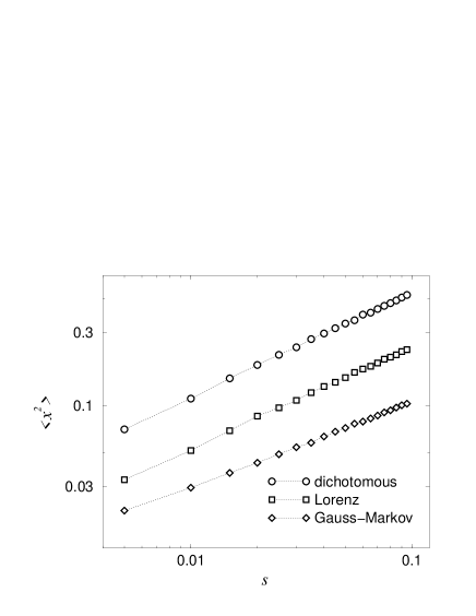
FIG. 8.: Second moments $<x^{2}>$ vs. the strength $s$ of the additive noise calculated for dichotomous noise, Gauss-Markov noise, and Lorenz noise. The value of $\lambda_{0}$ is $-0.5$ for the dichotomous and Gauss-Markov noise, and $-0.3$ for the Lorenz noise. Each line is shifted upwards or downwards to avoid overlap.

VI Some related systems

A Noisy on-off intermittency

Since noisy on-off intermittency is a typical phenomenon with the mechanism of generating the power law of moments, we briefly discuss it here.

On-off intermittency is observed where a chaotic attractor becomes marginally stable with respect to disturbances transversal to the invariant manifold in which the chaotic attractor is embedded. This type of instability is called a blowout bifurcation. The system then alternates between two phases intermittently: a laminar phase where the system stays practically on the invariant manifold, and a burst phase where the deviation from the invariant manifold grows suddenly. The mechanism responsible for the on-off intermittency is that the distance between the orbit and the invariant manifold is governed by a multiplicative process with a chaotically changing multiplier. Therefore, the corresponding suitable mathematical model is a RMP, where the fast chaotic motion of the multiplier is considered as a multiplicative noise.

Platt et al. [4] investigated a situation where weak additive noise is also present in the system. They found that the intermittency, which was originally observed only in a narrow supercritical-side region of the blowout bifurcation, can be observed in a wider region including the subcritical side of the blowout bifurcation. This is called noisy on-off intermittency. In order to explain this phenomenon, they proposed a RMP model which incorporates the effect of the additive noise approximately by introducing a lower bound to the conventional model of on-off intermittency. Venkataramani et al. [5] and Čenys et al. [6] also analyzed similar models and explained some features of the noisy on-off intermittency. However, the power law of moments which we described above has not fully been investigated. Thus, we give an example below.

B Coupled chaotic elements

Two identical chaotic elements coupled with each other [1] is a typical system which shows on-off intermittency. A frequently used model is

$$\left\{\begin{array}[]{rcl}{\dot{\mbox{\boldmath$X$}}_{1}}&=&{\mbox{\boldmath$F$}}({\mbox{\boldmath$X$}}_{1})+k({\mbox{\boldmath$X$}}_{2}-{\mbox{\boldmath$X$}}_{1})\\ \\ {\dot{\mbox{\boldmath$X$}}_{2}}&=&{\mbox{\boldmath$F$}}({\mbox{\boldmath$X$}}_{2})+k({\mbox{\boldmath$X$}}_{1}-{\mbox{\boldmath$X$}}_{2})\end{array}\right.,$$ (70)

where ${\dot{\mbox{\boldmath$X$}}}={\mbox{\boldmath$F$}}({\mbox{\boldmath$X$}})$ gives the dynamics of the individual element, and $k$ the coupling strength. These two elements synchronize with each other when $k$ is larger than a certain critical coupling strength $k_{c}$. The difference ${\mbox{\boldmath$x$}}={\mbox{\boldmath$X$}}_{2}-{\mbox{\boldmath$X$}}_{1}$ is driven multiplicatively by the chaotic motion of the elements as

$${\dot{\mbox{\boldmath$x$}}}=\left[D{\mbox{\boldmath$F$}}(\frac{{\mbox{\boldmath$X$}}_{1}+{\mbox{\boldmath$X$}}_{2}}{2})-2k{\mbox{\boldmath$I$}}\right]\cdot{\mbox{\boldmath$x$}}+O({\mbox{\boldmath$x$}}^{2}),$$ (71)

where $D$ means differentiation and $I$ the unit matrix. Slightly below $k_{c}$, $x$ exhibits on-off intermittency. If we further apply some weak additive noise, $x$ exhibits intermittent behavior above $k_{c}$ as well. If we vary the strength of the additive noise and measure the $q$-th moment $<x^{q}>$ of a certain component of $x$, it is expected to behave like $<x^{q}>$$\simeq G_{0}+G_{1}s^{H(q)}$ as far as $s$ is sufficiently small.

As an example, we numerically calculate a pair of Rössler oscillators coupled with each other, and with weak additive noise applied only to the first component of the state variables:

$$\left\{\begin{array}[]{rcl}\dot{x}_{1}(t)&=&-y_{1}+z_{1}+k(x_{2}-x_{1})+s\xi_{1}(t)\\ \\ \dot{y}_{1}(t)&=&x_{1}+0.3y_{1}+k(y_{2}-y_{1})\\ \\ \dot{z}_{1}(t)&=&0.2+x_{1}z_{1}-5.7z_{1}+k(z_{2}-z_{1})\end{array}\right.,$$ (72)

and

$$(1\longleftrightarrow 2),$$ (73)

where $\xi_{1,2}(t)$ are Gaussian-white noise of average $0$ and variance $1$, and $s$ controls their strength. We set the coupling strength $k$ to the value slightly above $k_{c}$, where the system shows noisy on-off intermittency. Figure 9 shows second moments $<x^{2}>$ of the difference between the first components $x=x_{2}-x_{1}$ versus the noise strength $s$, obtained for some values of the coupling strength $k$. As expected, they show power-law dependence on $s$, and their exponents vary with $k$.

We also observed the power law of moments in a system of coupled chaotic elements with a slight parameter mismatch [2] in place of a weak additive noise, where the parameter mismatch plays a role similar to the additive noise. The power law of moments is also observed in systems of coupled maps [14].

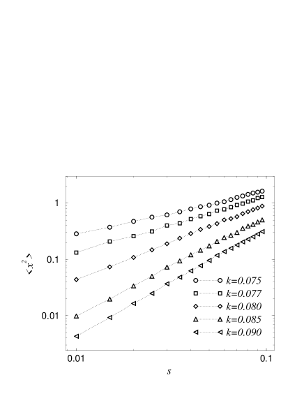
FIG. 9.: Second moments $<x^{2}>$ vs. the strength $s$ of the additive noise of coupled Rössler oscillators obtained for several values of $k$.

C Spatially distributed chaotic elements

The power-law spatial correlation which we studied in the previous papers [12, 13] turns out to be the same as the power law described above, with a proper physical interpretation of some variables involved. The systems we treated previously are the populations of spatially distributed chaotic elements. The elements are driven by a field produced by non-local coupling, which is spatially long-waved and temporally irregular.

If we consider the difference $x(r)=X(r)-X(0)$ between the amplitude $X$ of two elements which are separated by a short distance $r$, its moments $<x(r)^{q}>$ are directly related to the spatial correlations of $X$. They are similar to the structure functions in the context of fluid turbulence or the height-height correlations in the context of fractal surface growth. The dynamics of $x(r)$ is given by a RMP with a weak additive noise, where the multiplier is the local Lyapunov exponent fluctuating randomly due to the chaotic motion of the elements, and the weak additive noise comes from the small difference in the strength of the applied field between the two points under consideration.

Since the strength $s$ of the additive noise should be of the order of $r$ due to the assumed smooth spatial variation of the applied field, the power law of moments as a function of $s$ is now interpreted as a power law of moments of the amplitude difference $x$ as a function of the mutual distance $r$, i.e.,

$$<x(r)^{q}>\sim G_{0}+G_{1}s^{H(q)}\sim G_{0}+G_{2}r^{H(q)},$$ (74)

where $G_{0}$, $G_{1}$, and $G_{2}$ are constants.

When the average Lyapunov exponent is negative, $G_{0}$ vanishes and the exponent $H(q)$ is given by Eq. (31). It shows a “bifractality” similar to that known for Burgers equation, which implies an underlying intermittent structure.

VII Conclusion

As in the models for noisy on-off intermittency and economic activity, a stochastic process driven by multiplicative and weak additive noise shows a power-law PDF. The PDF consists of a constant part and a power-law part, and their boundary moves with the strength $s$ of the additive noise in such a way that its distance from the origin is proportional to $s$. This systematic dependence on $s$ causes the power law of the moments with respect to the strength of the additive noise.

In order to study this phenomenon in further detail, we introduced a Langevin equation (1) with multiplicative and additive noise terms as a general model for a stochastic process of this type. We analyzed its stationary state theoretically and numerically, and found that this model actually reproduces the power law of moments. Furthermore, by comparing the approximate and exact treatments of the effect of the additive noise, the usual approximation of the additive noise by introducing a lower bound of the amplitude was justified.

Although we restricted our study to the Langevin equation (1) for the sake of precise argument, the power law itself is not sensitive to the details of the model employed, and can appear robustly in many stochastic processes driven by multiplicative and weak additive noise. We demonstrated such robustness numerically for some different models, where the system is driven by noises which are not Gaussian-white. Furthermore, as some typical realizations of this type of power law, we discussed the power law of moments in noisy on-off intermittency, and the power-law spatial correlation functions in the spatio-temporal chaotic regime of non-locally coupled systems, which gives some more insight into the power law of the spatial correlation function.

As we already noted, the power law of moments seems to be a general phenomenon appearing in various systems over a wide range of parameters. This mechanism of generating a power law seems to be quite universal, and some of the power laws observed in the real world may belong to this class.

- [1] H. Fujisaka and T. Yamada, Prog. Theor. Phys. 74, 918 (1985)
- [2] T. Yamada and H. Fujisaka, Phys. Lett. A 124, 421 (1987)
- [3] A. S. Pikovsky, Phys. Lett. A 165, 33 (1992)
- [4] N. Platt, S. M. Hammel, and J. F. Heagy, Phys. Rev. Lett. 72, 3498 (1994)
- [5] S. C. Venkataramani, T. M. Antonsen Jr., E. Ott, and J. C. Sommerer, Physica D 96, 66 (1996)
- [6] A. Čenys, A. N. Anagnostopoulos, and G. L. Bleris, Phys. Lett. A 224, 346 (1997); A. Čenys and H. Lustfeld, J. Phys. A 29, 11 (1996)
- [7] R. Graham, M. Höhnerbach, and A. Schenzle, Phys. Rev. Lett. 48, 1396 (1982); A. Schenzle and H. Brand, Phys. Rev. A 20, 1628 (1979)
- [8] M. Levy and S. Solomon, Int. J. Mod. Phys. C 7, 595 (1996)
- [9] H. Takayasu, A-H. Sato, and M. Takayasu, Phys. Rev. Lett. 79, 966 (1997)
- [10] M. Turelli, Theor. Pop. Biol. 12, 140 (1977)
- [11] J. M. Deutsch, Physica A 208, 445 (1994); Physica A 208, 433 (1994)
- [12] Y. Kuramoto and H. Nakao, Phys. Rev. Lett. 76, 4352 (1996)
- [13] Y. Kuramoto and H. Nakao, Phys. Rev. Lett. 78, 4039 (1997)
- [14] T. Mishiro, in preparation.