The Anisotropic Bak–Sneppen Model

Abstract

The Bak–Sneppen model is shown to fall into a different universality class with the introduction of a preferred direction, mirroring the situation in spin systems. This is first demonstrated by numerical simulations and subsequently confirmed by analysis of the multi–trait version of the model, which admits exact solutions in the extremes of zero and maximal anisotropy. For intermediate anisotropies, we show that the spatiotemporal evolution of the avalanche has a power law “tail” which passes through the system for any non–zero anisotropy but remains fixed for the isotropic case, thus explaining the crossover in behaviour. Finally, we identify the maximally anisotropic model which is more tractable and yet more generally applicable than the isotropic system.

64.60.Lx, 05.40.+j, 05.70.Jk

Accepted for publication in J. Phys. A

I Introduction

The Bak–Sneppen model was originally introduced as a crude caricature of biological macroevolution in an attempt to explain the distribution of extinction sizes observed in the fossil record [1, 2, 3]. Although still widely studied in this context, there is also a great deal of interest in analysing the model from a purely abstract viewpoint. This is because it is currently the simplest and most tractable of the class of extremal dynamical models, which themselves form a subset of self–organised critical systems [2, 4, 5]. Extremal dynamical models are so called because they are driven by the the selection of some globally extremal value which dynamically interacts with nearby sites. They naturally evolve towards a “critical state” (a second order phase transition) without any characteristic length or time scales.

It might appear that the Bak–Sneppen model is well suited to adopt the rôle of the “Ising model” of extremal dynamical systems. We believe that this is not the case, and in this paper we detail an even simpler version of the model which is more open to analysis whilst retaining all the essential behaviour of the original. The inspiration behind this new model can be most clearly described by analogy with spin systems [6]. The Heisenberg spin model is isotropic because the spin vectors have no preferred direction. However, when even the slightest anisotropy is introduced, a preferred direction is created and the system falls into a different universality class. Furthermore, this is the same class as the highly anisotropic Ising model, where the spin vectors can only lie parallel to the direction of quantisation. So not only is the Ising model in some sense more general than the Heisenberg model, it is also simpler and hence more tractable.

The original incarnation of the Bak–Sneppen model is like the Heisenberg model in that it too is isotropic. If the analogy with spin systems is to hold true, then the introduction of anisotropy into the Bak–Sneppen model should result in a different universality class. We find that this is indeed the case, at least for one dimensional systems, and conclude that, unless there is some reason for assuming perfect isotropy, it is the anisotropic model that should be treated as the general case and the isotropic version as a special limiting instance. It is also possible to identify a maximally anisotropic Bak–Sneppen model which may serve as the true analogue of the Ising model for extremal dynamical systems. We postpone until Sec.V the question of whether isotropy should be assumed in any known application of the model.

This paper is organised as follows. Numerical simulations of anisotropic systems are described in Sec. II and the exponents for the new universality class are given. By switching to the multi–trait model, a full solution of the maximally anisotropic system is found which explicitly demonstrates the crossover to the new class. This solution is derived in Sec. III alongside the known result for the isotropic model. An exact solution for intermediate anisotropies was not forthcoming, but by employing an alternative means of analysis it is possible to show that this new class also applies to any non–zero anisotropy. This is presented in Sec. IV. Finally, in Sec. V we discuss the applicability of this new class in real situations, and consider the potential of the maximally anisotropic model in future analytical treatments.

II The Anisotropic Model

Before coming to consider anisotropy we briefly summarise the isotropic model and some of its known results [1, 2]. $N$ scalars $f_{i}$ , where $i=1\ldots N$ , are placed on a one–dimensional lattice with periodic boundary conditions. The $f_{i}$ , known as “barriers,” are random numbers uniformly distributed on $[0,1]$, although the system behaves in essentially the same manner regardless of the particular choice of distribution. At each time step the global minimum of all the $f_{i}$ is found, and it and its two nearest neighbours are given new random values from the same distribution as before. This process is then repeated ad infinitum.

Despite such minimalist dynamics the model exhibits a rich variety of non–trivial behaviour. It evolves towards a statistical steady state in which the bulk of the $f_{i}$ are uniformly distributed on $[f_{c},1]$, where the threshold value $f_{c}$ is a function of the lattice dimension and connectivity. For the one–dimensional lattice considered here, $f_{c}\approx 0.667$. A finite number of barriers form a tail on $[0,f_{c}]$ and it is in this tail that the global minimum is always to be found. Both the spatial and temporal correlation functions are power law in form, signifying the existence of a critical state with no characteristic length or time scales. The distribution for the absolute distance between successive minima $\Delta x$ is

$$P_{\rm JUMP}(\Delta x)\sim(\Delta x)^{-\pi}\>,$$ (1)

where $\pi=3.23\pm 0.02$. The probability that the minimum is at the same site at times $t_{0}$ and $t+t_{0}$ is given by

$$P_{\rm ALL}(t)\sim t^{-\tau_{\rm ALL}}\>,$$ (2)

with $\tau_{\rm ALL}=0.42\pm 0.02$. This holds true as long as $t\ll t_{0}$ and ageing effects can be ignored [7, 8].

The model defined above is isotropic because the interaction between the global minimum and the other barriers is the same in both directions. In other words, if the current minimum is $f_{i}$ then barriers $f_{i-1}$, $f_{i}$ and $f_{i+1}$ are reset, so the minimum is just as likely to jump to the left as it is to the right. Consider what happens when the rules are altered so that $f_{i-1}$, $f_{i}$ and $f_{i+2}$ are reset instead. The system now has an inherent bias to the right and we would expect an avalanche to be more likely to propagate in that direction. This constitutes an anisotropic model since there now exists a preferred direction for the global minimum to drift.

We have performed extensive numerical simulations of the anisotropic model and have observed that the system behaves in qualitatively the same manner as the isotropic model. However, the correlation distributions $P_{\rm JUMP}$ and $P_{\rm ALL}$ have different exponents, $\pi^{\uparrow}=2.42\pm 0.05$ and $\tau^{\uparrow}_{\rm ALL}=0.59\pm 0.03$, so the system falls into a different universality class to the isotropic case. Plots of $P_{\rm ALL}$ for both classes are given in Fig. 1 for direct comparison. $P_{\rm JUMP}$ is uniformly lower for jumps against the direction of anisotropy as for jumps with it, but the same exponent applies in both directions. The threshold value $f_{c}$ also drops, but this is simply due to the increased spreading out of the avalanche and has nothing to do with the loss of isotropy.

The new universality class is not just restricted to this one example. Simulations have shown that if barriers $f_{i-a}$, $f_{i}$ and $f_{i+b}$ are reset, where $a$ and $b$ are arbitrary positive integers, then the same class holds for any $a\neq b$. The dynamics can be further generalised by considering ranges of sites on each side of the minimum, and either selecting all of these sites or just a random sample. Here, anisotropy corresponds to a larger range on one side than on the other. In all cases the same exponents are found for any non–zero anisotropy, although convergence can be very slow when the anisotropy is weak, a point that will be explicitly demonstrated for the multi–trait model in Sec. IV.

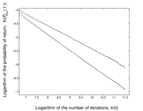
FIG. 1.: A log–log plot of $P_{\rm ALL}(t)$, the probability for the active site to return to its original position after a time $t$. The upper line is from the standard isotropic model and the lower line is from an anisotropic system in which the barriers $f_{i-1}$, $f_{i}$ and $f_{i+3}$ are reset at every time step, where $f_{i}$ is the current global minimum. The dashed lines have slopes of $-0.42$ and $-0.59$, respectively. The data for the anisotropic system has been moved upwards to allow for direct comparison with the isotropic case. The simulations were performed on an $N=10^{4}$ lattice, for $5\times 10^{3}N$ iterations in the isotropic case and $5\times 10^{4}N$ in the anisotropic case.

III The Multi–Trait Model

The consequences of introducing anisotropy into the Bak–Sneppen model can be more fully investigated by switching to the multi–trait framework [9]. In the multi–trait model each site has $M$ internal degrees of freedom, that is $M$ different barriers rather than just the usual 1. At each time step the smallest of all the $N\times M$ barriers in the system is found and reset. One of the $M$ barriers from each of its neighbouring sites is selected at random and also reset, so three barriers are reset in total. Then the new global minimum is found and the process is iterated indefinitely. For finite $M$ the system belongs to the same universality class as the standard $M=1$ model, but for $M\rightarrow\infty$ it falls into a different class and, furthermore, can be solved exactly. To see why this is so, we must first define what is meant by a $\lambda$–avalanche.

For any given value of $\lambda<f_{c}$ the global minimum can be either greater or less than $\lambda$. Hence a time series of the minimum will consist of regions where it is less than $\lambda$ alternating with regions where it is greater than $\lambda$. Each block for which the global minimum is less that $\lambda$ is defined as a $\lambda$–avalanche. During a $\lambda$–avalanche any barrier smaller than $\lambda$ is called active since the avalanche cannot finish until all of the active barriers have been made inactive, that is when they have all been reset to values greater than $\lambda$. There are only two ways in which a barrier can get reset, it either becomes the global minimum or belongs to an adjacent site to the minimum and is selected with probability $1/M$. However, the latter possibility cannot occur in the $M\rightarrow\infty$ limit since there are only a finite number of active barriers in the system at any one time, so the probability of selecting one at random is vanishingly small. Hence each active barrier must eventually become the global minimum and it will then initiate a sub–avalanche that can change inactive barriers to active, but never the other way around. Furthermore, since the sub–avalanches from different active barriers propagate independently of each other, the active barriers can be reset in any order and there is no longer any need to keep track of which is actually the global minimum.

The temporal correlations for $M\rightarrow\infty$ are the same as for a mean field model in which the neighbours of the minimum are chosen at random, so the introduction of anisotropy will make no difference. Rather than repeat the analysis here, we simply quote the main result and refer the reader to [9] for details of the derivation. If $P_{\lambda}(t)$ is the probability that a $\lambda$–avalanche lasts for exactly time $t$, then

$$P_{\lambda}(t)\sim t^{-3/2}\;G(\;t\,(\lambda-\mbox{$\frac{1}{2}$})^{2}\,)$$ (3)

as $\lambda\rightarrow f_{c}=\frac{1}{2}$, where $G(x)$ is a scaling function that tends to a constant value for $x\rightarrow 0$. As expected, $P_{\lambda}$ has the usual mean field exponent of $\frac{3}{2}$. Since (3) holds independently of the spatial structure of the system, we can already conclude that the threshold barrier value $f_{c}$ will be $\frac{1}{2}$ regardless of the degree of anisotropy.

Anisotropy will clearly effect the spatial correlations and so we present the following analysis in some detail, starting with the isotropic model. As in the derivation of (3) the algebra is simplified by stipulating that the active barrier always takes the value of 1 when it is reset. This makes no qualitative difference to the results. Hence the central barrier is always made inactive, but the barriers reset in each of the adjacent sites may become active with probability $\lambda$. Let $g_{r}$ denote the probability that resetting an active barrier at the origin causes at least one of the barriers in site $r$ to become active. Then $1-g_{r}$ is the probability that no barriers become active, which can be related to $1-g_{r-1}$ and $1-g_{r+1}$ by the difference equation

$$1-g_{r} = (1-\lambda)^{2}+\lambda^{2}(1-g_{r-1})(1-g_{r+1})$$ (5)

$$\mbox{}+\lambda(1-\lambda)\left\{(1-g_{r-1})+(1-g_{r+1})\right\}\>.$$

This can be derived by considering what happens when an active barrier at the origin is reset. The probability of creating no new active barriers is $(1-\lambda)^{2}$, in which case the avalanche will end and site $r$ will definitely not become active. This is catered for by the first term on the right hand side of (5). Similarly, the second and third terms account for the creation of active barriers in one or both of the adjacent sites, which may subsequently propagate to site $r$ with probabilities $g_{r-1}$ and $g_{r+1}$, assuming $g_{r}$ to be translationally invariant. (5) can be rearranged to give

$$g_{r}=\lambda(g_{r-1}+g_{r+1})-\lambda^{2}g_{r-1}g_{r+1}\>.$$ (6)

If the whole $\lambda$–avalanche starts from a single active barrier at $r=0$, then $g_{0}=1$ and (6) can be solved to give

$$g_{r}=\frac{12}{(r+3)(r+4)}$$ (7)

for $\lambda=\frac{1}{2}$ , explicitly demonstrating the asymptotic power law behaviour $g_{r}\sim 1/r^{2}$.

There are many ways in which anisotropy could be incorporated into this framework, but for clarity we restrict our attention to just a single definition. At every time step the global minimum barrier is found, say in site $i$, and reset. The anisotropic interaction consists of randomly selecting one of the $M$ barriers in each of the sites $i-a$ and $i+b$ and resetting them both, where the parameters $a$ and $b$ are positive integers. Some examples are given in Fig. 2. Note that if $a$ and $b$ share a common factor, say $c$, then the system will trivially decouple into $c$ independent sublattices. For instance, if $a=b=2$ then all the even numbered sites will decouple from all the odd numbered sites and the two sublattices will evolve independently of each other. Thus we can safely assume that $a$ and $b$ are coprime. As a corollary any system with $a=b$ is equivalent to the standard model $a=b=1$. Similarly, if $a$ is equal to zero we can take $b=1$ without loss of generality, and vice versa if $b=0$.

The maximally anisotropic system with $a=0$ and $b=1$ can be solved in much the same way as the isotropic case. Since only two barriers are reset at every time step anyway there is no need to set the central barrier to 1 as before. The resulting difference equation is similar to (5) and can be derived in an entirely analogous manner,

$$1-g_{r} = (1-\lambda)^{2}+\lambda^{2}(1-g_{r})(1-g_{r+1})$$ (9)

$$\mbox{}+\lambda(1-\lambda)\left\{(1-g_{r})+(1-g_{r+1})\right\}\>,$$

which rearranges to

$$g_{r}=\frac{\lambda g_{r-1}}{1-\lambda+\lambda^{2}g_{r-1}}\>.$$ (10)

For $\lambda=\frac{1}{2}$ this admits the exact solution

$$g_{r}=\left\{\begin{array}[]{ll}\frac{2}{2+r}&\mbox{ for $r\geq 0$, and}\\ 0&\mbox{for $r<0$,}\end{array}\right.$$ (11)

so now $g_{r}\sim 1/r$ for large $r$, giving a power law with an exponent of $1$.

An exact expression for $\lambda\neq\frac{1}{2}$ can also be found by substituting $g_{r}=1/z_{r}$ into (10). This gives a linear difference equation for the $z_{r}$,

$$z_{r}=\frac{1-\lambda}{\lambda}\;z_{r-1}+\lambda\>,$$ (12)

which can be solved to give

$$z_{r}=\frac{\lambda^{2}}{1-2\lambda}\left\{\left(\frac{1-\lambda}{\lambda}\right)^{r+2}-1\right\}\>.$$ (13)

For $\lambda<\frac{1}{2}$, $z_{r}$ blows up exponentially in $r$ and so $g_{r}$ will exponentially decay to zero. If $\lambda>\frac{1}{2}$ then $g_{r}$ will exponentially decay to a constant value for large $r$, corresponding to a non–zero probability of initiating an infinite avalanche. However, this latter case is of academic interest only since the underlying simplification of the $M\rightarrow\infty$ limit rests on there being only a finite number of active barriers at any one time, which is no longer true when $\lambda>\frac{1}{2}$ .

The exponent for $g_{r}$ is related to the exponent for $P_{\rm JUMP}$ by $\pi=\tau_{\rm R}+1$, where $g_{r}\sim r^{-\tau_{\rm R}}$ and $P_{\rm JUMP}(\Delta x)\sim(\Delta x)^{-\pi}$. Hence the analysis given above demonstrates that $\pi$ changes from 3 to 2 with the introduction of anisotropy. This should be compared to the numerical results in Sec. II for $M=1$ systems, where $\pi$ went from $3.23\pm 0.02$ to $2.42\pm 0.05$. In both cases the exponent jumps in the same direction and by a roughly similar amount. Furthermore, for $M\rightarrow\infty$ the exponent for $P_{\rm ALL}(t)\sim t^{-\tau_{\rm ALL}}$ obeys $\tau_{\rm ALL}=(2\tau_{\rm R})^{-1}$. Hence $\tau_{\rm ALL}$ increases from $\frac{1}{4}$ to $\frac{1}{2}$, and again a similar jump was observed for $M=1$, where $\tau_{\rm ALL}$ increased from $0.42\pm 0.02$ to $0.59\pm 0.03$. Thus the change in behaviour in the $M\rightarrow\infty$ limit is also representative of the $M=1$ case.

FIG. 2.: Examples of various definitions of anisotropy. In all cases the solid square is the site with the global minimum and the shaded squares are the other sites in which a barrier is also reset. The shaded sites are $a$ places to the left of the site with the minimum, and $b$ places to its right. (a) The standard model $a=b=1$. (b) The maximally anisotropic model $a=0$, $b=1$. (c) An intermediate case $a=2$, $b=3$.

IV Arbitrary Anisotropy

It remains to be seen whether systems with intermediate anisotropies do indeed fall into the same universality class as the maximally anisotropic model, as implied by the analogy with the Heisenberg and Ising spin models. Unfortunately, the style of analysis adopted in the previous section is of little use here since the difference equation (6) admits no straightforward solutions for arbitrary $a$ and $b$. The difficulty stems from the fact that the interactions are now between non–adjacent sites. One way around this problem is to find a separate lattice representation for the avalanche in which only nearest neighbours interact. This could then be mapped onto the one–dimensional substrate in such a way that nearest neighbours on the avalanche lattice map onto interacting sites on the substrate.

To do this unambiguously, it is necessary to employ a two–dimensional lattice $(n,m)$ which represents the entire spatiotemporal extent of the avalanche. The mapping from sites $(n,m)$ on the avalanche lattice to sites $r$ on the one–dimensional substrate is derived as follows. The origin $(0,0)$ corresponds to $r=0$. Any given site $(n,m)$ can be reached by taking $n$ steps to the left and $m$ steps to the right, in any order. For arbitrary $a$ and $b$, the resulting value of $r$ is

$$r=na-mb\>.$$ (14)

Each value of $r$ corresponds to the set of points $(n_{i},m_{i})$ that obey (14). Successive points are separated by the constant displacement vector

$$\Delta_{nm} = (n_{i+1},m_{i+1})-(n_{i},m_{i})$$ (15)

$$= (n_{i+1}-n_{i},m_{i+1}-m_{i})$$ (16)

$$= (b,a)\>.$$ (17)

That $\Delta_{nm}$ is the smallest displacement vector follows from the coprime nature of $a$ and $b$. The mapping from $(n,m)$ to $r$ can thus be regarded as a projection from the two–dimensional avalanche lattice to the one–dimensional substrate. An example is given in Fig. 3(a) for the isotropic model. When $a\neq b$ the $(n,m)$–lattice becomes rotated relative to the projection lines, so for instance when $a=0$ and $b=1$ the lattice lies completely on its side, as in Fig. 3(b). An intermediate case is given in Fig. 3(c).

FIG. 3.: The projection from the $(n,m)$ lattice to sites $r$ on the one-dimensional substrate. Adjacent sites on the $(n,m)$ lattice correspond to sites $r$ that interact. (a) The isotropic model $a=b=1$. The dotted lines connect all the $(n,m)$ that correspond to the same value of $r$. (b) The maximally anisotropic case $a=0$, $b=1$. (c) An intermediate case $a=2$, $b=1$.

To quantify this relationship further, let $p_{nm}$ be the probability that site $(n,m)$ is active. Site $r$ will remain inactive throughout the entire avalanche only if all of its corresponding $(n,m)$ are also inactive, so

$$g_{r}=1-\prod_{n,m}(1-p_{nm})\>,$$ (18)

where the product is taken over all the $n$ and $m$ that obey (14). The advantage of this approach is that varying the anisotropy only effects which $p_{nm}$ contribute to (18), the $p_{nm}$ themselves are entirely unaltered. Thus a unique solution to the $p_{nm}$ exists which, if found, could be applied to any anisotropy through (18) without modification.

The next step is to find the solution for the $p_{nm}$. Each site $(n,m)$ has $M$ barriers which, if active, may create active barriers in either or both of sites $(n+1,m)$ and $(n,m+1)$. Since we are still in the $M\rightarrow\infty$ limit, the sub–avalanches initiated by different active barriers are independent and can be arranged so as to form a compact avalanche on the $(n,m)$ lattice. A site $(n,m)$ can only become active if one of its barriers is reset to a value less that $\lambda$ due to the interaction with an active neighbouring site. The neighbours in question are the two diagonally lower sites $(n-1,m)$ and $(n,m-1)$, so the probability of either event occurring independently is $\lambda\,p_{n-1m}$ and $\lambda\,p_{nm-1}$, respectively. Thus the difference equation for the $p_{nm}$ is

$$p_{nm}=\lambda(p_{n-1m}+p_{nm-1})-\lambda^{2}p_{n-1m}p_{nm-1}\>.$$ (19)

By dropping the second term on the right hand side of (19), a linear equation is obtained which has the exact solution

$$p^{\rm lin}_{nm}=\frac{(n+m)!}{n!\,m!}\,\lambda^{n+m}\>.$$ (20)

Except for a missing normalisation factor of $2^{-(n+m)}$, the coefficients $(n+m)!/(n!\,m!)$ describe a binomial distribution with equal probability of either outcome. For large $n$ and $m$ this binomial is well approximated by a Gaussian distribution with mean $(n+m)/2$ and variance $(n+m)/4$ ,

$$p^{\rm lin}_{nm}\approx\sqrt{\frac{2}{\pi(n+m)}}\,\exp\left\{{-\frac{1}{2}\frac{(n-m)^{2}}{n+m}}\right\}\,(2\lambda)^{n+m}\>.$$ (21)

This expression is vanishingly small except for points that lie near the line $n=m$, which form a non–vanishing “tail”. A cut through points of equal $n+m$ shows that this tail has a Gaussian cross section of width $\frac{1}{2}\sqrt{n+m}$ , so it becomes broader down its length. The behaviour down the centre of the tail depends upon the value of $\lambda$. For $\lambda\neq\frac{1}{2}$, $p^{\rm lin}_{nn}$ either blows up or decays exponentially according to the factor of $(2\lambda)^{2n}$ in (21). At the critical point $\lambda=\frac{1}{2}$ this factor becomes unity and instead the tail exhibits power law decay $p^{\rm lin}_{nn}\sim n^{-1/2}$.

Numerical integration of the full difference equation (19) shows that the exact solution of $p_{nm}$ does indeed have a Gaussian tail of variance $(n+m)/4$ which decays as a power law for $\lambda=\frac{1}{2}$, in agreement with the expression for $p^{\rm lin}_{nm}$. However, the exponent for the power law decay is different in both cases, $p_{nn}\sim n^{-1}$ for the exact solution as opposed to $p^{\rm lin}_{nn}\sim n^{-1/2}$. The correct exponent can be recovered by restoring the non-linear term in (19) and instead considering the equivalent continuum approximation [10]. Let $x$ and $y$ be continuous variables corresponding to $n$ and $m$, and define $h(x,y)=p_{nm}$. Using this notation,

$$\nabla h(x,y) = \frac{\partial h(x,y)}{\partial x}+\frac{\partial h(x,y)}{\partial y}$$ (22)

$$\approx (p_{nm}-p_{n-1m})+(p_{nm}-p_{nm-1})\>,$$ (23)

and (19) can be rewritten as

$$\frac{1}{2}\nabla h=(2\lambda-1)h-\lambda^{2}h^{2}\>.$$ (24)

This can be simplified by making the substitution $h(x,y)=1/z(x,y)$ and the change of variables $u=x+y$ and $v=x-y$, giving

$$\frac{\partial z}{\partial u}=(1-2\lambda)\,z+\lambda^{2}\>.$$ (25)

For $\lambda=\frac{1}{2}$ the first term on the right hand side of (25) vanishes and straightforward integration gives

$$z(u,v)=\frac{u}{4}+A(v)\>,$$ (26)

where $A(v)$ is an arbitrary function of $v$ that is found from the boundary conditions. There are two sets of boundary conditions, one for the line $m=0$ and another for the line $n=0$. It is clear from (19) that $p_{n0}=\lambda^{n}$ exactly. The line $m=0$ is the same as the line $y=0$, which maps onto $u=v$ after the change of variables, so the first boundary condition is $z(u,u)=\lambda^{-u}$. Similarly, $p_{0m}=\lambda^{n}$ and the line $n=0$ corresponds to $u=-v$, so the second boundary condition is $z(u,-u)=\lambda^{-u}$. This allows for $A(v)$ to be fixed and the full solution is

$$z(u,v)=\frac{u-|v|}{4}+2^{|v|}\>.$$ (27)

Along the tail $v=0$, $z(u,0)\sim u$ and so $h(x,x)\sim x^{-1}$, giving the correct exponent for the decay. However, moving away from the tail results in exponential growth in $z(u,v)$ and hence exponential decay in $h(x,y)$. Thus the continuum approximation predicts the correct exponent for the decay of the tail but the wrong cross sectional shape, that is, exponential rather than Gaussian.

The solution for $\lambda<\frac{1}{2}$ can be found by following exactly the same procedure. This results in

$$z(u,v)=\frac{\left((1-2\lambda)\lambda^{-|v|}+\lambda^{2}\right)e^{(1-2\lambda)(u-|v|)}-\lambda^{2}}{1-2\lambda}\>.$$ (28)

As before, this expression increases exponentially away from the tail. For $v=0$ it reduces to

$$z(u,0)=\frac{(1-\lambda)^{2}e^{(1-2\lambda)u}-\lambda^{2}}{1-2\lambda}\>,$$ (29)

which blows up exponentially in $u$. Hence $h(x,x)$ decays to zero when $\lambda<\frac{1}{2}$ , giving an exponential cut-off in the distribution of avalanche sizes. We note in passing that (28) also holds for $\lambda>\frac{1}{2}$ but, as explained in the Sec. III, such values of $\lambda$ bear no relevance to actual systems.

Armed with the solution to the $p_{nm}$ , we can now derive the exponents of $g_{r}$ for when $\lambda=\frac{1}{2}$. First consider the isotropic case $a=b=1$. Under the projection in Fig. 3(a) all the points down the centre of the tail are mapped onto the origin, so $g_{r\neq 0}$ will only start to receive non-vanishing contributions once the tail has become sufficiently wide. Since the tail broadens like $(n+m)^{1/2}$ the first $p_{nm}$ to contribute to $g_{r}$ will lie on the line $n+m\sim r^{2}$, by which point the tail will have already decayed to $p_{nm}\sim(n+m)^{-1}\sim r^{-2}$. Once these $p_{nm}$ are substituted into the infinite product in (18), the leading order terms in $g_{r}$ will look something like

$$g_{r}\approx\frac{a_{2}}{r^{2}}+\frac{a_{4}}{r^{4}}+\frac{a_{6}}{r^{6}}+\ldots\>\>\>,$$ (30)

where the $a_{i}$ are constants. Hence $g_{r}=O(1/r^{2})$, in agreement with the exact solution (7).

The situation is very different in an anisotropic system $a\neq b$. As can be seen in Figs. 3(b) and 3(c), the tail is no longer vertical but cuts through the projection lines at a finite angle, passing over all $r\geq 0$ (the preferred direction is to the right in both of these examples). Furthermore, since the gap between successive $p_{nm}$ mapped onto the same $r$ is finite, and the tail broadens without limit, then for sufficiently large $r$ an arbitrarily large number of $p_{nm}$ will contribute to each $g_{r}$. Each of these $p_{nm}$ will be proportional to $1/r$, so the analogous expression to (30) will be $g_{r}=O(1/r)$ and power law behaviour with an exponent of $1$ is recovered, in agreement with (11) and numerical simulations. For $r<0$ only exponentially small $p_{nm}$ contribute and $g_{r<0}$ takes some exponentially decaying form.

Thus the crossover in behaviour from the anisotropic to the isotropic model in the $M\rightarrow\infty$ limit can be attributed to the difference between a power law tail that moves across the substrate, and one whose centre is fixed and can only broaden at a much slower rate. The convergence to the new behaviour can be very slow, especially for weak anisotropy $a\approx b$. Indeed, since $g_{r}\sim 1/r+O(1/r^{2})$ the rate of convergence is itself a power law. Slow convergence was also observed in the simulations of the $M=1$ models is Sec. II. However, for $M=1$ the spatial correlations were power law in both directions, whereas in the $M\rightarrow\infty$ limit the correlations against the direction of anisotropy decay exponentially. This difference presumably arises because the sub–avalanches initiated from different active sites are no longer independent for finite $M$.

V Discussion

It should come as no surprise that the anisotropic Bak–Sneppen model has different critical exponents to its isotropic equivalent. Universality classes depend upon the dimensionality and symmetries of the model in question, so the loss of symmetrical interactions should result in a different class. In spin systems the crossover from Heisenberg to Ising behaviour occurs around a given temperature, which could be very close to the critical temperature for weak anisotropies. There is no direct analogue of temperature in the Bak–Sneppen model, where the critical state is now the attractor of the dynamics, but for weak anisotropies the convergence to the new exponents is very slow. Nonetheless, we believe that it is the anisotropic class which should now be regarded as the general case.

The isotropic model could still have applications in any situation where perfect isotropy can be assumed. The question then becomes, do any such situations exist? In both of the model’s applications we are aware of, we think the answer is clearly ‘no’. In the biological context, asymmetry between coevolving species could occur for a number of reasons. A graphic example for predator–prey relationships is known as the “life/dinner” principle, where the asymmetry arises because the prey has more to lose from a failed encounter than the predator [11]. This gets its name from an Aesop’s fable, where a dog gives up chasing a hare because it is only running for its dinner, whereas the hare is running for its life, hence “life/dinner” principle [12]. Such asymmetry should result in a preferred direction along the food chain, although the issue is somewhat clouded here by the lack of a realistic food web structure [13, 14]. A second application of the model has recently been proposed for the process whereby granular materials, such as sand, powder, corn flakes etc., settle under perturbations [15]. Here, anisotropy would be induced by gravity.

It was mentioned in the introduction that the maximally anisotropic $a=0$, $b=1$ system should be more open to analysis than the isotropic one. This certainly proved to be true in the $M\rightarrow\infty$ limit studied in Sec. III, where exact solutions were found for all values of $\lambda$ rather than just $\lambda=\frac{1}{2}$ , as in the isotropic case. The maximally anisotropic model may also prove to be more tractable in the original $M=1$ framework. This claim is not unreasonable and has many precedents. For instance, the Zaitsev model is an extremal dynamical system with similar rules to the Bak–Sneppen model, except that a random value is subtracted from the global maximum and redistributed equally to its nearest neighbours. Stipulating that this value is instead only distributed in one direction gives rise to an anisotropic variant which can be solved exactly, including explicit expressions for the critical exponents [16]. Another example is provided by the abelian sandpile model, where a version in which the sand only topples in one direction was solved before exact results for the isotropic case were found [17, 18].

One area that we have not investigated is what happens when anisotropy is introduced to lattices with two or more dimensions. This opens up the possibility of having isotropic interactions parallel to one axis but anisotropic interactions parallel to another, the number of permutations between the axes increasing with the dimensionality. Based on the analogy with spin systems, we would expect that there would still be just two universality classes for each dimension, one for the fully isotropic case and one for any non-zero anisotropy. The critical exponents for both classes should converge when the upper critical dimension is reached, beyond which the introduction of anisotropy will make no difference. Work is in progress to find at what dimension this convergence occurs, to help confirm or deny recent claims that the upper critical dimension for the Bak–Sneppen model is 8 [19, 20].

Just prior to publication we became aware of a modified Bak–Sneppen model by Vendruscolo et al. which introduces a preferred direction by a very different mechanism [21]. Nonetheless the critical exponents for their model appear to match those found for our one, which strengthens the case for the universality of the anisotropic class.

REFERENCES

- [1] P. Bak and K. Sneppen, Phys. Rev. Lett. 71, 4083 (1993).
- [2] M. Paczuski, S. Maslov and P. Bak, Phys. Rev. E 53, 414 (1996).
- [3] M. E. J. Newman, J. Theor. Biol. 189, 235(1997).
- [4] M. Marsili, P. De Los Rios and S. Maslov, cond-mat/9710152.
- [5] S. Maslov, Phys. Rev. Lett. 77, 1182 (1996).
- [6] J. M. Yeomans, Statistical Mechanics of Phase Transitions (Oxford Science Publications, Oxford, 1992).
- [7] S. Boettcher and M. Paczuski, Phys. Rev. Lett. 79, 889 (1997).
- [8] S. Boettcher, Phys. Rev. E 56, 6466 (1997).
- [9] S. Boettcher and M. Paczuski, Phys. Rev. Lett. 76, 348 (1996).
- [10] Note that this is the continuum approximation. The continuum limit, achieved by sending the lattice spacing to zero in a suitable manner, is not instructive here since it introduces troublesome delta functions into the boundary conditions.
- [11] R. Dawkins, The Extended Phenotype (Oxford University Press, Oxford, 1982).
- [12] ‘A dog started a hare from a bush, but, practised game-dog though he was, found himself left behind by the scampering of its hairy feet. A goat-herd laughed at him: “Fancy a little creature like that being faster than you.” “It’s one thing”, answered the dog, “running because you want to catch something, but quite another thing running to save your own skin.” ’ From Fables of Aesop, trans. S. A. Handford (Penguin, London, 1954). The protagonists are often misquoted as fox and rabbit.
- [13] S. J. Hall and D. G. Raffaelli, Adv. Ecol. Res. 24, 187 (1993).
- [14] G. Caldarelli, P. G. Higgs and A. J. McKane, adap-org/9801003.
- [15] D. A. Head and G. J. Rodgers, J. Phys. A 31, 107 (1998).
- [16] S. Maslov and Y. Zhang, Phys. Rev. Lett. 75, 1550(1995).
- [17] D. Dhar and R. Ramaswamy, Phys. Rev. Lett. 63, 1659 (1990).
- [18] D. Dhar, Phys. Rev. Lett. 64, 1613 (1990).
- [19] P. De Los Rios, M. Marsili and M. Vendruscolo, preprint cond-mat/9802069.
- [20] D. A. Head and G. J. Rodgers, in preparation.
- [21] M. Vendruscolo, P. De Los Rios and L. Bonesi, Phys. Rev. E 54, 6053(1996).