Inversion of K₃C₆₀ Reflectance Data

Abstract

We outline a procedure for obtaining the electron-phonon spectral density by inversion of optical conductivity data, a process very similar in spirit to the McMillan-Rowell inversion of tunelling data. We assume both electron-impurity (elastic) and electron-phonon (inelastic) scattering processes. This procedure has the advantage that it can be utilized in the normal state. Furthermore, a very good qualitative result can be obtained explicitly, without iteration. We illustrate this technique on recently acquired far-infrared data in K₃C₆₀. We show that the electron-phonon interaction is most likely responsible for superconductivity in these materials.

The determination of the underlying interactions and how they govern the various phases in materials (metallic, insulating, superconducting, etc.) is a major goal in current research of new materials. In the last ten years, both high-T_c oxides and alkali-doped “bucky-balls” (A₃C₆₀, etc.) have provided fascinating cases for study, since several phases are attainable by both doping and temperature variation. The general problem of understanding how these various phases come about is a formidable task, however, and remains unsolved.

In this paper we investigate the origin of superconductivity in K₃C₆₀, a superconducting fullerene with $T_{c}\approx 19$ K. While several experimental facts point towards a conventional electron-phonon mechanism (eg. isotope effect measurements [1, 2] and others — see Refs. [3], [4], [5] and [6] for reviews), the key experiment, which is single electron tunneling at biases above the gap edge, has not yet been performed [7] to the extent that reproducible structure is observed. In fact, definitive results from single electron tunneling may be very difficult to achieve for two reasons. First, the electron-phonon coupling strength may be very weak, in which case the structure will be difficult to observe, and second, neutron scattering experiments indicate that phonon modes are present at very high frequencies [8] ($\omega>200$ meV). If these modes are coupled to the itinerant electrons, then they may be impossible to see through tunneling experiments, whose accuracy becomes less reliable at higher biases.

For these reasons we attempt here to provide as definitive a demonstration of electron-phonon superconductivity as tunneling normally provides, using, however, a higher frequency and potentially more sensitive probe, infrared spectroscopy. This idea is certainly not new, as many years ago Allen [9] provided a rudimentary basis for inferring the electron-phonon spectrum for lead, based on the absorption measurements of Joyce and Richards [10]. This work was followed up by Farnworth and Timusk [11]; they utilized weak coupling expressions due to Allen and were able to extract a spectrum which agreed very well with that obtained from tunneling.

The present work differs somewhat from these approaches in that we utilize only normal state reflectance measurements, over the (in principle) entire frequency range. Through a Kramers-Kronig transformation we obtain the optical conductivity, from which we can deduce the electron-phonon spectrum. We first present some of the theoretical aspects, carry out some checks on Pb, and finally apply our procedure to K₃C₆₀. Our conclusion is that the optical measurements of Degiorgi et al. [12] are consistent with electron-phonon coupling of sufficient strength to drive the superconducting transition in K₃C₆₀.

The starting point is the Kubo formula for the optical conductivity [13] of electrons in a normal metal, at zero temperature:

$$\sigma(\nu)={\omega^{2}_{P}\over 4\pi}{i\over\nu}\int_{0}^{\nu}d\omega{1\over\nu+{i\over\tau}-\Sigma(\omega)-\Sigma(\nu-\omega)}$$ (1)

where

$$\Sigma(\omega)=\int_{0}^{\infty}d\Omega\alpha^{2}F(\Omega)\ln|{\Omega-\omega\over\Omega+\omega}|-i\pi\int_{0}^{|\omega|}d\Omega\ \alpha^{2}F(\Omega)$$ (2)

is the electron self-energy due to the electron-phonon interaction (the term proportional to the electron-impurity scattering rate is explicitly included in Eq. (1)). Eq. (1) has been derived using a number of well-documented approximations: impurity scattering is included in the simplest Born approximation, and electron-phonon vertex corrections have been ignored. Actually we have written the self-energy as a functional of $\alpha^{2}F(\Omega)$, although Allen [9] has noted (following Scher [14]) that this form can be used provided $\alpha^{2}F(\Omega)$ is replaced by a more complicated spectral function called $\alpha^{2}_{ir}F(\Omega)$, which in some limits is very well approximated by $\alpha^{2}_{tr}F(\Omega)$. This latter function contains the essential “$1-cos(\theta)$” factor for transport properties. So, in fact the above equations should contain the transport spectral function, but since this and the usual spectral function are very often qualitatively similar, we have dropped the distinction.

It should be clear from Eqs. (1) and (2) that the normal state conductivity contains an image of the underlying electron-phonon spectral function. This is most apparent if we invoke a weak coupling approximation and expand the denominator in Eq. (1) to first order in the self-energy, so one of the integrals can be performed by parts [16]. Further straightforward manipulation leads to the following explicit expression for the electron-phonon spectral function:

$$\alpha^{2}F(\nu)={1\over 2\pi}{\omega_{P}^{2}\over 4\pi}{d^{2}\over d\nu^{2}}\biggl{\{}\nu Re{1\over\sigma(\nu)}\biggr{\}}.$$ (3)

This equation makes it clear that the extraction of $\alpha^{2}F(\nu)$ by optical measurements is a difficult task. The data must be exceedingly accurate as two derivatives are required. Furthermore, the real and imaginary parts of the optical conductivity must themselves be obtained through Kramers-Kronig integrations of the reflectance (at least in the case of reflectometry). This process requires extrapolations at low and high frequencies. Finally, the plasma frequency must be obtained, either through a convenient sum rule [15], or from an independent measurement. In practice we anticipate that accuracy of reflectance data will limit this inversion technique to qualitative features of the spectral function. This latter observation further justifies some of the approximations made above concerning the neglect of vertex corrections, as they are anticipated to affect the result only quantitatively.

It is instructive to determine the qualitative accuracy of Eq. (3) by comparing the result obtained with the true underlying spectral function. To this end we have carried out the following theoretical exercise: the conductivity for Pb has been evaluated using Eq. (1), starting with the McMillan-Rowell tunneling density of states, and then Eq. (3) is utilized to provide $\alpha^{2}F(\nu)$. We have used several impurity scattering rates to illustrate that the result is largely independent of impurity scattering rate, as Eq. (3) implies. These results are plotted in Fig. 1. Also plotted are two curves which are essentially indistinguishable: one is the $\alpha^{2}F(\nu)$ used in the calculation, the other is obtained through a numerical inversion of Eqs. (1) and (2), without making the weak coupling approximations that led to Eq. (3). The details of this more rigorous procedure are described elsewhere [17]. We include the result here to show that the procedure works, although the problem is ill-defined (because of the need to unravel two integrations in Eq. (1) and (2)). We also remark that the accuracy requirements for the data are quite stringent, so that in the case of real reflectance data numerical inversion is problematic. Fig. 1 illustrates that the explicit expression (3) is an excellent approximation to the true electron-phonon spectral function, particularly since Pb is a fairly strongly coupled metal ($\lambda=1.5$). We furthermore learn that using Eq. (3) will lead to unphysical negative components of $\alpha^{2}F(\nu)$ at high frequency, but that these should essentially be ignored (the numerically inverted result does not contain these negative pieces, nor the spurious positive tails). It is also instructive to examine the effect

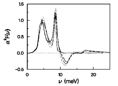
FIG. 1.: The $\alpha^{2}F(\nu)$ for Pb (solid curve) plotted vs. frequency, along with the estimates obtained from Eq. (3) with an impurity scattering rate, $1/\tau=$ (a) 1 meV (dotted), (b) 10 meV (dot-dashed), and (c) 20 meV (short-dashed-long-dashed). Note that all are qualitatively quite accurate, before they become negative at higher frequencies. Also plotted is the result (dashed curve, barely discernible from the solid curve) obtained from a full numerical inversion, as described in the text.

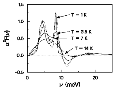
FIG. 2.: The $\alpha^{2}F(\nu)$ for Pb (solid curve) plotted vs. frequency, along with the estimates obtained from Eq. (3), using $1/\tau=10$ meV, calculated at (a) $T=1$, (b) $T=3.5$, (c) $T=7$, and (d) $T=14$ K. As the temperature is raised, the fine details are lost, but the overall energy scale remains.

of finite temperature, especially since we are examining a normal state property, and the normal state is often inaccessible at low temperatures (because of superconductivity, for example). In Fig. 2 we show the result of applying Eq. (3) to the conductivity for Pb calculated at a series of finite temperatures. The result illustrates that at sufficiently high temperature the structure is lost, although the qualitatively correct result remains: that structure in the conductivity is due to inelastic scattering in the phonon region (in the case of Pb). This procedure works fairly well, even though Eq. (3) does not even follow in the weak coupling limit at finite temperature. With these limitations in mind, we proceed for the remainder of this paper using the explicit equation (3).

We begin by using the reflectance data at 25 K for K₃C₆₀ taken by Degiorgi et al. [12]. We have performed our own Kramers-Kronig analysis on this data, to extract the complex conductivity. We should caution the reader that this procedure requires low frequency and high frequency extrapolations. Our results are essentially insensitive to the form of the high frequency extrapolation. The standard procedure for the low frequency regime is to use the Hagen-Rubens form for the reflectance [18]; however, we have used the full Drude form, since second derivatives of the conductivity are required, and hence the result may be sensitive to these approximations. We find (see below) that the low frequency result in particular is indeed sensitive to our choice of low frequency extrapolation.

To proceed with a low frequency Drude extrapolation, two parameters are required, the dc resistivity (as in the Hagen-Rubens form), and an effective electron scattering rate, which we take to be independent of frequency for low frequencies. Once these are chosen (by matching the reflectance with the experimental result at some low frequency), the frequency-dependent phase can by determined by a Kramers-Kronig integral [18]. From these follow all the optical properties of the solid, in particular the real and imaginary parts of the conductivity. Equation (3) then provides us with an estimate for $\alpha^{2}F(\nu)$. The result is plotted in Fig. 3, along with the neutron scattering data from [8]. We note several features in the figure. First, there are indeed high frequency negative regions, which our experience with Pb teaches us to ignore. Second, there is a prominent low frequency negative region (near 20 meV) for which we have no explanation, except that perhaps the low frequency extrapolation may be in error. Also note the very low frequency peak at about 5 meV, which is actually in agreement with the neutron data. On the other hand, an analysis using the Hagen-Rubens low frequency form (which is less accurate than the Drude form) leads to essentially the same result minus the low frequency peak. Hence, we cannot say for sure that this peak (attributed to librons) is coupled to the electrons. The negative region just above the libron peak persists regardless of the method of low frequency extrapolation; aside from the point noted above, it could be due to varying electron density of states effects [19], for example. We proceed, assuming the problem can be resolved by including such corrections, and discard the negative pieces in Fig. 3 for the remainder of the paper.

If we ignore the negative pieces of $\alpha^{2}F(\nu)$ the qualitative agreement with the neutron scattering data (plotted with a dashed curve [8] ) is striking. Not only is the energy scale correct, but peaks line up fairly well, suggesting that the coupling is more or less energy independent. It is difficult to assess whether contributions are truly coming from the higher energy region, as the neutron scattering data ends around 200 mev.

In any event, we can think of the $\alpha^{2}F(\nu)$ in Fig. 3 as an ”educated guess” and now proceed to calculate the expected reflectance. One might first try to fit the data by selecting a suitable plasma frequency and frequency-independent (impurity) scattering rate, so that the conductivity is Drude-like. Such an attempt fails, and it is clear that inelastic scattering is required. We use Fig. 3 without adjustment and vary (by hand) the plasma frequency and impurity scattering rate to obtain reasonable agreement with the measured reflectance. The result is plotted in Fig. 4. While significant changes in $\alpha^{2}F(\nu)$

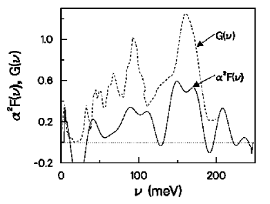
FIG. 3.: The $\alpha^{2}F(\nu)$ for K₃C₆₀ (solid curve) extracted from the reflectance data of Degiorgi et al. [12], using Eq. (3). For purposes of analysis we have omitted the negative parts (see text). Also shown are the neutron scattering results from Ref. [8] (dashed curve). Clearly the energy scale in $\alpha^{2}F(\nu)$ matches that of the phonons, and some of the peaks even line up correctly.

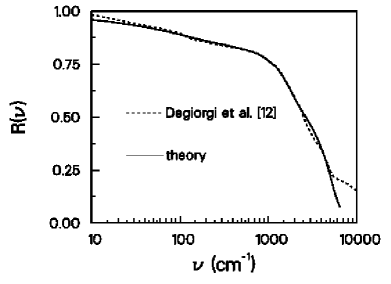
FIG. 4.: The reflectance calculated using the spectral function from Fig. 3 (solid curve) along with the drude parameters $\omega_{P}=6000$ cm^-1 and $1/\tau=95$ meV. The reflectance data of Degiorgi et al. [12] (dashed curve) are also shown.

will lead to a deterioration of the agreement shown in Fig. 4, minor adjustments can be imposed which will actually improve the agreement. However, this latter fine-tuning violates the spirit of Eq. (3), which, as we learned from the exercise with Pb, provides a qualitatively correct estimate for the bosonic spectral function.

We should note that we obtain as fitted parameters the result $\omega_{P}=6000$ cm^-1 and $1/\tau=95$ meV for the plasma frequency and impurity scattering rate, respectively. The first result is somewhat less than the result obtained via the sum rule [15], which was used in Eq. (3) ($\omega_{P}=7200$ cm^-1). We view this as a rather minor inconsistency, compared to, say, that which exists between the penetration depth-derived plasma frequency, and the one from the optical sum rule [12]. The value obtained for the impurity scattering rate is a little more disconcerting, since it is quite large. In the approach of Ref. [12] such a large scattering rate is avoided by explicitly accounting for a mid-infrared band. We could, of course, also include a mid-infrared band with extra parameters to improve the overall fit and achieve a more realistic scattering rate, but then the derived $\alpha^{2}F(\nu)$ would have more model dependence then is already implied in Eqs. (1) and (2).

Given the extracted $\alpha^{2}F(\nu)$ in Fig. 3 (without the negative components) one can ask whether or not such a spectral function can account for the superconducting properties in K₃C₆₀. To this end we have computed the Coulomb repulsion pseudopotential, $\mu^{\ast}$, given that $T_{c}=19$ K. The result is $\mu^{\ast}=0.4$ (using a cut-off, $\omega_{c}=1$ eV). The spectrum can be characterized by $\lambda=1.2$ and $\omega_{ln}=40$ meV. This gives us $T_{c}/\omega_{ln}=0.04$, which, in spite of the rather large value of $\lambda$, represents a fairly weak coupling strength. Nonetheless, the gap ratio, $2\Delta_{0}/k_{B}T_{c}$ comes out fairly close to 4, significantly different from the BCS weak coupling result, a result which is partially due to the large value of $\mu^{\ast}$ [20]. If the low frequency peak in $\alpha^{2}F(\nu)$ at 5 meV is excluded, the results are then very BCS-like: $\lambda=0.8$, $\mu^{\ast}=0.34$, $T_{c}/\omega_{ln}\approx 0.016$, and the gap ratio is $2\Delta_{0}/k_{B}T_{c}\approx 3.6$. Either of these possibilities is strongly refuted by a gap measurement of order 5 [21], though it is difficult to discriminate between the two lower values based on far-infrared measurements. Microwave measurements may provide a discriminating probe, as discussed in [22].

In conclusion, we have described an inversion scheme to extract the source of inelastic scattering in a metal. Such a scheme has many advantages over that already utilized in tunneling, not the least of which is Eq. (3), which allows a direct estimate from optical measurements with essentially no effort. Fairly accurate experiments are required however. We applied this technique to K₃C₆₀, and have found the qualitatively correct $\alpha^{2}F(\nu)$ for this material. The coupling is sufficiently strong to explain the superconductivity in this material; in fact the $\mu^{\ast}$ required is conspicuously large, so that, as suspected by many, electron-electron correlations are strong as well. Nonetheless, the weak coupling approach presented here appears to be able to account for the main features observed in the far-infrared. K₃C₆₀ is a conventional weak coupling electron-phonon superconductor with an anomalously large Coulomb pseudopotential.

We acknowledge helpful discussions with Tom Timusk. This research was supported by the Natural Sciences and Engineering Research Council (NSERC) of Canada and by the Canadian Institute for Advanced Research (CIAR).

REFERENCES

- [1] C.C. Chen and C.M. Lieber, Science 259, 655 (1993).
- [2] A.P. Ramirez et al. Phys. Rev. Lett. 68, 1058 (1992).
- [3] M.P. Gelfand, Superconductivity Review 1, 103 (1994).
- [4] W.E. Pickett, Solid State Physics 48, 226 (1994).
- [5] C.H. Pennington and V.A. Stenger, Rev. Mod. Phys. 68, 855 (1996).
- [6] O. Gunnarsson, Rev. Mod. Phys. 69, 575 (1997).
- [7] J. Ostrick has performed some preliminary tunneling measurements on these systems (private communication).
- [8] L. Pintschovius, Rep. Prog. Phys. 57, 473 (1996).
- [9] P.B. Allen, Phys. Rev. B 3, 305 (1971).
- [10] R.R. Joyce and P.L. Richards, Phys. Rev. Letts. 24, 1007 (1970).
- [11] B. Farnworth and T. Timusk, Phys. Rev. B10, 2799 (1974); ibid B14, 5119 (1976).
- [12] L. Degiorgi, E.J. Nicol, O. Klein, G. Grüner, P. Wachter, S.-M. Huang, J. Wiley and R.B. Kaner, Phys. Rev. B49, 7012 (1994). More recent results are presented in Degiorgi et al. Nature 369, 541 (1994).
- [13] G.D. Mahan, Many-Particle Physics (Plenum Press, New York, 1981).
- [14] H. Scher, Phys. Rev. Letts. 25, 759 (1970).
- [15] R. Kubo, J. Phys. Soc. Jpn. 12, 570 (1957).
- [16] We perform the weak coupling expansion somewhat differently from Allen [9]. The denominator is kept as the unperturbed part; once the integral in the expanded portion is performed, we de-expand (as Allen does—see his Eq. (61)) but we do not attempt to extract a renormalization component which leads to his undetermined function . Our result has no unknown components.
- [17] F. Marsiglio, unpublished.
- [18] F. Wooten, Optical Properties of Solids (Academic Press, New York, 1972).
- [19] B. Mitrović and M.A. Fiorucci, Phys. Rev. B31, 2694 (1985).
- [20] C.L. Sammer and J.P. Carbotte, Phys. Rev. B48, 3375 (1993).
- [21] Z. Zhang, C. Chen and C.M. Lieber, Science 254, 1619 (1991).
- [22] F. Marsiglio, J.P. Carbotte, R. Akis, D. Achkir and M. Poirier, Phys. Rev. B50, 7203 (1994). See also F. Marsiglio and J.P. Carbotte, Aust. J. Phys. 50, xxxx (1997).