Self-organized critical random directed polymers

Abstract

We uncover a nontrivial signature of the hierarchical structure of quasi-degenerate random directed polymers (RDPs) at zero temperature in $1+1$ dimensional lattices. Using a cylindrical geometry with circumference $8\leq W\leq 512$, we study the differences in configurations taken by RDPs forced to pass through points displaced successively by one unit lattice mesh. The transition between two successive configurations (interpreted as an avalanche) defines an area $S$. The distribution of moderatly sized avalanches is found to be a power-law $P(S)\,dS\sim S^{-(1+\mu)}\,dS$. Using a hierarchical formulation based on the length scales $W^{2\over 3}$ (transverse excursion) and the distance $W^{{2\over 3}\alpha}$ between quasi-degenerate ground states (with $0<\alpha\leq 1$), we determine $\mu={2\over 5}$, in excellent agreement with numerical simulations by a transfer matrix method. This power-law is valid up to a maximum size $S_{5\over 3}\sim W^{5\over 3}$. There is another population of avalanches which, for characteristic sizes beyond $S_{5\over 3}$, obeys $P(S)\,dS\sim\exp(-(S/S_{5\over 3})^{3})\,dS$ also confirmed numerically. The first population corresponds to almost degenerate ground states, providing a direct evidence of “weak replica symmetry breaking”, while the second population is associated with different optimal states separated by the typical fluctuation $W^{2\over 3}$ of a single RDP.

PACS numbers: 02.50.Ey, 05.70.Ln, 64.60.Ht

I Introduction

Self-organized criticality (SOC) [1] describes out-of-equilibrium extended systems driven infinitely slowly which respond intermittently with avalanches or bursts of sizes distributed according to power-law distributions. A close relationship between critical phase transitions and a class of SOC systems [2, 3] has been pointed out. Member systems of this SOC class operate exactly at the critical value of an underlying critical point. A necessary condition for this to occur is that the order parameter (often akin to a flux) of a dynamical critical transition be driven infinitely slowly, thus forcing the control parameter to readjust itself dynamically around its critical value [3].

Motivated by this correspondence, we introduce a new SOC model. It can be described as an equilibrium depinning problem wherein a certain type of avalanche separates local equilibrium states. The succession of equilibrium state transitions found in our model resembles the behaviour of abelian sandpiles [4]. In the latter, each avalanche can be shown to connect two different microscopic metastable states. Furthermore, its critical state is then characterized by the complete set of these avalanche-connected metastable states. Whereas the set of coexisting metastable stables is created by the threshold rules of the sandpile automata, the many coexisting local equilibrium states appearing in our model emerge from an optimal (i.e. minimum energy) configuration in a quenched random landscape. This disorder induces the coexistence of an extremely large number of almost equivalent configurations. The resulting closeness in energy space leads to a large spread in configuration space. This turns out to produce a power-law distribution for the interconnecting avalanches.

Thus, a common property of SOC systems is that they are characterized by a large set of almost equivalent and degenerate states. This set can be generated by dynamic automata rules, disorder, frustration or other mechanisms. In addition to the introduction of a new class of SOC models, our results provide further evidence for the hierarchical structure of sets of random directed polymers (RDPs).

Our results bear an apparent strong similarity to those previously obtained for pinned charged density waves [5], driven interfaces in random media [6], and elastic manifolds on disordered substrates [7]. However, the connection between the dynamic critical phenomena obtained from a constant driving force $F$ at the depinning threshold $F_{c}$ and the nearly critical behavior obtained by a small constant velocity drive is based on an argument relating the critical behavior as $F\to F_{c}^{+}$ and $F\to F_{c}^{-}$. This predicts [5, 6, 7] a vanishing exponent for the avalanche distribution in our 1+1 dimensional case, which seemingly contradicts our result. The discrepancy stems from the fact that we do not describe the same regime; the vanishing exponent refers to the existence of large avalanches of sizes controlled by the system size (or the correlation length when off-criticality applies). This corresponds to the second of two identified avalanche regimes of our model. In contrast, the present work reveals the existence of a sub-dominant power-law distribution of avalanches stemming from the hierarchy of almost equivalent degenerate states. These states do not, however, contribute to the large scale behavior and have thus been overlooked in previous work.

The model is defined in the next section, while in Sec. III we derive our theoretical predictions for the distribution of avalanche sizes. These are compared with extensive numerical simulations in Sec. IV. Our conclusions are found in Sec. V.

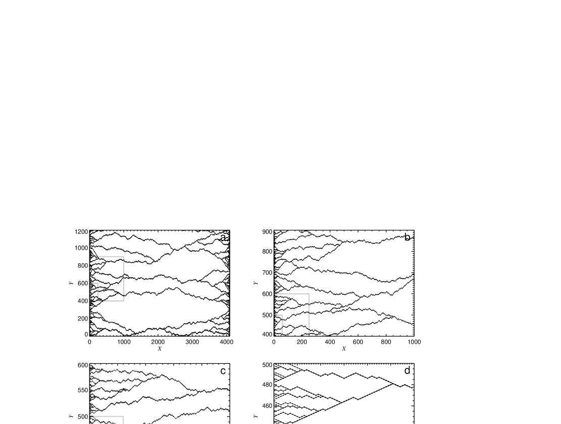
FIG. 1.: A typical set of optimal configurations for a RDP of length $W=4096$ and for $0\leq y\leq 1200$. a) global system (grey framed boxes outlines regions of succeeding plots such that the horizontal and vertical extensions of these boxes follow Eqs. (8) and (6) with $\alpha\approx 0.9$); b) magnification of the largest box in a); c) magnification of the largest box in b); d) magnification of the box in c).

II Definition of the model

Consider a RDP on a square lattice oriented at $45^{\circ}$ with respect to the $x$ axis and such that each bond carries a random number, interpreted as an energy. An arbitrary directed path (a condition of no backwards turn) along the $x$-direction and of length $W$ (in this direction) corresponds to the configuration of a RDP of $W$ bonds. In the zero temperature version we study here, the equilibrium polymer configuration is the particular directed path on this lattice which (in the presence of given boundary conditions) minimizes the sum of the $W$ bond energies along it. This simple model, with its much varied behavior, has become a valuable tool in the study of self-similar surface growths [8], interface fluctuations and depinning [9], the random stirred Burgers equation in fluid dynamics [10] and the physics of spin glasses [11].

Let us apply a field $h$ that exerts a force on one of the vertical endpoint position $y(W)$ of the polymer. This field adds a term $-h\,y(W)$ to the configurational energy of the polymer given by the sum of random bond energies along it. It is similar to a transverse electric field acting on the charged head of the polymer. If the other polymer extremity is free, the minimum energy is obtained by letting $y(W)$ go to infinity as the external field term $-h\,y(W)$ diverges to $-\infty$. This energy always dominates the configuration energy for any reasonable distribution of random bond energies. A depinning transition thus occurs for the value $h=0^{+}$ of the control parameter $h$. Mézard [12] has shown that holding the other endpoint fixed results (in the small field limit) in extremely jerky displacement of the charged head as a function of the field strength $h$. The position of the charged head is stationary for large ranges of applied field values and then changes suddenly. At the field values where these transitions (or avalanches) occur, the susceptibility attains large values. These susceptibility bursts are reportedly distributed according to a power-law [12]. This avalanche response has been attributed [12] to a “spin glass phase”, with several valleys of similar energy. It is important to realize that this avalanche behavior is not SOC as the driving is nonstationary; nothing occurs when the field stays constant and increasing the field will lead ultimately to the situation where the RDP is blocked in a fully extended configuration along the first quadrant bisectrix. This regime is similar to a mode of operation with a slow sweeping of a control parameter [13].

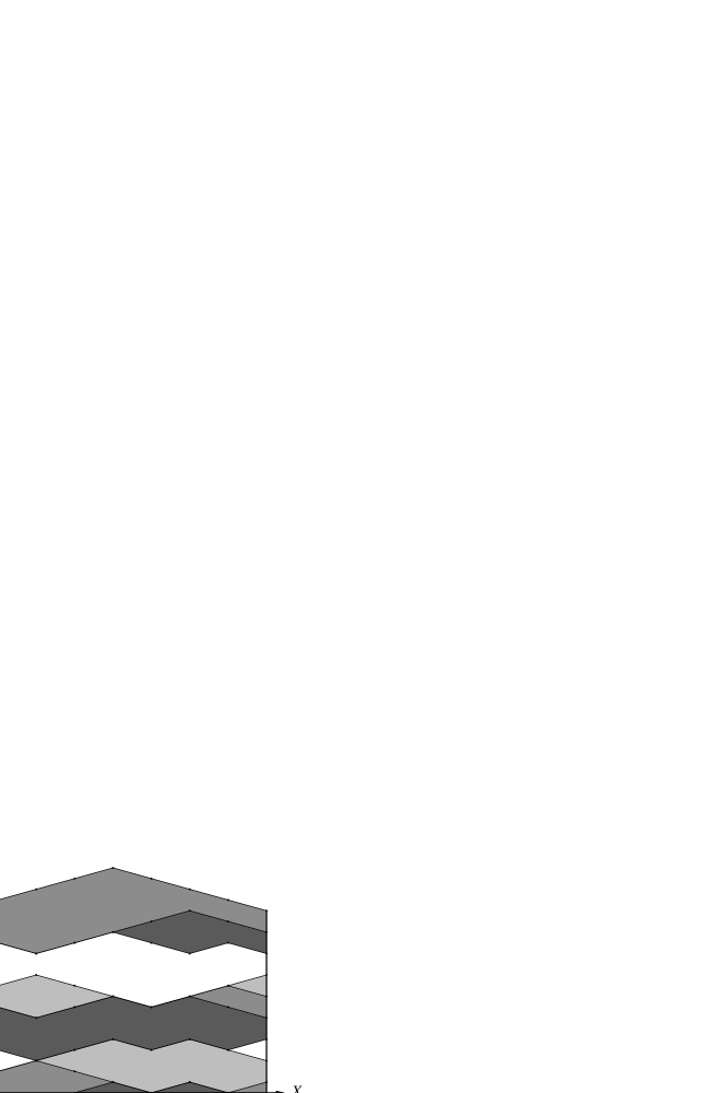
FIG. 2.: Schematic representation of optimal RDPs fixed at their two endpoints. An avalanche is defined by the area $S$ spanned by the transition from the optimal configuration at $y$ to $y+1$, i.e. $S$ is the area interior to the perimeter formed by the union of the two optimal RDP configurations at $y$ and $y+1$ and the two vertical segments $[(0,y);\,(0,y+1)]$ and $[(W,y);\,(W,y+1)]$. The successive avalanches are represented in different grey scales.

The correspondence between depinning transitions and SOC models [3] suggests, with the previous results [12], the following variant of the problem. Instead of applying a field (control parameter), we set the depinning velocity (order parameter) to an infinitesimal value [14]. This is accomplished by initially fixing the two ends of the polymer at $(x_{1}=0,y_{1}=y)$ and $(x_{2}=W,y_{2}=y)$. Since the two ordinates $y_{1}=y_{2}=y$ are equal, we could consider the case where only one endpoint is fixed while keeping the other one free, therefore making this situation correspond to a polymer on average twice as long but with both endpoints fixed. Alternatively, we may consider the polymer as wrapping itself around a cylinder of circumference $W$. The polymer is allowed to equilibrate, i.e. take the spatial configuration of minimum total bond energy. Let us now shift the vertical position of the fixed end points from $y$ to $y+1$ (where the lattice mesh is taken as unity). The polymer is again allowed to equilibrate to the spatial configuration of minimum energy. We continue in this fashion in an iterative process, which amounts to controlling the average vertical velocity of the polymer to a value so small that the time scale to move over a unit mesh is much larger than any relaxation times. This guarantees that the polymer always finds the spatial configuration of minimum bond energy. Note that the $y$ position of the polymer end points therefore functions as a clock, since no other relevant time scales are present.

Figure 1 shows a typical set of optimal configurations for a RDP of length $W=4096$ and for $0\leq y\leq L=1200$. The magnifications illustrate the self-affine structure of the RDPs and the self-similar hierarchical pattern of the local branching structure.

III Theoretical prediction of the avalanche size distribution

In this model, an avalanche at $y$ is simply the transition from the optimal configuration of a RDP with end points fixed at $y_{1}=y_{2}=y$ to the optimal configuration where the end points are now at $y_{1}=y_{2}=y+1$ (as shown in Fig. 2). We define the size of an avalanche by the area $S$ spanned by the transition from the optimal configuration at $y$ to the one at $y+1$, i.e. $S$ is the area interior to the perimeter formed by the union of the two optimal RDP configurations at $y$ and $y+1$ and the two vertical segments $[(0,y);\,(0,y+1)]$ and $[(W,y);\,(W,y+1)]$ (see Fig. 2). What do we know about the distribution of these avalanche sizes?

Clearly, the structure of the ensemble of the optimal RDPs (for all possible end point $y$ locations) uniquely determines the avalanches. For a RDP of length $W$, it is known that the typical transverse excursion $Y$ in $1+1$ dimensions scales as $Y\sim W^{\nu}$ with $\nu={2\over 3}$ (see [15] and references therein). We thus expect that there exists a class of RDP transitions with vertical lengths $Y$ of at least the order of this typical transverse excursion. The area $S$ spanned by such a transition is therefore proportional to $S\simeq WY\sim W^{5\over 3}$ (i.e. the characteristic avalanche size). The distribution of $Y$ is known to behave asymptotically as $P(Y)\sim\exp(-({Y\over W^{2\over 3}})^{3})$ [15]. Subtituting for $S\simeq WY$ in $P(Y)$ give us

$$P(S)\sim\exp(-\biggl{(}{S\over W^{5\over 3}}\biggl{)}^{3})\;,$$ (1)

for $S$ at least of the order of $W^{5\over 3}$. This constitutes our first prediction. Its validity will be tested numerically in Sec. IV.

We now derive the distribution of avalanches in the large $W$ limit for $S$ smaller than $W^{5\over 3}$. First notice that the sequence of optimal paths with fan shaped families of end points strongly resembles the ranking of paths by Zhang [16]. He found that the difference $Y$ between the endpoints of these optimal paths scale with path length $X$ as $Y\sim X^{\nu_{s}}$ with $\nu_{s}={1\over 3}$. This property is important for the understanding of our results as it suggests a hierarchical structure. We thus briefly recall its derivation.

The Bethe ansatz with the replica trick [17] provides a solution of the RDP problem in $1+1$ dimension. This shows that the RDP problem is equivalent to solving a problem of $n$ bosons in one spatial dimensions interacting with an attractive delta function potential. In this framework, imposing conditions on the endpoints of the RDP implies that the Bethe ansatz wave function must incorporate the motion of the center of mass of the $n$ bosons:

$$\Psi\sim 1/\exp(\sum_{\alpha,\beta}|x_{\alpha}-x_{\beta}|+{1\over W}\sum_{\alpha=1}^{n}x_{\alpha}^{2})\;.$$ (2)

The term ${1\over W}\sum_{\alpha=1}^{n}x_{\alpha}^{2}$ represents the kinetic and $\sum_{\alpha,\beta}|x_{\alpha}-x_{\beta}|$ the potential energy. Since $x_{\alpha}\sim W^{2\over 3}$, the kinetic energy $\sim W^{1\over 3}$. In the Bethe ansatz wave function, the potential energy must be comparable to the kinetic energy, thus $|x_{\alpha}-x_{\beta}|\sim W^{1\over 3}$, confirming that $\nu_{s}={1\over 3}$. This scaling describes the distance between degenerate ground states with so-called “weak replica symmetry breaking” [17]. Technically there is a replica symmetry breaking but the distance between the degenerate states becomes negligible compared to their intrinsic fluctuations in the thermodynamic limit.

We generalize the above observations to infer two transverse length scales $W^{2\over 3}$ and $W^{{2\over 3}\alpha}$, where $0<\alpha\leq 1$ (the case $\alpha=1$ is addressed separetely below), to describe the hierarchical structure of RDP configurations as exemplified by Fig. 1. Our results turn out to be independent of the choice of $\alpha$. Intuitively, a family of width $W^{{2\over 3}\alpha}$ consists of families of width $W^{{2\over 3}\alpha^{2}}$ each of which consists of families of smaller width and so on (down to the elemental scale of the mesh). The width, number and other properties of these embedded sets of families can be obtained from the two length scales $W^{2\over 3}$ and $W^{{2\over 3}\alpha}$ using only dimension conservation and self-similarity arguments.

1. The highest order family, that we call of order $1$, corresponds to all the locally optimal paths that are within a distance of order $W^{2\over 3}$ of a best path. The vertical width of this family of order $1$ is $w_{1}\propto W^{2\over 3}$. This family is composed of locally optimal paths that join after a distance $l_{1}\propto W$, obtained by the condition that $l_{1}^{2\over 3}\propto W^{2\over 3}$ (this condition will become nontrivial at lower levels of the hierarchy). The generic area covered by this family is $S_{1}\propto l_{1}\,w_{1}\sim W^{5\over 3}$. This is also the typical size of the largest possible avalanche as defined above and corresponds to a transition between members of this family of order $1$.

2. Within this family of order $1$, we define $N_{2}$ families of order $2$, each of which have a characteristic width $w_{2}\propto l_{1}^{{2\over 3}\alpha}\sim W^{{2\over 3}\alpha}$. It is at this point that we have used the second length scale introduced by the quasi-degenerate ground states. From the conservation of (vertical) width, we have by construction,

   $$N_{2}w_{2}=w_{1}\;,$$ (3)

   leading to $N_{2}\propto W^{{2\over 3}(1-\alpha)}$. A family of order $2$ is by itself composed of locally optimal paths that join after a distance $l_{2}\propto W^{\alpha}$, obtained by the self-consistent condition that

   $$w_{2}\propto l_{2}^{2\over 3}\;.$$ (4)

   As a consequence, the generic area, i.e. the largest possible avalanche, covered by this family of order $2$ (intra member transitions) is $S_{2}\propto l_{2}~{}w_{2}\sim W^{\alpha}\times W^{{2\over 3}\alpha}=W^{{5\over 3}\alpha}$.

3. We infer that the relevant quantities of the $n$-th order family only depends on the associated ones in the family of order $n-1$. This leads us to a recursive scheme for the calculation of the above introduced entities. In what follows we will formally define the simplest version of the iterative system of equations and state its solutions.

Within each of the families of order $n$, we define $N_{n+1}$ families of order $n+1$, each of which have a characteristic (vertical) width $w_{n+1}$. From the conservation of width, we have by construction,

$$N_{n+1}w_{n+1}=w_{n}\;.$$ (5)

The characteristic width $w_{n+1}$ relates the generic distance $l_{n}$ after which locally optimal paths (within a family of order $n$) typically join. It obeys

$$w_{n+1}=al_{n}^{{2\over 3}\alpha}\;.$$ (6)

But the self-consistency condition relates $w_{n+1}$ to $l_{n+1}$

$$w_{n+1}=Bl_{n+1}^{2\over 3}\;.$$ (7)

We are thus led to the direct recursion

$$l_{n+1}=Al_{n}^{\alpha}\;.$$ (8)

The typical area covered by an avalanche among the families of order $n+1$, is

$$S_{n+1}=Cl_{n+1}w_{n+1}\;.$$ (9)

Here $A$, $a$, $B$, and $C$ are (real valued) constants. Since $l_{1}\propto W$, we also have an initial condition for the recursion. This is generalized as

$$l_{1}=f(W)\;.$$ (10)

Finally, we have for the total number of families ${\cal N}_{n+1}$ up to and including order $n+1$,

$${\cal N}_{n+1} = N_{n+1}{\cal N}_{n}\;,$$ (11)

$${\cal N}_{1} = 1\;.$$ (12)

We find from Eqs. (8) and (10)

$$l_{n}=A^{1\over 1-\alpha}2\,\biggl{(}{f(W)\over A^{\alpha\over 1-\alpha}}\biggl{)}^{\alpha^{n-1}}\quad\mbox{for}\quad n\geq 1\;,$$ (13)

and from Eq. (7) that

$$w_{n}=BA^{2\over 3(1-\alpha)}\,\biggl{(}{f(W)\over A^{\alpha\over 1-\alpha}}\biggl{)}^{{2\over 3}\alpha^{n-1}}\;.$$ (14)

Together with Eq. (5) we then get,

$$N_{n+1}=\biggl{(}{f(W)\over A^{\alpha\over 1-\alpha}}\biggl{)}^{{2\over 3}(1-\alpha)\alpha^{n-1}}\;,$$ (15)

and from Eq. (9),

$$S_{n}=C~{}B~{}^{5\over 3(1-\alpha)}\,\biggl{(}{f(W)\over A^{\alpha\over 1-\alpha}}\biggl{)}^{{5\over 3}\alpha^{n-1}}\;.$$ (16)

The latter expression is conveniently turned into

$$\alpha^{n-1}={3\over 5}\ln\biggl{(}{S_{n}\over{CBA^{5\over 3(1-\alpha)}}}\biggl{)}/\ln\biggl{(}{f(W)\over A^{\alpha\over 1-\alpha}}\biggl{)}\;.$$ (17)

For the cumulative number of families to order $n$, i.e. Eqs. (11) and (12), we get with Eq. (15)

$${\cal N}_{n}=\biggl{(}{f(W)\over A^{\alpha\over 1-\alpha}}\biggl{)}^{{2\over 3}{(1-\alpha^{n-1})}}\;,$$ (18)

which with Eq. (17) results in a direct $S_{n}$ and $W$ dependence,

$${\cal N}_{n}=(CB)^{2\over 5}f(W)^{2\over 3}/S_{n}^{2\over 5}\;.$$ (19)

This reasoning, based on the hierarchical model, gives us the number of avalanches of specific sizes. To get the probability density distribution, we have to divide this number by the interval width from $S_{n}$ to $S_{n+1}$ which is simply proportional to $S_{n}$ up to a correction of order $S_{n}^{\alpha-1}$ as seen from Eq. (16). Gathering all the pieces and assuming that $f(W)\propto W$ leads us to the following prediction for the distribution of avalanche sizes

$$P(S)\,dS\propto{W^{2\over 3}\over S^{1+\mu}}\,dS\;,$$ (20)

with an exponent

$$\mu={2\over 5}\;.$$ (21)

The power law in Eq. (20) describes the distribution of avalanche sizes $1\leq S\leq S_{5\over 3}$ (we define $S_{5\over 3}\propto W^{5\over 3}$) in the limit $W\to\infty$. This upper scale $S_{5\over 3}$ corresponds to the maximum typical sizes of the avalanches of order $1$ in the hierarchy. Notice that the prediction of Eq. (21) is independent of the value $0<\alpha<1$ and is thus robust with respect to the detailed structure of the hierarchy.

A similar hierarchical structure can also be constructed for $\alpha=1$. In this case, it is postulated that $w_{n+1}=w_{n}/\lambda$, where $\lambda>1$ is the constant reduction factor from one level of the hierarchy to the next. While keeping Eq. (5), this leads to $l_{n+1}=l_{n}/\lambda^{3\over 2}$ and thus to $S_{n+1}=S_{n}/\lambda^{5\over 2}$ using Eq. (9). The total number of families of order $n$ is now simply proportional to $\lambda^{n}$. Solving as a function of $S_{n}$, we retrieve exactly expression (20) for the distribution of avalanche sizes.

This derivation is simpler because the hierarchical structure is exactly self-similar, with the same scaling ratio $\lambda$ throughout. This is in contrast to the case $\alpha<1$ for which $\lambda\propto w^{{2\over 3}\alpha^{n-1}(1-\alpha)}$ decreases with increasing family order. This derivation for $\alpha=1$ and $\lambda>1$ clarifies the origin of the exponent $\mu={2/5}$ stemming simply from ${1/\mu}=1+{3/2}$, i.e. from the fundamental self-affine structure of the RDP with transverse excursion exponent ${2/3}$.

We thus stress that the prediction of Eqs. (20) and (21) is very general and independent of the specific hierarchical structure of the sub-dominant quasi-degenerate ground states. Note that the power-law distribution given by Eq. (20) for the spanned surfaces is associated with two other power-laws, namely that for the distribution of typical transverse deviations $w$ and that for the distribution of typical longitudinal deviations $l$. This stems from $S\sim w\,l$ and $w\sim l^{2/3}$, leading to

$$P(w)\,dw\sim{dw\over w^{1+1}}\quad\mbox{and}\quad P(l)\,dl\sim{dl\over l^{1+2/3}}\;.$$ (22)

As mentioned in Sec. I, our finding seem to be in disagreement with the predicted value (equal to zero) for the avalanche size distribution in $1+1$ dimensions [5, 6, 7]. However, the avalanche regime of interest to us is different from that previously investigated. Our regim consists of small and intermediate avalanches of sizes up to $S_{5\over 3}$, whereas the regime which contains avalanches larger than $S_{5\over 3}$ yields a size distribution with a vanishing exponent. The present work proposes a sub-dominant power-law distribution of avalanches which originates in a hierarchical ordering of the almost equivalent degenerate states. Previous work has addressed the tail end of the avalanche distribution and has therfore not been attentive to the presence of these states.

IV Numerical tests

The distribution of avalanche sizes $S$ has been determined numerically by using a now standard transfer matrix method [18] relying on the chain property applying to the energy $e(x_{1},y_{1};x_{2},y_{2})$ of a RDP going from $(x_{1},y_{1})$ to $(x_{2},y_{2})$:

$$e(x_{1},y_{1};x_{2},y_{2})=\min_{y^{\prime}}[e(x_{1},y_{1};x^{\prime},y^{\prime})+e(x^{\prime},y^{\prime};x_{2},y_{2})]\;.$$ (23)

Figure 3 shows the distribution of avalanche sizes obtained numerically for system widths from $W=8$ to $512$. For each width, we have calculated the RDP configurations and the corresponding avalanche areas for system lengths $3\times 10^{6}\leq L\leq 2\times 10^{8}$. These very long systems provide reliable statistical estimates. In Fig. 3, the existence of a power-law for the distribution $P(S)$ is quite apparent. The size interval over which the power-law holds increases as $S_{5\over 3}\sim W^{5/3}$. Another feature of Fig. 3 is the clear evidence of a characteristic avalanche size, corresponding to the bump of the distribution in the region of large avalanche sizes. The location of these bumps also scales as $S_{5\over 3}\sim W^{5/3}$.

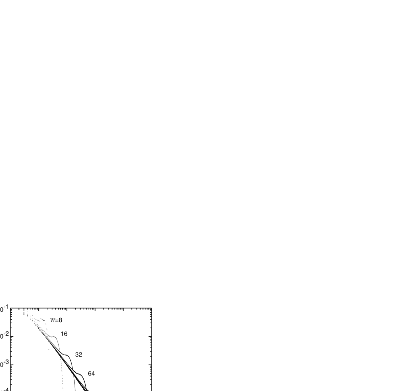
FIG. 3.: Distribution $P(S)$ of RDP avalanche sizes obtained numerically for system widths from $W=8$ to $512$ in a log-log plot. Here the system lengths $L$ are $2\times 10^{7}$ (for $W=8$), $3\times 10^{6}$ ($16$), $2\times 10^{7}$ ($32$), $10^{8}$ ($64$), $2\times 10^{8}$ ($128$), $5\times 10^{7}$ ($256$), and $9\times 10^{6}$ ($512$).

Finite size effects turn out to be very important in this problem and a careful finite size scaling analysis is appropriate. We approach this as follows.

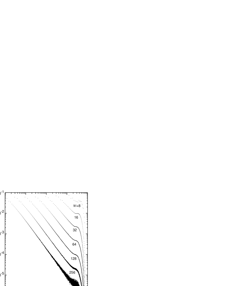
FIG. 4.: $P(S)$ as a function of the rescaled variable $S/W^{5/3}$ for $W=8$ to $512$ in a log-log plot.

FIG. 5.: The estimated $\mu$’s dependence on $W^{-2/3}$. These $\mu$ values are the result of a linear fit of $1/S^{1+\mu}$ to the linear portions in Fig. 4. The high, low, and midpoint estimates are indicated by $\bigtriangledown$, $\bigtriangleup$, and $\bullet$ respectively. The straight line is the least squares fit to the midpoint values with the five largest system widths ($W=32$, $64$, $128$, $256$, $512$). This line has been extended to the $W\to\infty$ limit.

For each system size, we determine the exponent $\mu(W)$ which best fits the numerical distribution. To demonstrate the quality of the fit, we replot Fig. 3 by showing in Fig. 4 the function $P(S)$ as a function of the rescaled variable $S/W^{5\over 3}$. For each size $W$, a different exponent $\mu(W)$ is found. The dependence of $\mu(W)$ as a function of $W^{-{2\over 3}}$ is shown in Fig. 5. We find a very good fit (“least squares”) with the finite size equation

$$\mu(W)=\mu_{\infty}-{c\over W^{2\over 3}}\;,$$ (24)

where $c=2.90$ is a constant and $\mu_{\infty}=0.40$. This is in excellent agreement with the prediction $2/5$. An apparent power-law dependence of the exponent $\mu(W)$ on $W$ as in Eq. (24) could result from fluctuations in the value of $\alpha$ within each level and accross the different levels of the hierarchy.

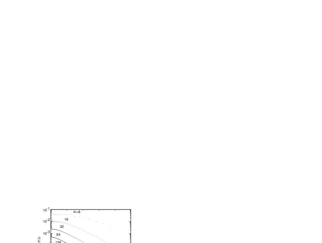
FIG. 6.: $P(s)$ for the different system sizes as a function of the rescaled variable $S^{3}/W^{5}$ in a semilog plot.

Finally, in Fig. 6 we represent $P(s)$ for the different system sizes as a function of the rescaled variable $S^{3}/W^{5}$. This choice of variables is intended to test the prediction of Eq. (1). We observe a rather convincing tendency for the plot to converge to a straight line for large system sizes.

V Conclusion

We have proposed a novel quasi-statically driven model that exhibits responses similar to those of SOC models. This model of a succession of optimal RDP configurations exhibits a power-law distribution of the area swept by a polymer between two successive optimal configurations (defined as an avalanche).

Based on the existence of two fundamental scales $W^{2\over 3}$ and $W^{{2\over 3}\alpha}$ ($0<\alpha\leq 1$) for the transverse fluctuations of a RDP of length $W$, we have constructed a hierarchical representation of the set of quasi-degenerate optimal configurations. This hierarchy allow us to calculate explicitely the exponent of the avalanche distribution.

Our numerical analysis confirm the existence of two distinct populations of avalanches. One of these populations consists of “small” avalanches that are distributed according to a power law with an upper cutoff controlled by the typical transverse length scale $W^{2\over 3}$. The other population comprises the “large” avalanches beyond this typical transverse excursion $W^{2\over 3}$.

REFERENCES

- [1] P. Bak, C. Tang, K. Wiesenfeld, Phys. Rev. A 38, 364 (1988).
- [2] C. Tang and P. Bak, Phys. Rev. Lett. 60, 2347 (1988).
- [3] D. Sornette, A. Johansen, and I. Dornic, J. Phys. I 5 , 325 (1995); D. Sornette and I. Dornic, Phys. Rev. E 54, 3334 (1996).
- [4] D. Dhar and R. Ramaswamy, Phys. Rev. Lett. 63, 1659 (1989); D. Dhar, Phys. Rev. Lett. 64, 1613 (1990).
- [5] O. Narayan and A. A. Middleton, Phys. Rev. B 49, 244 (1994).
- [6] O. Narayan and D.S. Fisher, Phys. Rev. B 48, 7030 (1993).
- [7] D. Cule and T. Hwa, preprint cond-mat/9709224
- [8] M. Kardar, G. Parisi, and Y.-C. Zhang, Phys. Rev. Lett. 56, 889 (1986).
- [9] D. A. Huse and C. L. Henley, Phys. Rev. Lett. 54, 2708 (1985).
- [10] M. Kardar, Nucl. Phys. B 290, 582 (1987).
- [11] K. Binder and A. P. Young, Rev. Mod. Phys. 58, 801 (1986); M. Mézard, G. Parisi, and M. A. Virasoro, Spin glass theory and beyond (World Scientific, Singapore, 1987).
- [12] M. Mézard, J. Phys. I 51, 1831 (1990).
- [13] D. Sornette, J. Phys. I 4, 209 (1994).
- [14] Usually, the depinning velocity would be controlled by friction and relaxation effects not discussed here; it turns out that these ingredients which are essential for describing the dynamical regime are not necessary in the SOC regime where one controls the velocity to an infinitesimal value, since this ensures that the problem consists of a succession of (at least locally) equilibrium problems.
- [15] T. Halpin-Healy, Y.-C. Zhang, Phys. Rep. 254, 215 (1995).
- [16] Y.-C. Zhang, Phys. Rev. Lett. 59, 2125 (1987).
- [17] G. Parisi, J. Physique (Paris) 51, 1595 (1990).
- [18] B. Derrida and J. Vannimenus, Phys. Rev. B 27, 4401 (1983); M. Kardar and Y.-C. Zhang, Phys. Rev. Lett. 58, 2087, (1987).