Negative superfluid densities in superconducting films in a parallel magnetic field

Abstract

In this paper we develop a theory of mesoscopic fluctuations in disordered thin superconducting films in a parallel magnetic field. At zero temperature and sufficiently strong magnetic field the system undergoes a phase transition into a state characterized by a superfluid density, which is random in sign. Consequently, in this region, random supercurrents are spontaneously created in the ground state of the system, and it belongs to the same universality class as the two dimensional $XY$ spin glass with a random sign of the exchange interaction.

Recent experiments on thin superconducting films in parallel magnetic field ^[1] have rekindled interest in this field. If the thickness of the films is small enough, the orbital effect of the magnetic field can be neglected and the suppression of superconductivity in the film is due to the Zeeman effect ^[2-4]. It has been observed that the resistance of such films at low temperatures and high enough magnetic fields exhibits very slow relaxation in time^[1]. This behavior is characteristic for spin and superconducting glasses. Below we discuss a possibility that mesoscopic fluctuations of superconducting parameters in disordered films account for such a behavior. Usually, in the limit where the electron elastic mean free path $l$ exceeds the Fermi wave length $\hbar/k_{F}$, mesoscopic fluctuations of various physical parameters of superconductors are smaller than their averages^[5-8]. Thus, they hardly affect macroscopic observable quantities. However, there are situations where mesoscopic fluctuations determine macroscopic properties of superconducting samples. One example is a superconductor in a magnetic field close to the upper critical field $H_{c2}$, where the magnetic field dependence of the superconducting critical temperature is determined by the mesoscopic fluctuations^[9]. In this paper we consider the case, where the magnetic field is parallel to the thin superconducting film and the main contribution to the suppression of superconductivity by the magnetic filed is due to Zeeman splitting of electron spin energy levels. We will show that at low temperatures $T$ and high enough magnetic fields $H$, parallel to the film, the system exhibits a transition into a state where local superfluid density $N_{s}(\vec{r})$ (which is the ratio between the supercurrent density $\vec{J_{s}}$ and the superfluid velocity $\vec{V_{s}}$) has random sign. In this case the system belongs to the same universality class as the two-dimensional $XY$ spin glass model. The idea that the superfluid density can be negative has a long history ^[5-7,10-13]. However, in the absence of magnetic fields and at zero temperature in slightly disordered superconductors ($\xi_{0}\gg l\gg{\hbar}/{k_{F}}$) the variance of the superfluid density, averaged over the superconducting coherence length $\xi_{0}=\sqrt{{D}/{\Delta_{0}}}$, turns out to be much smaller than its average^[5-8] $\langle(\delta N_{s})^{2}\rangle=G^{-2}(\langle N_{s}\rangle)^{2}\ll(\langle N_{s}\rangle)^{2}$, where $\delta N_{s}=N_{s}-\langle N_{s}\rangle$, $G$ is the dimensionless conductance of the normal metal film, in units of ${e^{2}}/{\hbar}$. Here $D={v_{F}l}/{3}$ is the diffusion coefficient, $\Delta_{0}$ is the value of the order parameter at $T,H=0$; $v_{F}$ is the Fermi velocity, and the brackets $\langle\rangle$ denote averaging over realizations of random potential. This means, that as long as $k_{F}l\gg\hbar$, the regions where the superfluid density is negative are rare and do not contribute significantly to macroscopic properties of superconductors. The situation in the presence of a magnetic field parallel to the film is different, because the average superfluid density decays with $H$ faster than its variance. Hence, at high enough magnetic field the amplitude of the mesoscopic fluctuations of $N_{s}(\vec{r})$ becomes larger than the average, and the respective probabilities of having positive and negative signs of $N_{s}(\vec{r})$ are of the same order even at $k_{F}l\gg 1$.

A theory of magnetic field induced phase transition, which does not take into account mesoscopic fluctuations predicts ^[2,14,15] that at low temperatures the superconductor-normal metal transition is of first or second order depending on whether the parameter $\Delta_{0}\tau_{so}$ is larger or smaller than unity, respectively. Here $\tau_{so}$ is the spin-orbit relaxation time.

Let us start with the case where $\Delta_{0}\tau_{so}\ll 1$. At $T=0$ and within an approximation which neglects mesoscopic effects, the value of the critical magnetic field $H^{0}_{c}$ is the result of the competition between the average superconducting condensation energy density $\langle E_{c}\rangle\sim\nu_{0}\Delta_{0}^{2}$ and the polarization energy of the electron gas in the magnetic field. Here $\nu_{0}$ is the average density of states in the metal on the Fermi surface. The average spin polarization energy density of nonsuperconducting electron gas is of order of $\langle E_{p}(0)\rangle\sim\nu_{0}(\mu_{B}H)^{2}$. Its relative change in the superconducting state is of order of $\langle E_{p}(0)\rangle-\langle E_{p}(\Delta)\rangle\sim\frac{3}{4}\pi\Delta_{0}\tau_{so}\langle E_{p}(0)\rangle\ll\langle E_{p}(0)\rangle$^[16-18]. As a result we get an expression for the critical magnetic field $H^{0}_{c}=H_{cc}(\Delta_{0}\tau_{so})^{-\frac{1}{2}}\gg H_{cc}$. Here $H_{cc}={\Delta_{0}}/{\mu_{B}}$ is the Chandrasekar-Clogston critical magnetic field of the superconductor-normal metal transition for $\Delta_{0}\tau_{so}\rightarrow\infty$ and $\mu_{B}$ is the Bohr magneton.

Now let us consider the mesoscopic fluctuations of the quantities, discussed above, in a volume whose size is of the order of the coherence length $\xi_{0}$. The amplitude of mesoscopic fluctuations of the polarization energy is of order of ^[19] $\sqrt{\langle(\delta E_{p})^{2}\rangle}\sim G^{-1}(\Delta_{0}\tau_{so})\langle E_{p}(0)\rangle$, while its $\Delta$-dependent part is of the order of

$$\frac{\sqrt{\langle(\delta E_{p}(\Delta(H))-\delta E_{p}(\Delta=0))^{2}\rangle}}{\sqrt{(\langle\delta E_{p}(0)\rangle^{2}}}\sim\left(\frac{\Delta(H)}{\Delta_{0}}\right)^{2}.$$ (1)

Here $\langle\Delta(H)\rangle=\Delta_{0}\sqrt{(H^{0}_{c}-H)/H^{0}_{c}}$ is the average superconducting order parameter. Since both the polarization energy and the condensation energy are fluctuating quantities, $\Delta(\vec{r})$ should also be spatially fluctuating. Let us consider a domain of size $L_{D}\gg\xi_{0}$ where the value of $\Delta(\vec{r})$ differs from its bulk value by a factor of order of unity. An estimate for the energy of such a domain consists of three terms, namely

$$\frac{\delta E(\Delta)}{\nu_{0}\Delta(H)^{2}dL_{D}^{2}}\sim(C_{1}\frac{1}{G}\frac{\xi_{0}}{L_{D}}+C_{2}\frac{H_{c}^{0}-H}{H^{0}_{c}}+C_{3}\frac{\xi_{0}^{2}}{L_{D}^{2}})$$ (2)

where $d$ is the thickness of the film and $C_{1},C_{2},C_{3}$ are factors of order of unity. The first term in Eq.2 corresponds to the $\Delta$-dependence of mesoscopic fluctuations of polarization energy and has a random sign. When estimating this term we have taken into account that domains of size $\xi_{0}$ make independent random sign contributions into Eq.2. The second and third term are the average condensation energy and surface (gradient) energy of the domain, respectively. It follows from Eq.2 that if $L_{D}\sim\xi(H)=\xi_{0}\sqrt{{H_{c}^{0}}/{|H-H_{c}^{0}|}}$ that there is an interval of magnetic fields near the critical one $H_{c}^{0}-H\sim H^{0}_{c}/G^{2}$, where the first term is larger than the second and the third ones. It means that, in this case the spatial distribution of $\Delta(\vec{r})$ is highly inhomogeneous and the amplitude of the spatial fluctuations of $\Delta(\vec{r})$ is of order of its average, while the characteristic size of the domains is of order of $L_{D}\sim\xi(H=H_{c}^{0}(1-1/{G^{2}}))\sim\xi_{0}G$. Superfluid density in this region has a random sign as well. To see this, one should consider states with finite superfluid velocity $\vec{V}_{s}=(\nabla\chi+{2e}/{c}\vec{A})/m$, where $\chi(\vec{r})$ is the phase of the order parameter, $\vec{A}(\vec{r})$ is the vector potential of a magnetic field perpendicular to the film and $m$ is the electron mass. If $\vec{V}_{s}(\vec{r})$ is of the order of the critical velocity, all three terms in Eq.2 are modified by factors of order of unity when compared with the case $\vec{V}_{s}=0$. The second and the third term in Eq.2 decrease with $\vec{V}_{s}$, while the first term is changed in a random direction. This means that at high enough magnetic fields, states with nonvanishing value of $\vec{V}_{s}(\vec{r})$ have lower energy than the states with $\vec{V}_{s}=0$, and that the system is unstable with respect to the creation of supercurrents of random directions. In this estimate we neglected the energy of the magnetic field associated with $\vec{V}_{s}(\vec{r})$. Since at each point of the system the possible energy gain associated with finite value of $\vec{V}_{s}(\vec{r})$ is independent of the direction of $\vec{V}_{s}$, the ground state of the system is highly degenerate and belongs to the same universality class as $XY$ spin glass with random sign of exchange interaction.

It is important to mention that even in the case of small magnetic fields in the presence of spin orbit scattering the time reversal symmetry is broken and the electron wave functions are complex. These currents flowing in the random directions exist even in normal metals. By evaluating the diagrams shown in Fig.2a, we derive the correlation function of the current density in normal metals($|\vec{r}-\vec{r^{\prime}}|\gg{\hbar}/{k_{F}}$),

$$\langle J_{i}(\vec{r})J_{j}(\vec{r}^{\prime})\rangle\approx\delta_{ij}\frac{e^{2}}{\hbar^{4}d^{2}}\tau\tau_{so}(\mu_{B}H)^{4}\delta(\vec{r}-\vec{r^{\prime}}).$$ (3)

Here $\tau={l}/{v_{F}}$ is the elastic mean free time and $i,j$ are coordinate indexes. It is important to note, however, that for a given configuration of the scattering potential and at a given value of the external field the spatial distribution of $\vec{J}(\vec{r})$ is a unique function. This implies that the currents described by Eq.3 do not exhibit features which can be associated with superconducting glass states.

Below, we will be interested in supercurrents much larger than those described by Eq.3. Such currents are spontaneously created at strong enough magnetic fields as a result of the instability associated with the random sign of superfluid density. Consider the Gorkov equation for $\Delta(\vec{r})$^[20],

$$\Delta(\vec{r})=g\int d\vec{r^{\prime}}K(\vec{r},\vec{r^{\prime}};H,\vec{A}(\vec{r}),\{\Delta(\vec{r})\})\Delta(\vec{r^{\prime}}),$$ (4)

where $K(\vec{r},\vec{r^{\prime}};H,\vec{A}(\vec{r}),\{\Delta(\vec{r})\})=kT\sum_{\epsilon}G^{\alpha\beta}_{\epsilon}(\vec{r},\vec{r^{\prime}};H,\vec{A}(\vec{r}),\{\Delta(\vec{r})\})\sigma^{x}_{\beta\mu}\tilde{G}^{\mu\nu}_{-\epsilon}(\vec{r},\vec{r^{\prime}};H,\vec{A}(\vec{r}),0)\\ \sigma^{x}_{\nu\alpha}$; $G^{\alpha\beta}_{\epsilon}(\vec{r},\vec{r}^{\prime};H,\vec{A}(\vec{r}),\{\Delta(\vec{r})\})$ is the exact one particle Matsubara Green function, $\alpha$,$\beta$, $\nu$, $\mu$ are spin indexes, $\sigma^{x}_{\alpha\beta}$ is the Pauli matrix and $\epsilon=(2n+1)\pi kT$ is the Matsubara frequency. $g$ is the dimensionless interaction constant. Both $\Delta(\vec{r})$ and $K(\vec{r},\vec{r^{\prime}})$ in Eq.4 are random functions of realizations of scattering potential in the sample. Averaging Eq.4 over realizations of the random potential and using the approximation $\langle\Delta(\vec{r})K(\vec{r},\vec{r^{\prime}})\rangle=\langle\Delta(\vec{r};H)\rangle\langle K(\vec{r},\vec{r^{\prime}},H)\rangle$ we get the above mentioned expression for $H^{0}_{c}$. In the case of strong magnetic fields, when $\Delta(\vec{r};H)\ll\Delta_{0}$, we can expand Eq.4 in terms of $\Delta(\vec{r})$. Since $\Delta(\vec{r})$ varies slowly over distances of the order of $\xi_{0}$, while $\langle K(\vec{r},\vec{r^{\prime}})\rangle$ decays exponentially for $|\vec{r}-\vec{r^{\prime}}|\gg\xi_{0}$, we can also make the gradient expansion of Eq.4. As a result we get from Eq.4

$$\left(\frac{1}{12}\xi_{0}^{2}(\nabla-\frac{2e}{c}\vec{A})^{2}+\frac{H^{0}_{c}-H}{H^{0}_{c}}\right)\Delta(\vec{r})+\int\delta K^{0}(\vec{r},\vec{r^{\prime}},H,\vec{A})\Delta(\vec{r^{\prime}})d\vec{r^{\prime}}=o(\frac{\Delta^{3}(\vec{r})}{\Delta_{0}}),$$ (5)

where $\delta K^{0}(\vec{r},\vec{r^{\prime}})=K^{0}(\vec{r},\vec{r^{\prime}})-\langle K^{0}(\vec{r},\vec{r^{\prime}})\rangle$ and $K^{0}(\vec{r},\vec{r^{\prime}})=K(\vec{r},\vec{r^{\prime}},\{\Delta(\vec{r})=0\})$. The difference between Eq.5 and the conventional Ginsburg-Landau equation is the third term in Eq.5 which accounts for mesoscopic fluctuations of the kernel $K^{0}(\vec{r},\vec{r^{\prime}})$. It is precisely this term, which at high magnetic fields leads to the random sign of superfluid density.

Employing the perturbation theory with respect to $\delta K^{0}(\vec{r},\vec{r^{\prime}})$ we get from Eq.5 an expression for the correlation function $C(\vec{r}_{1}-\vec{r}_{2})=\langle\delta\Delta(\vec{r_{1}})\delta\Delta(\vec{r_{2}})\rangle$ of the mesoscopic fluctuations of the superconducting order parameter $\delta\Delta(\vec{r};H)=\Delta(\vec{r};H)-\langle\Delta(H)\rangle$

$$C(\vec{\vec{r}_{1}}-\vec{r}_{2})\approx\frac{\Delta^{2}_{0}}{G^{2}}\left\{\begin{array}[]{cc}1-(|\vec{r_{1}}-\vec{r}_{2}|/\xi(H))^{2},&\mbox{$|\vec{r_{1}}-\vec{r}_{2}|\ll\xi(H)$};\\ \exp(-2\sqrt{3}|\vec{r_{1}}-\vec{r}_{2}|/\xi(H)),&\mbox{$|\vec{r_{1}}-\vec{r}_{2}|\gg\xi(H)$}.\end{array}\right.$$ (8)

In order to derive Eq.6 we had to calculate the correlation function $\langle\delta K^{0}(\vec{r_{1}},\vec{r_{4}})\delta K^{0}(\vec{r_{2}},\vec{r_{3}})\rangle$ using the diagrams shown in Fig.2b. It follows from Eq.6 that $\langle(\delta\Delta)^{2}\rangle$ in the two-dimensional case is almost independent of $H$, but $\langle\Delta(H)\rangle$ decreases with $H$. As a result, perturbation theory holds as long as ${\langle\Delta(H)\rangle}/{\Delta_{0}}=\sqrt{(H^{0}_{c}-H)/H^{0}_{c}}\gg G^{-1}$.

Using the expression for the supercurrent expanded in terms of $\Delta(\vec{r},H)\ll\Delta_{0}$ we have for the correlation function of the nonlocal superfluid density $N_{s}(\vec{r},\vec{r^{\prime}})$,

$$\vec{J}_{s}(\vec{r})=\frac{e^{2}}{m}\int d\vec{r^{\prime}}N_{s}(\vec{r}-\vec{r^{\prime}})\vec{V}_{s}(\vec{r^{\prime}})=\frac{e^{2}}{m}\int d\vec{r^{\prime}}(N_{s}(H)\delta(\vec{r}-\vec{r^{\prime}})+\delta N_{s}(\vec{r},\vec{r^{\prime}}))\vec{V}_{s}(\vec{r^{\prime}}),$$ (9)

$$\frac{\langle\delta N_{s}(\vec{r}_{1},\vec{r_{1}^{\prime}})\delta N_{s}(\vec{r}_{2},\vec{r_{2}^{\prime}})\rangle}{(N_{s}(H))^{2}}\sim\frac{C^{2}(\vec{r}_{1}-\vec{r}_{2})}{\langle\Delta(H)\rangle^{4}}\delta(\vec{r}_{1}-\vec{r_{1}^{\prime}})\delta(\vec{r}_{2}-\vec{r_{2}^{\prime}})+\frac{G^{-2}\xi_{0}^{4}}{|\vec{r}_{1}-\vec{r_{1}^{\prime}}|^{4}}\delta(\vec{r}_{1}-\vec{r}_{2})\delta(\vec{r_{1}^{\prime}}-\vec{r_{2}^{\prime}})$$ (10)

which is valid as long as ${\langle\Delta(H)\rangle}/{\Delta_{0}}\gg G^{-1}$ and $\xi(H)\gg|\vec{r}_{1}-\vec{r}_{2}|\gg\xi_{0}$. At $|\vec{r}_{1}-\vec{r}_{2}|\gg\xi(H)$, the correlation function in Eq.7 becomes exponentially small. Here $N_{s}(H)=N_{s}^{0}{\langle\Delta(H)\rangle^{2}}/{\Delta_{0}^{2}}$, $N_{s}^{0}=N({l}/{\xi_{0}})^{2}$ is the average superfluid density at $H=0$ and $N$ is the electron concentration in the metal. The first term of the correlation function in Eq.7 is connected to the fluctuations of the order parameter $\Delta(\vec{r})$ as shown in Fig.2c. The second term corresponds to the fluctuations of the Green functions $G_{\epsilon}(\vec{r},\vec{r}^{\prime})$ shown in Fig.2d.

Therefore if the magnetic field is close to the critical one, i.e. $|H-H_{c}^{0}|/H^{0}_{c}\sim G^{-2}$, then the amplitude of fluctuations of the superfluid density averaged over the size $\xi({H})$ becomes of order of its the average $\delta N_{s}\sim\langle N_{s}\rangle$, which means that the local value of the superfluid density, averaged over the size $\xi_{0}$, becomes of random sign. Hence the system is unstable with respect to spontaneous creation of supercurrents.

If ${|H-H^{0}_{c}|}/{H^{0}_{c}}\ll G^{-2}$, one can neglect the second term in brackets in Eq.5. Rescaling $\vec{r}\sim\vec{x}G\xi_{0},\Delta(\vec{r})\sim{\Delta_{0}}/{G}f({\vec{r}}/{G\xi_{0}})$, yields a dimensionless stochastic equation for $f(\vec{x})$

$$\nabla_{\vec{x}}^{2}f(\vec{x})+\int d\vec{x^{\prime}}\delta k(\vec{x},\vec{x^{\prime}})f(\vec{x^{\prime}})=f^{3}(\vec{x}),$$ (11)

where $\langle\delta k(\vec{x},\vec{x^{\prime}})\rangle=0$ and the correlation function $\langle\delta k(\vec{x}_{1},\vec{x^{\prime}_{1}})\delta k(\vec{x}_{2},\vec{x^{\prime}_{2}})\rangle=(\delta(\vec{x}_{1}-\vec{x^{\prime}_{1}})+G^{-2}/\{G^{-4}+(\vec{x}_{1}-\vec{x^{\prime}_{1}})^{4}\})\delta(\vec{x}_{1}-\vec{x}_{2})\delta(\vec{x^{\prime}_{1}}-\vec{x^{\prime}_{2}})$ is given by diagrams shown in Fig.2b. It follows from Eq.8 that the amplitude of fluctuation of the modulus of the order parameter $\delta\Delta(\vec{r})\sim\langle\Delta(H)\rangle\sim\Delta_{0}/G$ is of order of its average. The characteristic spatial scale of the fluctuations of $\delta\Delta(\vec{r})$ is of order of $L_{D}$. The sign of second term in Eq.8 fluctuates randomly which corresponds to the random sign of the superfluid density. The spontaneously created supercurrents in this case have random directions, their typical amplitude is of order of $J^{c}_{s}\sim N_{s}^{0}{\hbar}/{G^{3}\xi_{0}}$ and their characteristic scale of spatial correlations is also of order of $L_{D}$. The current described by Eq.3 is negligible compared with $J^{c}_{s}$ when $l\ll G^{-1}\sqrt{D\tau_{so}}$.

The fact that the sign of $N_{s}$ is random is especially clear in the case of large magnetic field, when $H-H^{0}_{c}\gg H^{0}_{c}G^{-2}$. In this case, $\Delta(\vec{r})$ is nonzero only due to existence of the rare regions, where $\delta k(\vec{x},\vec{x^{\prime}})$ is much larger than the typical value. Thus, the spatial dependence of the modulus of the order parameter has the form of superconducting domains embedded in a normal metal. These regions are connected via the Josephson effect. We can calculate the average critical current of the junctions and its variance as functions of the distance between the droplets $L_{0}$:

$$\langle J_{c}\rangle\sim G\frac{e}{\hbar}\frac{D}{L_{0}^{2}}\exp\left(-\frac{2L_{0}}{\sqrt{3}\xi(H)}\right);\langle(\delta J_{c})^{2}\rangle\sim\left(\frac{e}{\hbar}\frac{D}{L^{2}_{0}}\right)^{2}.$$ (12)

They decay with $L_{0}$ exponentially and as a power law respectively. As a result, the amplitude of the fluctuations turns out to be larger than the average, which means that $J_{c}$ has a random sign.

It is well known^[21] that at $T=0$ the long range order of the ground state of the two-dimensional $XY$ model is destroyed by an arbitrary small concentration of antiferromagnetic bonds. As we have mentioned above in the case $H\ll H^{0}_{c}$ regions, where $N_{s}(\vec{r})<0$, exist with small but finite probability. In this case, however, the properties of superconducting system are different from the $XY$ model because the supercurrents spontaneously created in these regions are screened by the Meisner effect. Thus at $H,T=0$ superconducting films should exhibit the conventional long range order. This implies that there is a critical magnetic field $H_{SG}<H_{c}^{0}$ where at $T=0$ the system has a phase transition from superconducting to the superconducting glass states $(H_{c}^{0}-H_{SG}\sim H_{c}^{0}G^{-2})$. The interval of magnetic fields where the system is in the superconducting glass state is indicated by shaded region in Fig.1.

Let us now consider the case of weak spin-orbit scattering limit $\Delta_{0}\tau_{so}\gg 1$. In this case the spin magnetization in the superconducting phase is zero. Correspondingly, the conventional theory based on the equation for average order parameter leads to the conclusion that the superconductor-normal metal transition is of first order with the critical magnetic field $H_{cc}$^[3,4]. However, the fluctuations of both magnetization energy of the normal metal and the condensation energy of the superconductor phase should lead to a nonuniform state, qualitatively similar to the case $\Delta_{0}\tau_{so}\ll 1$. The theory of this phenomenon at $\Delta_{0}\tau_{so}\gg 1$ is, however, more difficult. In this case a domains of normal phase within a bulk superconductor (or a superconducting domain in normal metal) has the surface energy of order of $dL_{D}\xi_{0}\nu_{0}\Delta_{0}^{2}$, where $L_{D}$ is the domain size. This energy is much larger than the typical energy associated with mesoscopic fluctuations in Eq.2, $dL_{D}\xi_{0}\nu_{0}(\mu_{B}H)^{2}G^{-1}$. Thus the probability of the occurrence of such domains is small as long as $G>1$. We would like to stress though, that qualitatively the case $\Delta_{0}\tau_{so}\gg 1$ is not different from the case $\Delta_{0}\tau_{so}\ll 1$ for in both cases the superconducting glass solutions survive at $T=0$ and $H>H^{0}_{c}$.

The question whether or not the quantum fluctuations of the phase of the order parameter destroy the superconducting glass state at $T=0$ and large $H$ is still open^[22-24]. At finite temperatures $T>0$, strictly speaking, the system considered above doesn’t posses a phase rigidity because of Meisner screening effect^[25]. On the other hand the two dimensional $XY$ model with random sign of exchange interaction is known not to exhibit a phase transition between the paramagnetic and the spin-glass phases^[26], again implying the absence of long range order. We acknowledge useful discussions with B.Altshuler and S.Kivelson. This work was supported by the Division of Material Sciences, U.S.National Science Foundation under Contract No.DMR-9625370 and the US-Israeli Binational Science Foundation grant no. 94-00243.

FIG. 1.: Qualitative picture of the magnetic field dependence of $\Delta(H)$ at zero temperature when $\Delta_{0}\tau_{s0}\ll 1$. The shaded region corresponds to the superconducting glass phase. $\Delta^{*}\sim\Delta_{0}/G$, $\delta H_{c}\sim H^{0}_{c}/G^{2}$.

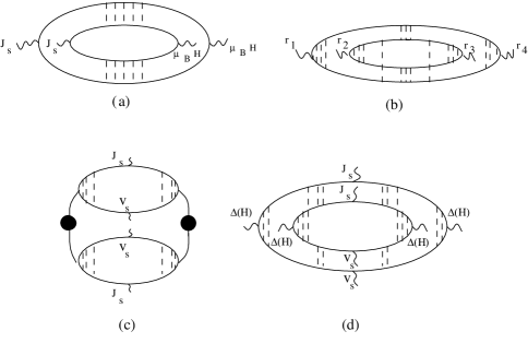
FIG. 2.: a) Diagrams representing the current correlation function Eq.3. b) Diagrams representing the correlation function $\langle\delta K^{0}(\vec{r_{1}},\vec{r_{4}})\delta K^{0}(\vec{r_{2}},\vec{r_{3}})\rangle$. c)d) Diagrams representing the correlation function of supercurrent densities $\langle\vec{J}_{s}(\vec{r})\vec{J}_{s}(\vec{r^{\prime}})\rangle$. Solid lines correspond to electron Green functions in metal and dashed lines correspond to elastic scatterings of a random potential and black dots represent the correlation function $\langle\delta\Delta(\vec{r}_{1})\delta\Delta(\vec{r}_{2})\rangle$ given by Eq. 6.

REFERENCES

• [1] Permanent Address: Physics Department, Princeton University, Princeton, NJ 08540.
• [2] W. Wu, P. W. Adams, Phys. Rev. Lett. 74, 610(1995).
• [3] A. A. Abrikosov, Fundamentals of The Theory of Metals, North-Holland, 1988.
• [4] A. M. Clogston, Phys. Rev. Lett. 9, 266(1962).
• [5] B. S. Chandrasekhar, Appl. Phys. Lett. 1, 7(1962).
• [6] B. Altshuler B. Spivak, Zh. Eksp. Teor. Fiz. 92, 609(1987) [Sov. Phys. JETP 65, 343(1987)].
• [7] B. Spivak, A. Zyuzin, Pisma Zh. Eksp. Teor. Fiz. 47, 221(1988) [Sov. Phys. JETP Lett. 47, 267(1988)].
• [8] B. Spivak, A. Zyuzin, Mesoscopic fluctuations of Current Density in Disordered Conductors, Mesoscopic Phenomena in Solids edited by B. Altshuler, P. Lee and R. Webb, Elsevier Science Publishers B. V., 1991.
• [9] C. W. J. Beenakker, Phys. Rev. Lett. 67, 3836(1991).
• [10] B. Spivak, F. Zhou, Phys. Rev. Lett. 74, 2800(1995).
• [11] A. Aronov, B. Spivak, Fiz. Tverd. Tela 17, 2806 (1975) [ Sov. Phys. Solid State 17, 1874 (1975)].
• [12] L. Bulaevski, V. Kuzzi, A. Sobianin, Pisma Zh. Eksp. Teor. Fiz. 25, 314(1977) [JETP Lett. 25, 7(1977)].
• [13] B. Spivak, S. Kivelson, Phys. Rev. B 43, 3740(1991).
• [14] S. Kivelson, B. Spivak, Phys. Rev. B 45, 10492(1990).
• [15] N. R. Werthamer, E. Helfand, P. C. Hohenberg, Phys. Rev. B 147, 295(1966).
• [16] K. Maki, Phys. Rev. B 148, 362(1966).
• [17] R. A. Ferrell, Phys. Rev. Lett. 3, 262(1959).
• [18] P. W. Anderson, Phys. Rev. Lett. 3, 325(1959).
• [19] A. A. Abrikosov, L. P. Gorkov, Sov. Phys. JETP 15, 752(1962).
• [20] H. Yoshika, Jour. Phys. Soc. Japan 63, 405(1994).
• [21] A. A. Abrikosov, L. P. Gorkov, I. E. Dzyaloshinski, Methods of Quantum Field Theory in Statistical Physics, Dover, 1975.
• [22] J. Villain, Jour. Phys. C 10, 4793(1977).
• [23] M. Fisher, Phys. Rev. Lett. 57, 885(1986).
• [24] S. Chakravarty, S. Kivelson, G. Zimanyi, B. Galperin, Phys. Rev. B 35, 7256(1987).
• [25] V.J. Emery, S.A. Kivelson, Phys. Rev. Lett. 74, 3253 (1995).
• [26] J. M. Kosterlitz, D. J. Thouless, J. Phys. C 6, 1181(1973).
• [27] B. W. Moris, S. G. Golbourne, M. A. Moore, A. J. Bray, J. Canisis, J. Phys. C 19, 1157(1986).
Refer to caption