January 1998

UT-KOMABA/98-3

cond-mat/9801307

Counting Hamiltonian cycles
on planar random lattices

Saburo Higuchi

Department of Pure and Applied Sciences,

The University of Tokyo

Komaba, Meguro, Tokyo 153-8902, Japan

Abstract

A Hamiltonian cycle of a graph is a closed path which visits each of the vertices once and only once. In this article, Hamiltonian cycles on planar random lattices are considered. The generating function for the number of Hamiltonian cycles is obtained and its singularity is studied. Relation to two-dimensional quantum gravity is discussed.

Hamiltonian cycles have often been used to model collapsed polymer globules[1]. A Hamiltonian cycle of a graph is a closed path which visits each of the vertices once and only once. The number of Hamiltonian cycles on a graph corresponds to the entropy of polymer system on it in collapsed but disordered phase. There can be no polynomial time algorithms to determine whether the number is zero or not which work for arbitrary graphs[2]. Even for regular graphs (lattices), the number of Hamiltonian cycles is not obtained exactly except for a few well-behaved cases[3, 4, 5, 6]

In the present work, I consider the problem of counting the number of Hamiltonian cycles on planar random lattices, or planar random fat graphs. I obtain the exact generating function for the number.

Let $S^{n}$ be the set of all planar trivalent fat graphs with $n$ vertices possibly with multiple edges and self-loops. Graphs that are isomorphic are identified. The set $\tilde{S}^{n}$ is the labeled version of $S^{n}$, namely, vertices of $\tilde{G}\in\tilde{S}^{n}$ are labeled as $1,\ldots,n$ and $\tilde{G}_{1},\tilde{G}_{2}\in\tilde{S}^{n}$ are considered identical only if a graph isomorphism preserves labels. The symmetric group of degree $n$ naturally acts on $\tilde{S}^{n}$ by label permutation. The stabilizer subgroup of $\tilde{G}$ is called the automorphism group $\mathrm{Aut\ }G$.

A Hamiltonian cycle of a labeled graph $\tilde{G}\in\tilde{S}^{n}$ is a directed closed path (consecutive distinct edges connected at vertices) which visits each of $n$ vertices exactly once. Hamiltonian cycles are understood as furnished with a direction and a base point. The number of Hamiltonian cycles of $\tilde{G}$ is denoted by $\mathcal{H}(G)$ because it is independent of the way of labeling. See figure 2 for an example.

The quantity I study in this work is

$$F_{n}=\sum_{G\in S^{n}}\mathcal{H}(G)\frac{1}{\#\mathrm{Aut\ }G}$$ (1)

and the generating function

$$F(p)=\sum_{n=0}^{\infty}p^{n}F_{n}.$$ (2)

It is illuminating and is useful to rewrite $F_{n}$ as the number of isomorphism classes of the pair (graph, Hamiltonian cycle):

$$F_{n}=\#(\{(\tilde{G},C^{n})|\tilde{G}\in\tilde{S}^{n},C^{n}:\text{Hamiltonian cycle on }\tilde{G}\}/\sim),$$ (3)

where $(\tilde{G}_{1},C^{n}_{1})\sim(\tilde{G}_{2},C^{n}_{2})$ if and only if $G_{1}$ and $G_{2}$ are isomorphic (forgetting the labels) and the isomorphism maps $C^{n}_{1}$ onto $C^{n}_{2}$ with the direction and the initial point preserved. Eq. (3) implies that $F_{n}$ is an integer though the definition (1) involves a fraction.

The equality (3) can be shown as follows.

$$\#\{(\tilde{G},C^{n})|\tilde{G}\in\tilde{S}^{n},C^{n}:\text{Hamiltonian cycle on }\tilde{G}\}/\sim$$

$$= \frac{1}{n!}\sum_{\tilde{G}\in\tilde{S}^{n}}\#\{C^{n}|C^{n}:\text{Hamiltonian cycle on }\tilde{G}\}$$

$$= \frac{1}{n!}\sum_{\tilde{G}\in\tilde{S}^{n}}\mathcal{H}(G)$$

$$= \frac{1}{n!}\sum_{G\in S^{n}}\frac{n!}{\#\mathrm{Aut\ }G}\mathcal{H}(G).$$ (4)

The first equality follows from the fact that there are $n!$ inequivalent labeling of $(G,C)$. In the last line, the definition of $\mathrm{Aut\ }G$ is made use of.

To compute $F(p)$, the method used in refs. [7, 8, 9] is followed. One walks along the Hamiltonian cycle in the specified direction starting from the base point and records the order of right and left turns. Then one obtains a diagram consisting of T’s as depicted in the center of figure 2. A cycle corresponds to exactly 2 out of $2^{n}$ diagrams consisting of $n$ T’s. The two are mirror images of each other.

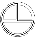
Figure 1: An example of planar trivalent fat graph $G$ with $n=4$. A Hamiltonian cycle is drawn in thick line. For this graph, $\mathcal{H}(G)=4!$ because I distinguish the directions and the base points of the cycle.

Figure 2: Two of contributing diagrams for $n=6$. The sequence of T’s in the center is obtained by walking along the Hamiltonian cycle (the thick line in the T’s). Openings in both sides should be connected by arcs. On the left hand side, there is a single possibility because $A_{2}=1$. On the right hand side, $A_{4}=2$ and the two possible patterns are drawn.

There are $\binom{n}{k}$ diagrams that have $k$ openings on the left hand side and $n-k$ on the right hand side. To reproduce the graph completely, one has to connect the $n$ openings pairwisely. There should be no connection between the right hand side and the left hand side because the cycle divides the sphere into two disks. The connection pattern should be able to be drawn on a disk faithfully, i.e. without intersection. The number of ways of contracting $k$ objects on a disk is denoted by $A_{k}$. Then one has

$$F_{n}=\sum_{k=0}^{n}\frac{1}{2}\binom{n}{k}A_{k}A_{n-k}.$$ (5)

The factor $1/2$ comes form the identification of the mirror images. There is no double count besides it. The number $A_{k}$ has been obtained by Brézin et. al. using the gaussian matrix model [10]:

$$A_{k}=\frac{1}{2\pi}\int^{2}_{-2}dx\sqrt{4-x^{2}}\quad x^{k}=\begin{cases}0&(k:\text{odd}),\\ \frac{k!}{(\frac{k}{2})!(\frac{k}{2}+1)!}&(k:\text{even}).\end{cases}$$ (6)

Plugging this into eq.(5), one has

$$F(p)= \sum_{n=0}^{\infty}p^{n}\frac{1}{2}\frac{1}{2\pi}\int^{2}_{-2}dx\sqrt{4-x^{2}}\frac{1}{2\pi}\int^{2}_{-2}dy\sqrt{4-y^{2}}(x+y)^{n}$$

$$= \frac{1}{2}\frac{1}{2\pi}\int^{2}_{-2}dx\sqrt{4-x^{2}}\frac{1}{2\pi}\int^{2}_{-2}dy\sqrt{4-y^{2}}\frac{1}{1-A(x,y;p)},$$ (7)

where

$$A(x,y;p)=px+py$$ (8)

By using

$$\frac{1}{1-px-py}=\int^{\infty}_{0}d\alpha\quad e^{(-1+p(x+y))\alpha},$$ (9)

one obtains

$$F(p)=\frac{1}{2p^{2}}\int^{\infty}_{0}d\alpha\quad\frac{e^{-\alpha}}{\alpha^{2}}(I_{1}(2p\alpha))^{2},$$ (10)

where $I_{1}$ is the modified Bessel function of the first order.

From the representation (7), it is apparent that $F(p)$ diverges at $p=1/4$. The singularity of $F(p)$ brings information of large-$n$ behavior of $F_{n}$. By studying it one can inspect the properties of large graphs. One can show that $F(p)$ has a singularity

$$F(p)=\frac{1}{16\pi p^{3}}(4p-1)^{2}\log|4p-1|+\text{regular terms}.$$ (11)

by examining (7). This result is in accord with the scaling behavior of a polymer loop with a base point on planar random surfaces in the dense phase

$$F(p)\sim(p-\tfrac{1}{4})^{2}$$ (12)

obtained in [7].

Each planar trivalent fat graph corresponds to a triangulation of a sphere under the dual transformation. Thus $F(p)$ is the partition function of two-dimensional quantum gravity with an unusual weight. Triangulations that do not admit a Hamiltonian cycle are excluded from the path integral. On the other hand, ones admitting Hamiltonian cycles are weighted by $\mathcal{H}(G)$. Eq. (11) shows that the string susceptibility exponent $\gamma_{\text{string}}$ for this system is zero. Because there is a base point on the Hamiltonian cycle, one has a local degree of freedom which gives rise to a factor proportional to the area of the surface. In this viewpoint, one should compare the value $\gamma_{\text{string}}=0$ with scaling exponent of $c=-2$ quantum gravity with a puncture operator inserted.

This system can be generalized by introducing two parameters $p_{1}$ and $p_{2}$ as

$$F(p_{1},p_{2})=\sum_{k,m=0}^{\infty}p_{1}^{k}p_{2}^{m}\sum_{G\in S^{k+m}}\frac{1}{\#\mathrm{Aut\ }G}\mathcal{H}_{k,m}(G),$$ (13)

where $\mathcal{H}_{k,m}(G)$ denotes the number of Hamiltonian cycle with $k$ right turns and $m$ left turns. Then straightforward calculation shows

$$F(p_{1},p_{2})= \frac{1}{2}\frac{1}{2\pi}\int^{2}_{-2}dx\sqrt{4-x^{2}}\frac{1}{2\pi}\int^{2}_{-2}dy\sqrt{4-y^{2}}\frac{1}{1-p_{1}x-p_{2}y}$$

$$= \frac{1}{2p_{1}p_{2}}\int^{\infty}_{0}d\alpha\frac{e^{-\alpha}}{\alpha^{2}}I_{1}(2p_{1}\alpha)I_{1}(2p_{2}\alpha)$$

$$= \frac{1}{16\pi p_{1}^{3/2}p_{2}^{3/2}}(2p_{1}+2p_{2}-1)^{2}\log|2p_{1}+2p_{2}-1|+\text{regular terms}.$$ (14)

The function $F(p_{1},p_{2})$ is not only symmetric but with a singularity described in terms of $p_{1}+p_{2}$ only. This implies that the sum is dominated by the cycles with an equal number of right and left turns. The fluctuating geometry does not change the dominance of the maximum of the factor $\binom{k+m}{k}$ at $k=m$. I comment that in (13) the integer $\frac{2}{3}\pi(k-m)$ can be considered as the holonomy [9] of the cycle if one regards the system as a quantum gravity.

This solution can be extended to planar $q$-valent fat graph. One should just replace $A(x,y;p)$ in (7) by $A(x,y;p)=p\sum_{s=0}^{q-2}x^{s}y^{q-2-s}$. One can even consider the system with

$$A(x,y;\{p_{i,j}\})=\sum_{i,j=0}^{N}p_{i,j}x^{i}y^{j}.$$ (15)

The system now describes Hamiltonian cycles on graphs consisting of $(i+j+2)$-valent vertices with various $i,j$. The weight $p_{i,j}$ corresponds to the $2\pi\times\frac{i+1}{i+j+2}$-turn on a $(i+j+2)$-valent vertex. For example, if one takes $A(x,y;p_{1},p_{2})=p_{1}x^{2}+p_{2}xy+p_{1}y^{2}$, Hamiltonian cycles with bending energy parameterized by $p_{1}/p_{2}$ are realized on a random 4-valent lattice.

When one generalizes the system as (15), the critical line of $F(\{p_{i,j}\})$ is

$$A(x,y,\{p_{i,j}\})=1.$$ (16)

Assume that there exists $q_{0}-2\in\mathbb{N}$ such that

$$p_{i,j}=0\text{\ if }i+j>q_{0}-2,$$ (17)

$$p_{i,j}\neq 0\text{\ if\ }i+j=q_{0}-2.$$ (18)

This amounts to assuming that the largest coordination number of the graph is $q_{0}$ and the cycle can turn arbitrarily on the vertex. From direct evaluation of singular part of (7) with (15), one can show that the singularity of $F(\{p_{i,j}\})$ is still of the form

$$F(\{p_{i,j}\})\sim(\delta p)^{2}\log\delta p,$$ (19)

where $\delta p$ is a function of $p_{i,j}$’s which vanishes linearly on the critical curve.

This fact can be understood as follows. Let us look at the original case (7) with (8). The range of integration of $x,y$ is the square domain $-2\leq x,y\leq 2$. The singularity occurs when the line $1-px-py=0$ touches this domain as depicted in Fig. 3. It occurs on $(x,y)=(2,2)$ assuming $p>0$. In the case (15), the critical curve is now an algebraic curve (16). It intersects the square at $(x,y)=(2,2)$ transversally. The curve can be approximated by a straight line with a slope when one is interested in critical behaviors. The slope is the only relevant parameter at the criticality.

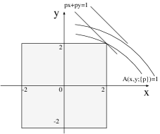
Figure 3: The shaded region is the domain of integration (7). The singularity occurs when the line $px+py=1$ touches this shaded region. For the generalized case (15), the line is replaced with an algebraic curve $1=A(x,y,\{p_{i,j}\})$ but the local situation around $(x,y)=(2,2)$ is the same as the original case.

In conclusion, I have obtained the generating function for the number of Hamiltonian cycles on planar random lattices and have considered the limit of large graphs.

I thank Mitsuhiro Kato for useful discussions. This work is supported by CREST from Japanese Science and Technology Corporation.

While this paper is being typed, a preprint by B. Eynard, E. Guitter, and C. Kristjansen has appeared [11]. It contains interesting results closely related to the present paper. Their definition of Hamiltonian cycle is slightly different from that taken here; they do not associate directions and base points to cycles.

References

- [1] J. des Cloizeaux and G. Jannik, Polymers in solution: their modelling and structure, Clarendon Press, Oxford, 1987.
- [2] M. R. Garey and D. S. Johnson, Computers and intractability — A guide to the theory of NP-completeness, W. H. Freeman, San Francisco, 1979.
- [3] P. W. Kasteleyn, Physica(Utrecht) 29 (1963) 1329.
- [4] E. H. Lieb, Phys. Rev. Lett. 18 (1967) 692.
- [5] J. Suzuki, J. Phys. Soc. Japan 57 (1988) 687.
- [6] M. Batchelor, J. Suzuki, and C. Yung, Phys. Rev. Lett. 73 (1994) 2646.
- [7] B. Duplantier and I. K. Kostov, Nucl. Phys. B340 (1990) 491.
- [8] B. Duplantier and I. K. Kostov, Phys. Rev. Lett. 61 (1988) 1433.
- [9] N. Ishibashi, Phys. Lett. B312 (1993) 411.
- [10] E. Brézin, C. Itzykson, G. Parisi, and J.-B. Zuber, Comm. Math. Phys. 59 (1978) 35.
- [11] B. Eynard, E. Guitter, and C. Kristjansen, Hamiltonian cycles on a random three-coordinate lattice, University of Durham preprint DTP-97-63, cond-mat/9801281.