Weighted Density Functionals for Ferroelectric Materials

Abstract

The weighted density approximation, its implementation and its application to ferroelectric materials is discussed. Calculations are presented for several perovskite oxides and related materials. In general the weighted density approximation is found to be superior to either the local density or generalized gradient approximation for the ground state. Electronic structures are little changed. The linear response of the weighted density approximation is calculated for the homogeneous electron gas, and found to be improved relative to the local density result, but not in full agreement with existing Monte Carlo data. It is shown that the agreement can be further improved by a simple modification. Calculations of the ferroelectric soft mode in KNbO₃ suggest that the low temperature distortion is approximately 20% smaller than indicated by existing experiments.

I Introduction

Piezoelectric, ferroelectric and related perovskites are both technologically important and physically interesting systems and, as such, have been the subject of considerable recent interest. Several groups have performed first principles calculations based on density functional theory. These calculations, primarily based on the local density approximation (LDA) have elucidated important aspects of the underlying physics of these materials as well as providing quantitative information about phonons, polarizations, crystal structure, elastic and other properties. proc97

Two of the many themes that have emerged are (1) Ferroelectric and piezoelectric properties are due to a delicate balance between large competing interactions, c92 ; c92a so very high accuracy is required for predictive calculations and (2) The lattice instabilities behind these phenomena are extraordinarily sensitive to volume. In fact, in important materials, like KNbO₃ s92 ; p93 ; p95 ; k95 ; w97 ; s95 ; s97 and BaTiO₃ c92 ; c92a ; ck90 ferroelectricity, while predicted at the experimental volume, is absent, or at least strongly suppressed, at the predicted LDA volume.

Generally excellent agreement with experimental knowledge has been obtained when calculations are performed at the experimental volume. This includes even transition temperatures, polarizations and transition temperatures proc97 . In antiferroelectric PbZrO₃, LDA calculations singh-pb at the experimental volume yielded a crystal structure that differed from existing experimental measurements. However, the LDA structure has now been confirmed by two independent neutron investigations, egami ; fujishita providing yet another demonstration of the utility of the first principles approach. On the other hand, even at the experimental volume, the LDA consistently overestimates the dielectric constant, $\varepsilon_{\infty}$. dalcorso ; resta1 ; resta2 Exploration of novel systems that are of necessity less well studied experimentally than current materials will require an ability to calculate properties independent of experimental measurements of the volume. This may also be important for determination of piezoelectric properties in materials like PbTiO₃ where the LDA gives an incorrect prediction of the strain associated with the deviation of the $c/a$ ratio from unity even with the volume constrained. ss This raises the question of whether there is a practical way of correcting the LDA errors, in order to construct a more predictive first principles approach for these materials.

The LDA errors can sometimes be trivially fixed. For example, if the experimental volume is known, the calculations may be done constrained to this volume. In some cases, e.g. KNbO₃, simple modification of the LDA functional through use of the Wigner form rather than an electron gas-like form, k95 ; w97 or the use of generalized gradient approximations (GGA) to density functional theory are sufficient to correct the volume (although the dielectric constant remains too high). However, in general these approaches do not solve the LDA problem. For example, in BaTiO₃ the GGA overcorrects the LDA volume, so that the error is as large but in the opposite direction. s95 The implication is that a more sophisticated, presumably non-local, density functional is needed to fully circumvent the problems noted above with the LDA.

The first efforts at developing practical non-local functionals date from the 1970’s when the average density approximationolle1 (ADA) and weighted density approximationolle2 ; AG ; GJL (WDA) were proposed. However, over most of the intervening period the field has been relatively dormant, in part because of the success of the simpler LDA and GGA schemes and in part because it was widely thought that such schemes could not be implemented in a computationally tractable fashion. However, at least for the WDA, computationally efficient algorithms are now known s97 ; Singh ; tet ; char and benchmark calculations have been reported. The ADA has attracted less interest.

In the cases that have been studied ground state properties of solids are generally improved over the LDA. char1 These include tests for several simple elements and compounds and KNbO₃. Significantly, this latter test showed that the WDA predicts an equilibrium volume for KNbO₃ in almost perfect agreement with experiment. s97 Unlike the GGA, which also greatly improves the equilibrium volume of KNbO₃, the WDA is a truly non-local density functional, in that the exchange correlation potential at a point r incorporates information about the charge density $n({\bf r}^{\prime})$ over a finite region of space.

Here, following a brief overview of the method, we report investigations of a range of perovskite and related oxides within the WDA. These show much improved volumes relative to either the LDA or GGA. Phonon frequencies and the ferroelectric soft mode in KNbO₃ are calculated within the WDA and compared with LDA results and experiment. An analytical expression for the linear response of the uniform electron gas in the WDA is derived.

II The Weighted Density Approximation

The WDA and the ADA are both based on the general expression for the exchange correlation energy of a general electron gas $E_{xc},$ in density functional theoryi (DFT).

$$E_{xc}=\frac{e^{2}}{2}\int\frac{n({\bf r})n({\bf r}^{\prime})}{|{\bf r-r}^{\prime}|}G({\bf r,r}^{\prime})\{n({\bf r)}\}d{\bf r}d{\bf r}^{\prime},$$ (1)

where the function $G({\bf r,r}^{\prime})$ is also a functional of the total electronic density $n{\bf(r).}$ A rigorous expression for $G$ can be derivedIEG in terms of coupling constant averaged pair correlation function:

$$G({\bf r,r}^{\prime})=\int_{0}^{1}[\bar{g}({\bf r,r}^{\prime};\lambda)\{n({\bf r)}\}-1]d\lambda.$$ (2)

Were the actual pair correlation function used instead of the coupling constant averaged one, this expression would give the interaction energy of each electron with its exchange correlation hole. The difference due to the averaging reflects the fact that kinetic energy of interacting electrons differs from that of a non-interacting system with the same density. It is this difference, also known as exchange-correlation kinetic energy, which is responsible for the high q, short wavelength behavior of the response, and is also implicated in usual underestimation of semiconducting gaps in Kohn-Sham DFT.

For the uniform gas this function, $G_{0}(|{\bf r-r}^{\prime}|,n),$ is known with high accuracyPW , but for an arbitrary inhomogeneous system, like occurs in a real density functional calculation for a solid, $G$ is not known and there is therefore no practical way to use this formula without making some approximation.

The LDA instead of Eq. (1) uses $(e^{2}/2)\int d{\bf r}d{\bf r}^{\prime}n^{2}({\bf r})G_{0}[|{\bf r-r}^{\prime}|,n({\bf r)]}/|{\bf r-r}^{\prime}|,$ so that $E_{xc}$ becomes $E_{xc}^{LDA}=\int n({\bf r})\epsilon_{xc}[n({\bf r)]}d{\bf r,}\ \ \epsilon_{xc}$ being the density of exchange-correlation energy of the uniform gas. The LDA is incorrect in both most important limits: the fully localized, i.e., a one electron system, and the fully delocalized limit, i.e., homogeneous electron gas. In the former case the LDA gives a spurious self-interaction with energy $(e^{2}/2)\int d{\bf r}d{\bf r}^{\prime}n({\bf r})n({\bf r}^{\prime})/|{\bf r-r}^{\prime}|+\int n({\bf r})\epsilon_{xc}[n({\bf r)]}d{\bf r},$ which is widely thought sic to be a key problem with the LDA. In the homogeneous limit, the LDA gives the correct exchange-correlation energy, but the changes of this energy upon small perturbations are not properly described; the second variation of $E_{xc}$ with density, i.e., the exchange-correlation part of the dielectric response, $K_{xc}({\bf r-r}^{\prime})=\delta^{2}E_{xc}/\delta n({\bf r})\delta n({\bf r}^{\prime}),$ is a delta function, which is incorrect. The Fourier transform of $K_{xc}(r)$ in LDA is independent of the wave vector. Since LDA is exact for the uniform gas, $K_{xc}^{LDA}$ corresponds to the correct $K_{xc}$ at $q=0.$ GGAs also give correct behavior at $q=0$, but become even worse than the LDA at high $q$’s.

The two nonlocal expressions for $E_{xc}$, WDA and ADA, are aimed at correcting one or the other of these two limits. The former uses the general expression (1), but instead of the actual function $G$ uses a model function, defined so that the one electron limit is honored. This begins by choosing a generic expression for $G,$ which depends on one parameter $\bar{n},$ to be defined later. In the original papers it was suggested that $G({\bf r,r}^{\prime},\bar{n})=G_{0}({\bf r,r}^{\prime},\bar{n})=\int_{0}^{1}[\bar{g}({\bf r,r}^{\prime};\lambda,\bar{n})-1]d\lambda$, where $\bar{g}$ is the averaged pair correlation function of the homogeneous electron gas. Later it was realizedGJ that other choices of $G$ may be better than $G_{0},$ and that there is no physical reason to prefer $G_{0}$ over many other choices. In the WDA $\bar{n}$ is a function of ${\bf r,}$ but differs from $n({\bf r),}$ and is chosen so that $\int G[{\bf r,r}^{\prime},\bar{n}({\bf r})]n({\bf r}^{\prime}{\bf)}d{\bf r}^{\prime}=-1.$ This assures that for a one electron system $E_{xc}$ cancels the self-interaction exactly.

Within the WDA, non-local information about the charge density is incorporated into $E_{xc}$ both through the construction of $\bar{n}$ via the sum rule, and through the non-local Coulomb integral.

We note that $G$ need not neccesarily be the actual pair correlation function of the system: although Eq.(1) has the same functional form as the WDA energy, the fact that $G^{WDA}$ is a function of an averaged density $\bar{n}$, not a functional of the true density $n({\bf r})$, means that it is possible that the best approximations for $G^{WDA}$ could be different from the physical function $G$ defined in Eq. (2) even for the uniform electron gas. However, the few reported calculations suggest that this function, while perhaps not optimal, does yield results much superior to the LDA. Besides, use of the homogeneous electron gas averaged pair correlation function has an appealing simplicity and calculations of ground state properties, below, use this ansatz. The results confirm that at least for the structural properties considered, the WDA with this choice of $G$ yields results that are uniformly superior to the LDA.

III Ground State Properties in the WDA

As mentioned, one of the basic problems with application of the LDA to ferroelectric materials is the high sensitivity of ferroelectric properties to the volume, combined with the several percent errors in predicted LDA equilibrium volumes. One of our main goals is to determine whether the WDA can repair this problem while retaining the good features of the LDA. We begin by calculating the equilibrium volumes of several cubic or near cubic oxides, namely CaO, SrO, BaO, BaTiO₃, KNbO₃ and KTaO₃. Some results for KNbO₃ were reported previously. s97 The LDA underestimates the cubic lattice parameters of these materials by 1-2%, while at least in BaO and BaTiO₃ GGA calculations seriously overestimate the volume. s95

The calculations were done using a planewave basis set pseudopotential method, pwcode1 ; pwcode2 with hard Troullier-Martins pseudopotentials tm2 and the implementation of the WDA discussed in Ref. Singh, . The Perdew-Wang form of $G$, i.e. that from the uniform electron gas coupling constant averaged pair correlation function was used for the WDA. The pseudopotentials included the semi-core states as valence states. In particular, $3s$ and $3p$ states of K, Ti and Ca, $4s$ and $4p$ states of Nb and Sr and $5s$ and $5p$ states of Ba and Ta were treated in the electronic structure calculations, while lower lying states were pseudized. Well converged basis sets, including planewaves up to 121 Ry, were used, except for CaO where a higher cut-off of 132 Ry was used.

One complication in the WDA is the need to use shell partitioning to avoid unphysical exchange-correlation interactions between valence and core electrons. It is used to prevent the core electrons from contributing to the exchange correlation hole seen by valence electrons, since it is unreasonable for tightly bound core electrons to dynamically screen valence electrons. In shell partitioning, the interaction between the valence electrons is treated with the WDA, but core-core and core-valence interactions are treated within the LDA as discussed in Refs. Singh, ; s97, . In the present calculations, the semi-core states on the metal ions and the O $2s$ states are treated with the LDA, lower states are pseudized with an LDA pseudopotential, and higher states are treated with the WDA.

The LDA and WDA lattice parameters of these oxides are summarized in Table 1 along with some previous results for elements. As may be seen, the WDA lattice parameters are quite dramatically improved relative to the LDA, including BaTiO₃ and BaO, for which GGA calculations yield overcorrected volumes.

Table 1: LDA, WDA and experimental lattice parameters in Å for some cubic materials. Values for the elements C, Si, Mo and V and are from Ref. Singh, . BaTiO₃ and KNbO₃ are really rhombohedral at low temperature, but the rhombohedral strain is small. Calculations were done for the cubic structure. Numbers in parentheses are the percentage deviation from experiment.

Material	LDA	WDA	Expt.	Material	LDA	WDA	Expt.
C	3.53 (-1.1)	3.56 (-0.3)	3.57	Si	5.36 (-1.3)	5.40 (-0.6)	5.43
Mo	3.11 (-1.3)	3.14 (-0.3)	3.15	V	2.93 (-3.0)	2.99 (-1.0)	3.02
CaO	4.71 (-2.0)	4.81 (-0.0)	4.81	SrO	5.06 (-1.8)	5.16 (-0.0)	5.16
BaO	5.46 (-1.4)	5.56 (+0.3)	5.54	BaTiO3	3.95 (-1.2)	4.00 (-0.1)	4.00
KNbO3	3.96 (-1.4)	4.02 (+0.1)	4.02	KTaO3	3.92 (-1.6)	3.98 (-0.2)	3.98

Next we turn to phonons and the ferroelectric soft mode. The above results imply that the WDA can generally correct LDA errors in the equilibrium volume. The question then arises as to the extent that the WDA is able to reproduce the desirable features of the LDA with the volume corrected. LDA calculations at the experimental lattice parameter have demonstrated very good agreement with experimental data for phonons, crystal structures and even derived quantities like transition temperatures. Moreover, in ferroelectric/piezoelectric materials these quantities are governed by delicate balances between competing terms. In KNbO₃, very different results are obtained for the ferroelectric soft mode if the lattice parameter is varied by 1-2 percent, and in fact the WDA does change the LDA prediction of the lattice parameter by an amount of this order. Thus one is led to ask whether the WDA will drastically change LDA results for phonons or the ferroelectric mode or otherwise degrade the description of the material.

To begin addressing this issue we performed frozen phonon calculations of the zone center transverse modes in KNbO₃. Parallel LDA and WDA planewave pseudopotential were performed as described above using a 6x6x6 special k-point sampling of the Brillouin zone.

Calculations of atomic forces were performed for small (less than 0.05Å) displacements of the atoms from the ideal cubic sites in a rhombohedral symmetry consistent with the $\Gamma_{15}$ modes. A total of seven such force calculations were performed. The $\Gamma_{15}$ dynamical matrix was then least squares fit to these force calculations, and diagonalized to obtain the frequencies and eigenvectors. The LDA and WDA eigenvectors were very similar to each other and to previously reported s92 ; s97 linearized augmented planewave (LAPW) LAPW results, and are not reproduced here. There is only a single $\Gamma_{25}$ frequency, which was calculated separately, using force calculations with O displacements according to this mode.

Table 2: LDA and WDA $\Gamma$-point TO phonon frequencies for cubic perovskite structure KNbO₃. The lattice parameter is fixed at its experimental value, which is the same as the WDA value.

$\Gamma$-point mode	LDA frequencies (cm${}^{-1})$	WDA frequencies (cm-1)
$\Gamma_{15}(unstable)$	195 i	176 i
$\Gamma_{15}$	170	143
$\Gamma_{15}$	473	497
$\Gamma_{25}$	247	257

Calculated LDA and WDA frequencies of the $\Gamma_{15}$ and $\Gamma_{25}$ modes in cubic perovskite structure KNbO₃ are given in Table 2. The LDA results are similar to those obtained previously by all electron LAPW,s92 pseudopotential linear response LAPW methodsk95 ; w97 and planewave pseudopotential calculations for the $\Gamma_{15}$ modes. zhong The agreement of the LDA results with the linear response calculations of Yu and co-workers et al. k95 ; w97 is almost exact, with a maximum deviation of 4 cm^-1, while somewhat larger differences from the earlier all-electron results of Singh and Boyer s92 are present. Tests c92a ; s95 have shown that most of this latter difference is due to the use of a 4x4x4 k-point mesh in the calculations of Ref. s92, leading to an underestimation of the ferroelectric instability. Fontana et al. fontana have performed measurements of phonon frequencies in KNbO₃. These should not be uncritically compared to the present ground state calculations because the KNbO₃ undergoes three structural transitions as the temperature is raised from 0K, and only becomes cubic at approximately 700K. Nonetheless, as discussed in Ref. s92, , they are consistent with the LDA results for the stable modes.

The WDA phonon frequencies are very similar to the LDA results. The main difference is that the splitting between the ferroelectric soft mode and the middle (lowest stable) $\Gamma_{15}$ mode is smaller in the WDA. However, differences between the LDA and WDA frequencies are comparable to the numerical accuracy of the calculations as estimated from the spread between the recent results of various groups. In any case, the present results do not provide any indication that the WDA degrades the favorable agreement of LDA phonon frequencies with experiment in these materials although further tests are clearly in order.

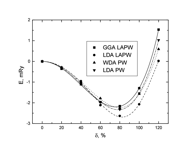
Figure 1: Total energy as a function of ferroelectric displacement in KNbO₃ within the WDA, LDA and GGA using both planewave pseudopotential (LDA and WDA) and LAPW approaches (LDA and GGA). The displacement $\delta$ is in percent of the experimental displacement of Ref. hewat, . Calculations are at the experimental volume, which effectively coincides with the WDA and GGA volumes.

Next we turn to the ferroelectric instability. The present LDA and WDA calculations done with a planewave pseudopotential method, and earlier LAPW calculations both within the LDA and with GGA density functionals are in agreement with the experimental distortion hewat regarding the soft mode eigenvector. However, both LDA and GGA calculations give a soft mode amplitude that is 20% smaller than the existing experimental value, which was determined by powder neutron diffraction. Interestingly, both LDA and GGA calculationss95 ; s97 for BaTiO₃ give a distortion that agrees very closely, (within 5%) with experiment. Fig. 1 shows the result of WDA calculations of this instability for KNbO₃ at the experimental volume, in terms of the reported experimental distortion. As may be noted, there is some scatter between the curves, which represent three different exchange correlation potentials and two different band structure methods. However, all the calculations are in agreement that there is an instability of order 2 mRy/f.u. and that the distortion is only 80% of the reported experimental distortion. In particular, the WDA does not significantly change the distortion relative the the LDA value. Taken together the results strongly suggest an experimental re-examination of the low temperature structure of KNbO₃.

IV Linear Response in the WDA

As mentioned, LDA systematically overestimates the static dielectric constant, $\varepsilon_{\infty}$. Not only is this itself an important characteristic of ferroelectric materials, it also underscores the fact that the dielectric response in general is not accurately reproduced, which could lead to difficulties calculating small energy differences associated with phonons and lattice distortions. The problem has been discussed in terms of the differences between the real one-electron excitation spectrum and the LDA band structure, primarily to underestimation of the band gap. An apparent paradox here is that the exact DFT theory should reproduce the static response functions, but not the excitation spectrum. The solution of this paradox is that the RPA (random phase) dielectric function, which is directly defined by the one-electron spectrum, is enhanced by the so-called exchange-correlation local field corrections. Correspondingly, a small gap and small local field corrections result in the same $\varepsilon_{\infty}$ as a large gap and large corrections. These corrections, in turn, are defined by the second variation of the exchange-correlation energy, $K_{xc}({\bf r,r}^{\prime})=\delta^{2}E_{xc}/\delta n({\bf r})\delta n({\bf r}^{\prime}).$The LDA provides correct $K_{xc}({\bf r,r}^{\prime})$ only in metals and only in the long range limit.

One of the first attempts to correct this was the formulation of ADA, where $n({\bf r}^{\prime})$ in Eq. (1) is substituted by $n({\bf r}),$ so that $E_{xc}^{ADA}=\int n({\bf r})\epsilon_{xc}[\tilde{n}({\bf r)]}d{\bf r.}$ Then $\tilde{n}({\bf r)}$ is defined as $\tilde{n}({\bf r)=}\int w[|{\bf r-r}^{\prime}|,\tilde{n}({\bf r})]n({\bf r}^{\prime}{\bf)}d{\bf r}^{\prime},$ and the universal function $w$ is chosen so that $\delta^{2}E_{xc}^{ADA}/\delta n({\bf r})\delta n({\bf r}^{\prime})$ gives the correct $K_{xc}({\bf r,r}^{\prime})$ for the uniform gas. Contrary to the WDA, the ADA is not self-interaction free in one electron systems, and thus was never as popular as WDA.

From the beginning there was substantial interest in the behavior of WDA in the delocalized limit IEG . Williams and von Barth IEG(WB) suggested that the WDA should give substantial improvement over the LDA in this limit, but till now no systematic study has been reported. If this conjecture is true, the WDA has a great advantage over any other known approximation to the DFT in the sense that it would accurately reproduce two key physical limits. At least some improvement over LDA is to be expected: in the short range $K_{xc}^{WDA}({\bf r,r}^{\prime})$ remains finite, and correspondingly decay with $q\rightarrow\infty$ in reciprocal space. Smaller $K_{xc}$ will result in weaker local field corrections and in an improvement in $\varepsilon_{\infty}$. It is not clear a priori, though, how much $K_{xc}^{WDA}(q)$ is improved over the LDA over the whole $q$ range and, if the improvement is only modest, whether or not an approximation based on the WDA exists that does provide proper behavior. Here we derive an expression for $K_{xc}$ in the WDA, calculate $K_{xc}$ for popular flavors of WDA, and discuss construction of a WDA method with improved $K_{xc}$.

We start by deriving a closed expression for $K_{xc}$ in the WDA for arbitrary $G.$ First some notation: denote the product $(e^{2}/r)G(r)$ as $W(r),$ use atomic units ($e=1,$ $\hbar=1),$ and use primes for the derivative with respect to the density argument, e.g. $G^{\prime}=dG/dn.$ We also introduce two functions, reflecting implicit dependence of the weighted density $\bar{n}$ on variations of the real density:

$$d({\bf r}^{\prime}{\bf-r}) = \delta\bar{n}({\bf r}^{\prime})/\delta n({\bf r})$$ (3)

$$f({\bf r}^{\prime}{\bf-r,r}^{\prime}{\bf-r}^{\prime\prime}) = \frac{\delta^{2}\bar{n}({\bf r}^{\prime})}{\delta n({\bf r})\delta n({\bf r}^{\prime\prime})}=\frac{\delta d({\bf r}^{\prime}{\bf-r})}{\delta n({\bf r}^{\prime\prime})}.$$ (4)

Using the WDA expression for the exchange-correlation energy,

$$E_{xc}=(1/2)\int n({\bf r})n({\bf r}^{\prime})W[|{\bf r-r}^{\prime}|,\bar{n}({\bf r)]}d{\bf r}d{\bf r}^{\prime},$$ (5)

we express $K_{xc}$ in terms of functions $d$ and $f,$ and find these functions using the normalization condition.

$$\int d{\bf r}^{\prime}n({\bf r}^{\prime})G[|{\bf r-r}^{\prime}|,\bar{n}({\bf r})]=-1.$$ (6)

We proceed then in reciprocal space, which corresponds to using density perturbation of the form $\delta n({\bf r)=}n_{q}e^{i{\bf qr}}$. Let $W_{q},$ $G_{q},$ $d_{q}$ and $f_{p,q}$ be the Fourier transforms of the corresponding functions. Then

$$d_{q}=-G_{q}/ng_{0}^{\prime}.$$ (7)

Since at $q\rightarrow 0$ the LDA should be restored,

$$\int d{\bf r}^{\prime}W[|{\bf r-r}^{\prime}|,n]=2\epsilon_{xc}/n.$$ (8)

From this it immediately follows that

$$G_{0}=-1/n,\qquad W_{0}=2\epsilon_{xc}/n.$$ (9)

Thus $d_{q}=-nG_{q}.$ Next variation of Eq.(6) gives us $f_{p,q}.$ In fact, we need only diagonal elements, $f_{q,-q}$, for which we find $f_{q,-q}=2nG_{q}(nG_{q}^{\prime}+G_{q}).$ The second variation of Eq.(5) in terms of $d$ and $f$ is

$$K_{xc}(q)=W_{q}+nd_{q}W_{q}^{\prime}+nd_{q}W_{0}^{\prime}+\frac{n^{2}}{2}(d_{q}^{2}W_{0}^{\prime\prime}+n^{2}f_{q,-q}W_{0}^{\prime}).$$

resulting in

$$K_{xc}(q)=W_{q}-n^{2}G_{q}(W_{q}^{\prime}+W_{0}^{\prime})+n^{2}(n^{2}G_{q}^{2}W_{0}^{\prime})^{\prime}/2.$$ (10)

The original formulation of the WDA used the homogeneous electron gas function for $G$. Since then, three forms of $G$ have been used in calculations, all of which result in improvement over LDA (in the admittedly limited number of tests performed to date). These are: the function $G$ derived for the uniform gas by Perdew and WangPW , the Gunnarsson-Jones function $G^{GJ}(r)=C_{1}(n)\{1-\exp[-\left(\frac{r}{C_{2}(n)}\right)^{-5}]\},$ and the Gritsenko et al. Gri function $G^{GRBA}(r)=C_{1}(n)\exp[-\left(\frac{r}{C_{2}(n)}\right)^{k}]\},$ $k=1.5$ (note that the uniform gas functionPW is approximately given by the same expression with $k=2$). We tested these functions for the densities $r_{s}=1,$ $2,$ and 5 and obtained modest agreement with the Monte Carlo resultsMC (Cf. the left panel of Fig.2, where we plot the calculated exchange-correlation local field factor $I_{xc}(q)=\frac{q^{2}}{4\pi}K_{xc}(q),$ and compare it with Monte Carlo dataMC ). By construction, $K_{xc}(0)$ is correct (and is in fact the LDA value). At $q\approx 1.5-1.8k_{F}$ $K_{xc}$ falls below its LDA value and continues to decrease at large $q$’s. However, a closer look reveals some disagreements: first, $I_{xc}^{WDA}(q)$ is considerably larger than the Monte-Carlo data for the wave vectors between $\approx 0.5k_{F}$ and $1.5k_{F}$. Second, $I_{xc}(q)$ in WDA tends to a constant value, while in Monte Carlo calculations it is $K_{xc}(q)$ itself that has a finite limit at $q\rightarrow\infty,$ and $I_{xc}(q)\rightarrow const\cdot q^{2}$ at $q\rightarrow\infty.$

Figure 2: Left panel: exchange-correlation local field factor in the WDA of Ref. GJ, (Gunnarsson-Jones), Ref.Gri, (Gritsenko et al.), and derived from the homogeneous electron gas pair correlation function (Perdew-Wang), as compared with the Monte Carlo results (Monte Carlo) and the interpolating formula thereof (MC interpolation), as given in Ref. MC, . Densities, from top to bottom, correspond to $r_{s}=1,2,5$. Right panel: the same for the modified WDA of Eq.16. Also the analytical formula of Farid et al. Ref. farid, is shown.

Can one correct these two deficiencies without compromising the correct one-electron limit of WDA? As discussed above, there is no particular reason to use the homogeneous electron gas pair correlation function for $G$ (nor, as discussed above, the exact pair correlation function for the inhomogeneous system, even if it had been known). Since using $G_{0}$ in WDA does not guarantee any improvement in describing properties of the homogeneous gas itself, one may use the freedom in $G(r)$ to adjust the WDA so that the calculated local field factor (and thus linear response function) is as accurate as possible. Inversion of eq.(10) yields $G(q)$ for a given $K_{xc}(q).$ It does not guarantee, however, that the result will be physical. So, as a first step, let us analyze Eq. (10). Let us first mention that the real $K_{xc}(q)$ changes its behavior from the long range limit to the short range limit near $q=2k_{F},$ which plays the role of the inverse length scale. What is the characteristic length scale in WDA? To find that, we write $G_{q}=-\varphi(p/Q)/n$, with the condition $\varphi(0)=1,$ where $Q$ is some constant (both the Gunnarsson-Jones and the Gritsenko et al. functions are of this form). Then

$$W_{0}=\frac{2}{\pi}\int_{0}^{\infty}G_{q}dq=-\frac{2Q}{\pi n_{0}}\int_{0}^{\infty}\varphi(x)dx=\frac{2\epsilon_{xc}(n_{0})}{n_{0}}.$$ (11)

If we now define $Q(n)=-\pi\epsilon_{xc}(n),$ then the second condition on $\varphi(x)$ becomes $\int_{0}^{\infty}\varphi(x)dx=1.$ These two conditions reduce our freedom to adjust $G_{q}:$ since the characteristic size of $\varphi(x)$ is of order of 1, the wave vector dependence of $G_{q}$ is defined by the ratio $q/Q=-q/\pi\epsilon_{xc}.$ Apparantely, varying the shape of the function $\varphi$ will not significatntly change the lentgh scale of the resulting $K_{xc}(q).$ Explicitly density-dependent functions $\varphi(x,n)$ may be needed to shift the hump from its position of $q\approx 1.5k_{F}$ to $q\approx 2k_{F}.$ It is still an open question whether or not a physically sound function can be found with this property.

However, even if the “$2k_{F}$” problem is fixed, another, probably even more important problem remains: the short wave length behavior of $K_{xc}.$ It is easy to see that if $G(q)\rightarrow 0$ at $q\rightarrow\infty,$ then $W_{p}\rightarrow const/p^{2}$ at $p\rightarrow\infty,$ and so does, according to Eq.(10), $K_{xc}.$ On the other hand, as mentioned above, the correct $K_{xc}(q)$ goes to a constant at $q\rightarrow\infty$ as $q^{2},$ although the constant is smaller than $K_{xc}^{LDA}$. This result was predicted by Holas Holas and is physically important: it comes from the exchange-correlation contribution to kinetic energy (which is essentially local and decays slower with $q$ than the interaction part of $E_{xc}).$ The present WDA misses the corresponding physics. Fortunately, this is easy to correct. Farid et al.farid tabulated the coefficient $\gamma$ that defines the asymptotic behavior of $K_{xc}(q\rightarrow\infty)$ as $K_{xc}(q\rightarrow\infty)=-\frac{4\pi}{q^{2}}\gamma(n)\frac{q^{2}}{k_{F}^{2}},$ where $\gamma(n)$ is a universal function, parametrized in Ref.farid . Let us now modify the function $G(r)$

$$G(r)=G_{1}(r)+G_{2}(r)=A\delta(r)/4\pi r+G_{2}(r),$$ (12)

Since $\int G_{1}(r)r^{2}dr=0,$ the normalization condition for $G_{2}$ is the same as for $G$ itself. Since $4\pi\int G_{1}(r)rdr=A,$ the LDA limit condition for $G_{2}$ becomes

$$4\pi\int G_{2}(r)rdr = 2\tilde{\epsilon}_{xc}(n)/n,$$

$$\tilde{\epsilon}_{xc}(n) = \epsilon_{xc}(n)-An/2.$$ (13)

Thus

$$A = -4\pi\gamma(n)/k_{F}^{2},$$

$$\tilde{\epsilon}_{xc}(n) = \epsilon_{xc}(n)+2\pi n\gamma(n)/k_{F}^{2}$$ (14)

Now $G_{p}=G_{2p},$ $W_{p}=A+W_{2p},$ and $W_{p}^{\prime}=A^{\prime}+W_{2p}^{\prime},$

$$K_{xc}(q) = A+W_{2q}-n^{2}G_{2q}(A^{\prime}+W_{2q}^{\prime}+W_{2,0}^{\prime})+n^{2}(n^{2}G_{q}^{2}W_{2,0}^{\prime})^{\prime}$$ (15)

$$= A-n_{0}^{2}G_{2p}A^{\prime}+\tilde{K}_{xc},$$

where $\tilde{K}_{xc}$ is calculated from $\tilde{\epsilon}_{xc}$ in exactly the same way as $K_{xc}$ is calculated from $\epsilon_{xc}.$ The corresponding functional for the exchange-correlation energy is

$$E_{xc}^{AWDA}=\frac{1}{2}\int\frac{n({\bf r})n({\bf r}^{\prime})}{(|{\bf r-r}^{\prime}|)}G[|{\bf r-r}^{\prime}|,\bar{n}({\bf r)]}d{\bf r}d{\bf r}^{\prime}+\int n({\bf r})\tilde{\epsilon}_{xc}[n({\bf r})]d{\bf r}.$$ (16)

Here $G(r)$ is normalized to $\tilde{\epsilon}_{xc}(\bar{n})$ instead of $\epsilon_{xc}(\bar{n}).$ In practice, the first term gives rise to the standard expression for the WDA potentialGJL ; AG , and the second yields two additional terms, one from the variation of $n({\bf r})$, and the other arising from $\delta\bar{n}({\bf r^{\prime})}/\delta{n}({\bf r)}$. Since we do not require that $G(r)=\int_{0}^{1}[g(r;\lambda,\bar{n})-1]d\lambda.,$ where $g$ corresponds to the uniform gas, but rather consider it to be a flexible function satisfying two normalization conditions, further improvement of the method should be possible along the line described in the previous paragraph, namely the freedom in choosing $G(r)$ can be used to yield $K_{xc}$ according to Eq. (15) close to the linear response of the homogeneous electron gas, including correct behavior near $q=2k_{F}$. In the right panel of Fig. 2, we show $I_{xc}$ calculated according to Eq. 16 with the different functional form of $G(r).$ Clearly, the results are much better than either the LDA or “conventional” WDA.

In short, we have calculated the exchange-correlation local field function $K_{xc}$ in the WDA, and found that besides the expected improvement over the LDA it has two major deficiencies: (1) it does not have correct asymptotic behavior at $q\rightarrow\infty,$ and (2) the characteristic feature at $q\approx 2k_{F}$ is displaced towards smaller $q$’s. The former can be easily corrected by adding a delta-function component to $G(r),$ which results in Eq. (16). The latter is harder to fix, but there are still unused degrees of freedom in the formalism which may be used to tune the behavior near $2k_{F}.$ Intuitively (cf. Ref.IEG(WB) ), a method which retains exact one-electron limit of WDA, and at the same time is accurate in the opposite limit of the nearly uniform electron gas, seems promising for practical applications. However, tests on real materials will be needed to determine whether or not this modification of the WDA is advantageous in practice.

V Conclusions

WDA calculations of the equilibrium volume of several oxides show that with the electron gas form of $G$ and shell partitioning, the WDA yields much improved volumes over the LDA and GGA. No case was found where the WDA degrades the LDA results. Phonon frequencies and the ferroelectric distortion in KNbO₃ are in good accord with LDA predictions provided that the LDA calculations are performed at the experimental volume, which is effectively the same as the WDA volume. The direction of the ferroelectric soft mode is in good agreement with experiment, but all exchange correlation functionals tested yield a distortion that is 20% smaller than that reported in the powder neutron experiment of Hewat.hewat The implication is that this displacement should be re-examined from an experimentally. The above results combined with the fact that the WDA linear response of the electron gas is in substantially better agreement with Monte Carlo data than the LDA, and that, if desired, the approach has the flexibility to further improve this property, is suggestive that the WDA may be a generally more reliable method than the LDA.

We are thankful for helpful discussions with L.L. Boyer, H. Krakauer, O. Gunnarsson and R. Resta. This work is supported by the Office of Naval Research. Calculations were performed using DoD HPCMO facilities at NAVO and ASC. The CHSSI DoD Planewave code was employed for some of the calculations.

References

- (1) See for example, Proceedings of The Fourth Williamsburg Workshop on First Principles Calculations for Ferroelectrics, R.E. Cohen, ed., Ferroelectrics 194, 1 (1997).
- (2) R.E. Cohen, Nature (London) 358, 136 (1992).
- (3) R.E. Cohen and H. Krakauer, Ferroelectrics 136, 65 (1992).
- (4) D.J. Singh and L.L. Boyer, Ferroelectrics 136, 95 (1992).
- (5) A.V. Postnikov, T. Neumann, G. Borstel and M. Methfessel, Phys. Rev. B 48, 5910 (1993)
- (6) A.V. Postnikov, T. Neumann and G. Borstel, Ferroelectrics 164, 101 (1995).
- (7) R. Yu and H. Krakauer, Phys. Rev. Lett. 74, 4067 (1995).
- (8) C.-Z. Wang, R. Yu and H. Krakauer, Ferroelectrics 194, 97 (1997).
- (9) D.J. Singh, Ferroelectrics 164, 143 (1995).
- (10) D.J. Singh, Ferroelectrics 194, 299 (1997).
- (11) R.E. Cohen and H. Krakauer, Phys. Rev. B 42, 6416 (1990).
- (12) D.J. Singh, Phys. Rev. B 52, 12559 (1995).
- (13) S. Teslic, T. Egami and D. Viehland, Ferroelectrics 194, 271 (1997).
- (14) H. Fujishita and S. Katano, J. Phys. Soc. Jpn. 66, 3484 (1997).
- (15) A. Dal Corso, S. Baroni and R. Resta, Phys. Rev. B 49, 5323 (1994).
- (16) R. Resta, Ferroelectrics 194, 1 (1997).
- (17) S. DallOlio, R. Dovesi and R. Resta, Phys. Rev. B 56, 10105 (1997).
- (18) G. Saghi-Szabo, R.E. Cohen and H. Krakauer, unpublished.
- (19) O. Gunnarsson, M. Jonson, and B.I. Lundquist, Phys. Lett. 59A, 177 (1976).
- (20) O. Gunnarsson, M. Jonson, and B.I. Lundquist, Solid State Commun. 24, 765 (1977).
- (21) J.A. Alonso and L.A. Girifalco, Phys. Rev. B, 17, 3735 (1978).
- (22) O. Gunnarsson, M. Jonson, and B.I. Lundquist, Phys. Rev. B, 20, 3136 (1979).
- (23) D.J. Singh, Phys. Rev. B, 48, 14099 (1993)
- (24) M. Sadd and M.P. Teter, Phys. Rev. B, 54 13643 (1996).
- (25) J.P.A. Charlesworth, Phys. Rev. B, 53, 12666 (1996).
- (26) Ref.char, is an exception, but note that the LDA results of this work differ from most previous calculations.
- (27) Theory of the inhomogeneous electron gas, Ed. by S. Lundqvist and N.H. March (Plenum, New York, 1983).
- (28) J.P. Perdew and Y. Wang, Phys. Rev. B 46, 12947 (1993).
- (29) See for example, S. Goedecker and C.J. Umrigar, Phys. Rev. A 55, 1765 (1997), and references therein.
- (30) O. Gunnarsson and R.O. Jones, Physica Scripta, 21, 394 (1980).
-
(31)
D.J. Singh, S.A. Kajihara, S.G. Kim, C. Woodward, DoD Planewave:
A General
Scalable Density Functional Code, cst-www.nrl.navy.mil/people/singh/planewave. - (32) D.J. Singh, H. Krakauer, C. Haas and A.Y. Liu, Phys. Rev. B 46, 13065 (1992).
- (33) N. Troullier and J.L. Martins, Phys. Rev. B 43, 1993 (1991).
- (34) D.J. Singh Planewaves Pseudopotentials and the LAPW Method (Kluwer, Boston, 1994).
- (35) W. Zhong, R.D. King-Smith and D. Vanderbilt, Phys. Rev. Lett. 72, 3618 (1994).
- (36) M.D. Fontana, G. Metrat, J.L. Servoin and F. Gervais, J. Phys. C 17, 483 (1984).
- (37) A.W. Hewat, J. Phys. C 6, 2559 (1973).
- (38) A.R. Williams and U. von Barth, in Ref. IEG, .
- (39) O.V. Gritsenko, A. Rubio, L.C. Balbás, and J.A. Alonso, Chem. Phys. Lett 205, 348 (1993)
- (40) S. Moroni, D.M. Ceperley, and G. Senatore, Phys. Rev. Lett 75, 689 (1995).
- (41) A. Holas, in Strongly Coupled Plasma Physics, ed. by F.J. Rogers and H.E. De Witt (Plenum, NY, 1987)
- (42) B. Farid, V. Heine, G.E. Engel, and I.J. Robertson, Phys. Rev. B 48, 11 602 (1993).