Phase separation in the 2D Hubbard model:
a fixed-node quantum Monte Carlo study

Abstract

Fixed-node Green’s function Monte Carlo calculations have been performed for very large $16\!\times\!16$ 2D Hubbard lattices, large interaction strengths $U\!=\!10,20,$ and $40$, and many ($15\sim 20$) densities between empty and half filling. The nodes were fixed by a simple Slater-Gutzwiller trial wavefunction. For each value of $U$ we obtained a sequence of ground-state energies which is consistent with the possibility of a phase separation close to half-filling, with a hole density in the hole-rich phase which is a decreasing function of $U$. The energies suffer, however, from a fixed-node bias: more accurate nodes are needed to confirm this picture. Our extensive numerical results and their test against size, shell, shape and boundary condition effects also suggest that phase separation is quite a delicate issue, on which simulations based on smaller lattices than considered here are unlikely to give reliable predictions.

Strongly correlated electrons and holes are expected to play a key role in the high-$T_{c}$ superconductors. Their possible instability towards phase separation (PS), initially believed to inhibit superconductivity, is attracting a lot of interest since a few different authors [1, 2, 3] have pointed out that such a tendency may in fact be intimately related to the high-$T_{c}$ superconductivity. Long-range repulsive interactions may turn the PS instability into an incommensurate charge-density-wave (ICDW) instability, and the very existence of a quantum critical point associated to it may be a crucial ingredient of the superconducting transition [4]. PS and/or ICDW instabilities are related to a substantial reduction of the kinetic energy, which otherwise tends to stabilize uniformly distributed states; such a reduction is typical of strongly correlated electrons, both in real and model systems.

PS has been experimentally observed in La₂CuO_4+δ[5, 6], where the oxygen ions can move: in the doping interval $0.01\leq\delta\leq 0.06$ the compound separates into a nearly stoichiometric antiferromagnetic phase and a superconducting oxygen-rich phase. In generic compounds, where charged ions cannot move, the possibility of a macroscopic PS is spoiled by the long-range Coulomb repulsion, and should lead to an incommensurate CDW instability [7]; here the identification of charge inhomogeneities with spoiled PS is less straightforward [8]. On the theoretical side, evidence for PS has been suggested for various models of strongly correlated electrons, as the $t\!-\!J$ model [9], the three-band Hubbard model, the Hubbard-Holstein model and the Kondo model (see e.g. Ref. [4] and references therein).

Despite intensive studies, even for simple models there is no general agreement on the PS boundary: for the very popular $t\!-\!J$ model, PS is fully established only at large $J$, but at small $J$ (which unfortunately happens to be the physically relevant case) theoretical and numerical results are quite controversial. Emery et al.’s [9] theory that PS occurs at any value of $J$ in the $t\!-\!J$ model is confirmed by a recent numerical study by Hellberg and Manousakis [10], but is in contrast with Dagotto et al.’s [3] exact numerical results on small clusters, suggesting no tendency toward PS for both the Hubbard model and the $t\!-\!J$ model below a critical value $J<J_{c}\sim t$, and with Shih et al.’s [11] numerical results. We also mention the recent suggestion by Gang Su [12], according to which the Hubbard model does not show PS at any value of $U/t$ for any finite temperature, although it does not apply to ground-state properties.

PS is a thermodinamic instability associated to the violation, in a given density range $n_{1}<n<n_{2}$, of the stability condition $\chi^{-1}={\partial}^{2}\!{\cal E}/\partial{n^{2}}>0$, which requires the energy density ${\cal E}$ of an infinite electronic system to be a convex function of the electron density $n$. The system will therefore separate into two subsystems with electron densities $n_{1}$ and $n_{2}$. For the two-dimensional $t$-$J$ and Hubbard models, PS, if any, is expected to occur in a density range close to half filling ($n\simeq 1$), and to yield a hole-rich phase with density $n_{1}<1$ and a hole-free phase with density $n_{2}=1$ [9]. In a truly infinite system such a PS would be associated with a vanishing inverse compressiblity $\chi^{-1}$ in the whole density range $n_{1}<n<n_{2}$; in a finite system $\chi^{-1}$ may even become negative, because of surface effects. So for finite systems it’s preferable to pinpoint the PS using a Maxwell’s construction (originally suggested by Emery, Kivelson and Lin [9], see also below). But even such a procedure can give reliable results only for medium-large finite systems; really small systems (for which most numerical results have been up to now available) can attain so few and coarse densities, and suffer from so large finite-size errors, that their predictions on the relevant trends remains largely inconclusive.

Under these circumstances the availability of the fixed-node Green’s function Monte Carlo (FNMC), a new and powerful numerical technique [13] which allows the study of (previously unfeasible) large lattice-fermion systems, provides us with a powerful tool to further investigate the Hubbard model. Whether the $2D$ Hubbard hamiltonian, a prototype for interacting electrons with no long-range repulsion, shows any instability towards PS, is a very interesting open question. A numerical study may also shed some indirect light on two related issues: the $t\!-\!J$ model in the physical region of small $J$, and the adequacy of the one-band Hubbard hamiltonian to catch an essential aspect of high-$T_{c}$ superconductors.

To evaluate the ground-state energy of the Hubbard hamiltonian

$$H=-t\sum_{\langle i,j\rangle\sigma}(c^{\dagger}_{i\sigma}c_{j\sigma}+h.c.)+U\sum_{i}n_{i\uparrow}n_{i\downarrow}$$ (1)

we thus implemented the FNMC method recently proposed for lattice fermions by van Bemmel et al. [13, 14], which has been used by Boninsegni for frustrated Heisenberg systems [15] and by Gunnarsson et al. for orbitally-degenerate Hubbard models [16].

The Green’s function Monte Carlo, after a sufficiently long imaginary time, projects out the ground-state component of any initial wavefunction; apart from transient estimates, which for large systems appear to be hazardous unless the initial variational wavefunction is sufficiently close to the exact one, this method is therefore not directly usable for fermions in our Hubbard model (as well as any other model whose Green’s function is not positive everywhere). The FNMC [13, 14] replaces the true hamiltonian by an effective hamiltonian which confines the Monte Carlo random walk within a single nodal region (a region of the configuration space where the guiding wavefunction never changes sign), and, in analogy with the continuum case [17, 18], it provides an upper bound for the true ground-state energy [14].

We also implemented the tecnique proposed in Ref.[19], which allows us to reproduce with a relatively small fixed number ($100\sim 200$) of walkers equally accurate results as those obtained by means of standard MC runs of more than $2000$ walkers.

The variational wavefunctions we use to guide the random walks and to fix the nodes are the product of a Gutzwiller factor and two Slater determinants of single-particle, mean-field wavefunctions for up- and down-spin electrons. The optimal Gutzwiller parameter and mean-field wavefunctions (whose only parameter is the staggered magnetization) were preliminarly obtained, for each $U$ and density, by variational Monte Carlo (VMC) runs.

A few representative variational and FNMC energies are shown in Table I for the $4\!\times\!4$ Hubbbard lattice, for which exact results [20] are available. As expected, the VMC energy is always above the FNMC energy, which for these coupling strengths is slightly ($\sim 3\%$) above the exact energy. For comparison we show the Constrained-Path Monte Carlo (CPMC) energies of Zhang et al. [21], which also include a larger $16\!\times\!16$ lattice (last row). Especially at large $U$’s our results appear of comparable quality as theirs. As far as the $4\!\times\!4$ results are concerned, we notice that for $N_{e}=10$, which corresponds to a closed-shell configuration, both FNMC and CPMC are much closer to the exact energy than for $N_{e}=14$, which corresponds to an open-shell configuration. This could be a serious problem when numerically studying the behavior of the energy as a function of the density; the results presented here fortunately show that, for lattices larger than $12\!\times\!12$, the shell effects become almost irrelevant.

To study the energy as a function of the electron density we have first tried out the less usual way of varying the density suggested by Ref. [10] to avoid spurious Fermi-surface shape effects (keep the number of electrons $N_{e}$ fixed while the size of the underlying lattice is being varied), but discovered that either the number of electrons is really small (e.g. $N_{e}\!=\!16$), and then artificial changes in the convexity of the curve may occur, or the system is large enough (e.g. $12\!\times\!12$ lattices or larger), and then it doesn’t matter how the density is being varied. So for our systematic study (many densities and three $U$ values) we stick to a large $16\!\times\!16$ lattice ($N_{s}\!=\!256$ sites), and vary the number of electrons $N_{e}$ to yield electronic densities $n\!=\!N_{e}/N_{s}$ ranging from empty $n\!=\!0$ to half filling $n\!=\!1$. In the first panel of Fig. 1 we show the electronic ground-state energy per site, obtained by FNMC runs as a function of the density[22]. Energies are in units of the hopping parameter $t$ throughout this paper; the statistical errors are smaller than the marker size, and thus are not visible here. The calculated points are shown as full markers for closed shells, and as empty markers for open shells. From Fig. 1 (see caption) it appears that the open-shell error, significant for a small $4\!\times\!4$ lattice (see Table I), becomes of the order of the statistical error (and thus negligible) for our large lattices [23].

At all densities our three sets of data for $U\!=\!10$ (lower), $20$ (middle), and $40$ (upper curve) are bracketed by the noninteracting unpolarized energy and the fully spin-polarized energy (both dashed in Fig. 1), and display a smooth and reasonable behavior. To evaluate the absolute accuracy of our results, we can rely on two exact limits: the low-density ($n\!\simeq\!0$) regime, where we expect ${\cal E}=-4n$, and the half filled case ($n\!=\!1$),for which the strong-coupling expansion provides the correct large $U$ behavior: to leading order in $t/U$, the model maps onto an Heisenberg model, whose ground-state energy has been evaluated with great accuracy [19, 24]. We can also consider the next correction term $34.6t^{4}/U^{3}$ [25]. At low density our results are essentially exact; at half filling our error is small ($\sim\!3\%$) for $U=10$ but (as already seen in Table I) it tends to grow with $U$: $\sim\!9\%$ for $U=20$ and $\sim\!11\%$ for $U\!=\!40$. We have made sure (see markers other than dots in Fig. 1 and footnote [22]) that such an energy discrepancy is not due to finite-size, shape, open-shell, and boundary condition effects; as far as systematic errors are concerned, we are thus left with the fixed-node approximation: as $U$ grows, more flexible trial wavefunctions than adopted here are required to obtain accurate nodes [26].

Keeping in mind the virtues and limitations of our numerical study, we can now turn to PS in the Hubbard model. It has been shown in Ref.[9] that the Maxwell construction is equivalent to study, as a function of the hole density $x\!=\!1\!-\!n$, the quantity $e(x)\!=\![e_{h}(x)\!-\!e_{H}]/x$, i.e. the energy per hole $e_{h}(x)$ measured relative to its value at half filling $e_{H}=e_{h}(x\!=\!0)$. For an infinite system, if the inverse compressibility $\chi^{-1}$ vanishes between some critical density $n_{c}<1$ and half filling $n=1$, then for $0\leq x\leq x_{c}$ the function $e(x)$ is a constant, and the fingerprint of a PS is thus a horizontal plot of $e(x)$ below $x_{c}$. For a finite system, instead, the PS fingerprint is a minimum of $e(x)$ at $x=x_{c}$ [9]. In some sense, $e(x)$ works like a magnifying lens of PS. It should be stressed that in a consistent definition of $e(x)$ the half-filling energy $e_{H}$ must be obtained as $e_{h}(x\!=\!0)$ from the same calculation as any other $e_{h}(x\neq 0)$ (in this work, from our FNMC). If that’s not the case, then $e(x)$ may tend to diverge near $x\!=\!0$, with the danger of artificially creating, rather than magnifying, the occurrence of PS. In the three right panels of Fig. 1 we find plots of $e(x)$ for $U=10$, $20$, and $40$; these values, as well as the associated error bars, are obtained from those of the first panel (original FNMC energies and tiny error bars). Despite the error bars, a common trend is evident for all the calculated coupling strenghts: $e(x)$ has a positive slope for large hole densities, far from half-filling, but then it clearly changes slope below some small critical density $x_{c}$. Such a minimum in $e(x)$ implies that, at least for the FNMC effective hamiltonian determined by our choice of wavefunction, PS occurs below $x=x_{c}$ [27]. Although a finer grid of hole densities would be required to locate with high precision the critical density $x_{c}$ as a function of $U$, we already see that $x_{c}$ decreases as $U$ is increased; this qualitatively agrees with the original predictions [9] and with some previous calculations on the $t\!-\!J$ model at corresponding values of $J=4t^{2}/U$ [10].

In summary, our extensive FNMC numerical simulations of the Hubbard model for $16\!\times\!16$ two-dimensional lattices suggest PS for $U\gg t$. If confirmed by further fixed-node simulations based on different nodes [26] (and possibly even larger lattices [27]), this result would imply that the $t\!-\!J$ model is also likely to show PS in the physically relevant regime $\!J<\!0.4$, and that even a single-band Hubbard model is sufficient to reproduce this physical tendency of high-$T_{c}$ superconductors.

We thank M. Boninsegni, S. Sorella, O. Gunnarsson, F. Becca, C. Lavalle, M. Grilli and C. Castellani for useful suggestions and discussions, and A. Filippetti for his precious help. Special thanks are due to V.J. Emery and S.A. Kivelson, whose remarks were of key importance for the final discussion of our results, and to M. Calandra Bonaura and S. Sorella for making available to us the method of Ref. [19] prior to publication and for many kind explanations. GBB gratefully acknowledges partial support from the Italian National Research Council (CNR, Comitato Scienza e Tecnologia dell’Informazione, grants no. 96.02045.CT12 and 97.05081.CT12), the Italian Ministry for University, Research and Technology (MURST grant no. 9702265437) and INFM Commissione Calcolo.

	${\rm size}$	$N_{e}$	$n$	$U$	${\rm VMC}$	${\rm FNMC}$	${\rm CPMC}$	${\rm EXACT}$
	$4\!\times\!4$	$10$	$0.625$	$4$	$-1.211(2)$	$-1.220(2)$	$-1.2238(6)$	$-1.2238$
	$4\!\times\!4$	$10$	$0.625$	$8$	$-1.066(2)$	$-1.086(2)$	$-1.0925(7)$	$-1.0944$
	$4\!\times\!4$	$14$	$0.875$	$8$	$-0.681(2)$	$-0.720(2)$	$-0.728(3)$	$-0.742$
	$4\!\times\!4$	$14$	$0.875$	$12$	$-0.546(2)$	$-0.603(2)$	$-0.606(5)$	$-0.628$
	$16\!\times\!16$	$202$	$0.789$	$4$	$-1.096(2)$	$-1.107(5)$	$-1.1193(3)$	$-$

TABLE I.: Ground-state energy per site (in units of the hopping parameter $t$) for a $4\!\times\!4$ Hubbard lattice and various values of $U$. $N_{e}$ is the number of electrons and $n$ is the corresponding average density. VMC: variational Monte Carlo, this work; FNMC: Fixed-Node Green’s function Monte Carlo, this work; CPMC: Constrained-Path Monte Carlo, Ref. [21]; EXACT: exact diagonalization results, Ref. [20].(see text)

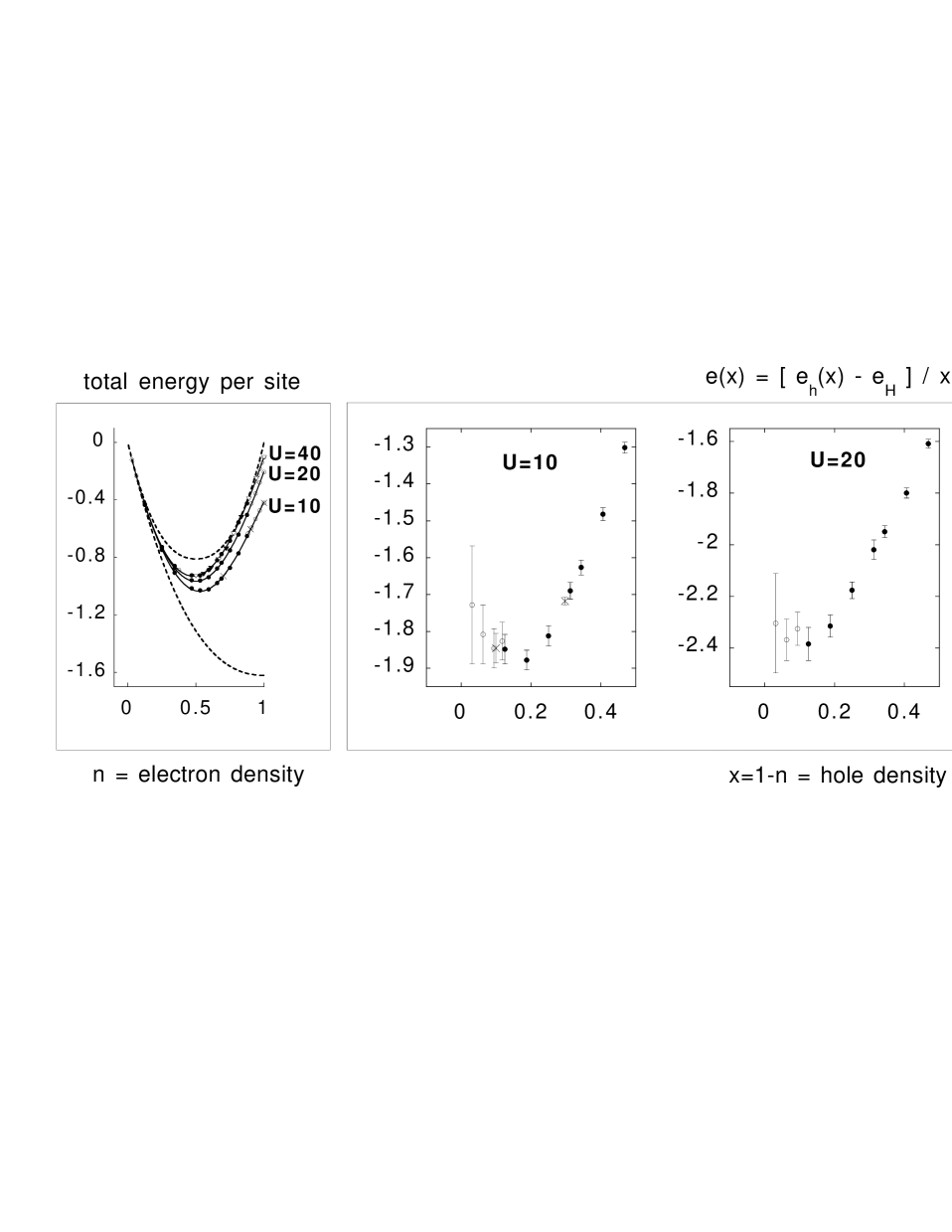
FIG. 1.: The first panel, to the very left, shows the ground-state energy per site (in units of the hopping parameter $t$) as a function of the electronic density, for a 2D Hubbard lattice of $N_{s}=16\!\times\!16=256$ sites with $U=10$ (lower), $20$ (middle), and $40$ (upper data). Errors are smaller than the marker size. Full markers correspond to closed shells and empty markers correspond to open shells. The dashed curves correspond to two (analytically given) $U=0$ results: the fully spin-polarized case (upper curve), whose total energy per site is symmetric with respect to quarter filling, and the unpolarized case (lower curve), whose total energy per site is symmetric with respect to half filling. Triangles (corresponding to a smaller $12\!\times\!12$ lattice and $U=40$) and crosses ($11\sqrt{2}\times 11\sqrt{2}$ lattice and $U=10$) are shown for comparison (see text). The second, third and fourth panel to the right contain plots of $e(x)$ vs. $x$ (see text) for $U=10$, $20$, and $40$, respectively. The data markers have the same meaning as in the first panel; obviously at small $x$ the error bar associated to $e(x)$, $\Delta{e(x)}=[\Delta{e}_{h}(x)+\Delta{e}_{h}(x\!=\!0)]/x$, becomes significant even if the statistical FNMC error $\Delta{e}_{h}(x)$ is tiny (see text).

REFERENCES

- [1] M. Grilli, R. Raimondi, C. Castellani, C. Di Castro, and G. Kotliar, Phys. Rev. Lett. 67, 259 (1991); C. Di Castro and M. Grilli Physica Scripta T 45, 81 (1992), and reference therein.
- [2] V.J. Emery, and S.A. Kivelson, Physica C 209, 597 (1993).
- [3] E. Dagotto, A. Moreo, F. Ortolani, D. Poilblanc and J. Riera, Phys. Rev. B 45, 10741 (1992).
- [4] C. Castellani, C. Di Castro, M. Grilli, Phys. Rev. Lett. 75, 4560 (1995).
- [5] J.D. Jorgensen, B. Dabrowski, Shiyon Pei, D.G. Hinks, L. Soderholm, B. Morosin, J.E. Schirber, E.L. Venturini, and D.S. Ginley, Phys. Rev. B 38, 11337 (1988).
- [6] F.C. Chou et al., Phys. Rev. B 54, 572 (1996).
- [7] J.M. Tranquada, B.J. Sternleb, J.D. Axe, Y. Nakamura, and S. Uchida, Nature 375, 561 (1995).
- [8] A. Bianconi, N.L. Saini, A. Lanzara, M. Missori, T. Rossetti, H. Oyanagi, H. Yamaguchi, K. Oka, and T. Ito, Phys. Rev. Lett. 76, 3412 (1996).
- [9] V.J. Emery, S.A. Kivelson, H.Q. Lin, Phys. Rev. Lett. 64, 475 (1990).
- [10] C.S. Hellberg and E. Manousakis, Phys. Rev. Lett. 78, 4609 (1997).
- [11] C.T. Shih, Y.C. Chen and T.K. Lee, Phys. Rev. B 57, 627 (1998).
- [12] Gang Su, Phys. Rev. B 54, R8281 (1996).
- [13] H.J.M. van Bemmel, D.F.B. ten Haaf, W. van Saarloos, J.M.J. van Leeuwen, G. An, Phys. Rev. Lett. 72, 1442 (1994).
- [14] D.F.B. ten Haaf, H.J.M. van Bemmel, J.M.J. van Leeuwen, W. van Saarloos, and D.M. Ceperley , Phys. Rev. B 51, 13039 (1995).
- [15] M. Boninsegni, Phys. Rev. B 52, 15304 (1995); Phys. Lett. A 216, 313 (1996).
- [16] O. Gunnarsson, E. Koch, and R.M. Martin, Phys. Rev. B 54, R11026 (1996); ibid. 56, 1146 (1997); F. Aryasetiawan, O. Gunnarsson, E. Koch, and R.M. Martin, Phys. Rev. B 55, 10165 (1997).
- [17] J.B. Anderson, J. Chem. Phys. 63, 1499 (1975).
- [18] D.M. Ceperley, Physica B 108, 875 (1981).
- [19] M. Calandra Bonaura and S. Sorella, Phys. Rev. B 57, 11446 (1998).
- [20] A. Parola, S. Sorella, S. Baroni, R. Car, M. Parrinello, and E. Tosatti, Physica C 162-164, 771 (1989); A. Parola, S. Sorella, M. Parrinello, and E. Tosatti, Phys. Rev. B 43, 6190 (1991).
- [21] Shiwei Zhang, J. Carlson, and J.E. Gubernatis, Phys. Rev. Lett. 74, 3652 (1995).
- [22] Different boundary conditions yield energies within an error bar for lattices and within at most two error bars for our smallest lattices; all results presented here refer to antiperiodic boundary conditions.
- [23] We have checked a few densities which correspond to open shells in our usual lattice (empty dots in the first panel of Fig. 1), but to closed shells in a -rotated lattice (crosses in the first panel of Fig. 1); the energy difference turns out to be negligible.
- [24] Q.F. Zhong and S. Sorella, Europhys. Lett. 21, 629 (1993).
- [25] This term has been proposed long ago by Takahashi, J. Phys. C 10, 1289 (1977); the resulting large- expansion agrees remarkably well, for , with the more recent results of G. Polatsek and K.W. Becker, Phys. Rev. B 54, 1637 (1996).
- [26] The Gutzwiller-Slater wavefunction, a very popular choice for the Hubbard model, suffers from at least two drawbacks (which probably reflect into the “quality” of its nodes): it does not describe a spin singlet and it only has on-site correlations; we are presently trying out more general forms, such as those proposed by T. Giamarchi and C. Lhuillier, Phys. Rev. B 42, 10641 (1990).
- [27] In a finite lattice even for the energy of a tight-binding system would show an artificial phase separation at , due to the high degeneracy at the Fermi level: see H.Q. Lin, Phys. Rev. B 44, 7151 (1991).